Finance Department
How the U.S. Capital Markets Volatility Interacts with
Economic Growth
João Marques
Dissertation submitted as partial requirement for the Master’s degree in Finance
Supervisor:
Prof. Doutor José Dias Curto Quantitative Methods Department
Aos meus queridos pai e mãe pelo apoio ao longo de toda a vida. Á minha familia Cristina e Marta.
I would like to thank my supervisor Professor José Dias Curto, from ISCTE Lisbon University Institute, for all the inspiration and guidance in the thesis.
ABSTRACT
Empirical finance suggests that capital markets volatility has a negative relationship with economic growth, in the United States. However, the main focus has been on the equity market volatility dynamics and less on other equally important asset classes, given their significant role in the structure of capital markets. In this thesis, I examine the leading and lagging dynamics between money markets, government debt, corporate debt and equities volatilities, in the U.S., and a real GDP growth proxy, between January, 1963 and March, 2009. I also introduce the concept of aggregate capital markets portfolio volatility, which follows the assumptions of a mean-variance portfolio calculation, and test its interaction with growth. Moreover, it is analysed the degree of explaining power of volatilities to the GDP proxy in specific time periods and also in NBER recessions, slowdowns and expansions periods. The empirical results posit that asset classes and capital markets portfolio volatilities are essentially counter-cyclical of growth, on a contemporaneous basis. However, this interaction changes significantly across decades. Finally, in recessions and slowdown periods rising volatility leads the economic cycle, but in expansions its downtrend lags the cycle.
Key words: Regression; Capital Markets Portfolio; Equity; Money Markets; Government Debt; Corporate and Financial Debt.
RESUMO
Os estudos empíricos financeiros sugerem que a volatilidade dos mercados de capitais evidencia uma relação negativa com o crescimento económico, nos Estados Unidos. No entanto, o maior foco tem sido sobre a dinâmica da volatilidade do mercado de acções e menos noutras classes de activos, igualmente importantes, dada a sua relevância na estrutura do mercado de capitais. Nesta tese, examino as dinâmicas entre as volatilidades dos mercados monetários, das obrigações do tesouro, das obrigações de risco de crédito e das acções, nos E.U.A., e uma variável próxima do produto interno bruto real, entre Janeiro de 1963 e Março de 2009. Também introduzo o conceito de volatilidade de carteira agregada de mercados de capitais, que obedece aos pressupostos de cálculo de rendibilidade e risco de uma carteira de activos financeiros, e testo a respectiva interacção com o crescimento. Adicionalmente, é analisado o grau de poder explicativo de volatilidades para a variável próxima de crescimento, em periodos de tempo específicos e também em recessões decretadas pelo instituto NBER, em conjunturas de abrandamento e de expansão. Os resultados empíricos sugerem que as volatilidades das classes de activos e da carteira de mercados de capitais são essencialmente contra-cíclicas do crescimento, numa base contemporânea. No entanto, a intensidade desta relação varida de forma substancial entre as várias décadas. Finalmente, em periodos de recessão ou de abrandamento, uma tendência de subida da volatilidade lidera a evolução do cíclo económico, mas em periodos de expansão a respectiva tendência de descida segue o crescimento económico.
Palavras-chave: Regressão; Carteira de Mercados de Capitais; Acções; Mercados Monetários; Dívida Pública; Dívida de Empresas Não Financeiras e Financeiras.
INDEX
1 Introduction 1
2 Theoretical Background 4
2.1 The Role of the Financial System 4 2.2 Business Cycles 5
2.3 Capital Markets Cycles 5
2.4 Capital Markets and the Business Cycle 7 2.5 Capital Markets and Consumption 8
2.6 Capital Markets and Investment 9
2.7 Asset Price Volatility 11
2.8 Asset Price Volatility and Economic Growth 13
3 Methodology 17
3.1 U.S. Economic Growth Proxies 17
3.1.1 Proxies Correlation with U.S. Real GDP 18
3.2 U.S. Capital Markets Portfolio 21
3.3 Volatility Measures 24
3.3.1 Yield Volatility 26
3.3.2 Capital Markets Portfolio Proxy Volatility 27
3.4 Statistical and Econometrics Models 29
4 Empirical Study 31
4.1 Data 31
4.2 Equity Volatility 31
4.2.1 Historical Volatility 31
4.2.2 Implied Volatility 35
4.3 Money Markets Volatility 38
4.4 Government Debt Volatility 42
4.5 Yield Curve Volatility 45
4.6 Credit Markets Volatility 49
4.6.1 Corporate Bond Yield Level 50
4.6.3 Interpretation of Corporate Yield Level and Spreads Results 55
4.7 Results from Cross-Correlations 56
4.8 Capital Markets Portfolio Proxy Volatility 58
4.9 Economic Recessions, Expansions and Slowdowns 68
4.9.1 Capital Markets Portfolio 70
4.9.2 Equity 72 4.9.3 Money Markets 75 4.9.4 Government Debt 77 4.9.5 Credit Markets 79 4.9.6 Results Comparison 82 5 Conclusion 84
LIST OF FIGURES
FIGURE 1 - U.S. equity volatility and U.S. economic recessions (NBER) 16
FIGURE 2 - U.S. 10yr government bond yield volatility and U.S. economic
recessions (NBER) 16
FIGURE 3 - Coincident indicator and real GDP growth 20
FIGURE 4 - U.S. capital markets portfolio proxy (%) weightings 23
FIGURE 5 - U.S. capital markets portfolio proxy (%) historical evolution 24
FIGURE 6 - Coincident indicator and S&P 500 historical volatility 32
FIGURE 7 - Coincident indicator and VIX 35
FIGURE 8 - Coincident indicator and 3-month yield historical volatility 38
FIGURE 9 - Coincident indicator and 10yr historical volatility 42
FIGURE 10 - Coincident indicator and 10yr - 3m yield curve historical
volatility 45
FIGURE 11 - Yields and 10yr - 3m curve historical volatilities 45
FIGURE 12 - Coincident indicator and Moody’s yield historical volatility 49
FIGURE 13 - Coincident indicator and Moody’s yield spread historical
volatility 49
FIGURE 14 - Coincident indicator and CMP proxy historical volatility 58
FIGURE 15 - Coincident indicator level and NBER recessions 69
FIGURE 16 - Adjusted R in 2 NBER recessions 82
FIGURE 17 - Adjusted R in 2 COI YoY downtrends 82
LIST OF TABLES
TABLE 1 - U.S. Real GDP Proxies 20
TABLE 2 - Equity Historical Volatility 34
TABLE 3 - Equity Volatility Index 37
TABLE 4 - 3-Month Yield Historical Volatility 41
TABLE 5 - 10YR Yield Historical Volatility 44
TABLE 6 - 10YR - 3M Yield Spread Historical Volatility 48
TABLE 7 - Corporate Yield Level Historical Volatility 53
TABLE 8 - Corporate Yield Spread Historical Volatility 54
TABLE 9 - Panel A - Capital Markets Portfolio Proxy Historical Volatility 66
- Panel B - Capital Markets Portfolio Proxy Historical Volatility 67
TABLE 10 - Capital Markets Portfolio Volatility and COI YoY -
NBER Recessions 71
TABLE 11 - Capital Markets Portfolio Volatility and COI YoY - Downtrends 72
TABLE 12 - Capital Markets Portfolio Volatility and COI YoY - Uptrends 72
TABLE 13 - Equity Volatility and COI YoY - NBER Recessions 74
TABLE 14 - Equity Volatility and COI YoY - Downtrends 74
TABLE 15 - Equity Volatility and COI YoY - Uptrends 74
TABLE 16 - Money Markets Volatility and COI YoY - NBER Recessions 76
TABLE 17 - Money Markets Volatility and COI YoY - Downtrends 76
TABLE 18 - Money Markets Volatility and COI YoY - Uptrends 76
TABLE 19 - Government Debt Volatility and COI YoY - NBER Recessions 78
TABLE 20 - Government Debt Volatility and COI YoY - Downtrends 78
TABLE 21 - Government Debt Volatility and COI YoY - Uptrends 79
TABLE 22 - Corporate and Financial Debt Volatility and COI YoY - NBER
Recessions 80
TABLE 23 - Corporate and Financial Debt Volatility and COI YoY -
Dowtrends 81
TABLE 24 - Corporate and Financial Debt Volatility and COI YoY -
LIST OF APPENDIXES
APPENDIX 1 - U.S. Real GDP Proxies Cross-Correlations 93
APPENDIX 2 - U.S. Capital Markets Portfolio Proxy 93
APPENDIX 3 - Asset Classes and COI YoY Cross-Correlations
Panels A, B, C 94
Panels D, E, F 95
APPENDIX 4 - CMP Volatility and COI YoY Cross-Correlations
Panels A, B, C 96
APPENDIX 5 - COI YoY - Descriptive Statistics 97
APPENDIX 6 - CMP Volatility - Descriptive Statistics 97
APPENDIX 7 - Asset Classes - Descriptive Statistics 98
APPENDIX 8 - Capital Markets Portfolio Proxy Historical Volatility
(May/2006 - March/2009) 99
LIST OF ABBREVIATIONS
BIG Broad Investment Grade
BIS Bank for International Settlements
BLUE Best Linear Unbiased Estimators
CBOE Chicago Board Options Exchange
CFNAI Chicago Fed National Activity Index
CMP Capital Markets Portfolio
COI Coincident Indicator
DDM Dividend Discount Model
DGX Deutsche Bank U.S. Volatility Gamma Index
GDP Gross Domestic Product
HAC Heteroscedastic and Autocorrelation Consistent
IID Independent and Identically Distributed
ISM Institute for Supply Management
LTCM Long Term Capital Management
MBS Mortgage Backed-Securities
NBER National Bureau of Economic Research
OLS Ordinary Least Squares
PMI Purchasing Managers Index
S&P Standard and Poor’s
US United States
VIX Volatility Index
WWII World War II
YoY Year over Year
1 INTRODUCTION
The year 2008, especially in the second half, was characterized by unusual variations in financial prices leading to a period of extreme high volatility in the global capital markets. Also recent data confirms that there were substantial negative consequences in terms of economic growth, not only in the United States but also in several other developed and emerging economies. In the case of U.S., aggregate output entered into a recession phase, with the third and fourth quarters exhibiting negative real GDP growth, lower than -5%, on quarterly annualised basis. Consumption and investment showed a significant contraction, given the historical standards.
In the recent past, Finance researchers have been more focused on the interaction between the potential predictive power of capital markets returns and output, with famous references being Fama (1981), Fischer and Merton (1984) and Barro (1990). There is a broad consensus for the leading role of financial markets because return is a forward looking variable, which incorporates expectations about future cash flows and discount rates. However, and given the example of the financial and economic turmoil that began in 2007, besides quantifying the impacts of asset classes returns, it is crucial to test until what extent fluctuations in financial volatility patterns affect the rate of economic growth. In this field, not only there is less theoretical foundation but also the majority of studies have mainly focused on the equity market volatility and its implications for economic growth.
Schwert (1989) finds that equity market volatility tends to increase dramatically during financial crises and in periods of high geopolitical uncertainty. Research, from Campbell et al. (2001), Guo (2002) and Bloom et al. (2009), show that equity returns and volatility are positively correlated with uncertainty about future cash-flows and, consequently, consumption and investment decisions should be negatively affected. Also Shim and Peter (2007), in the line of Fisher (1933), find that distressed selling in capital markets, with rising volatility, generate a feed-back mechanism that ultimately creates inertia for the economic growth.
With respect to other asset classes, research show that there is a negative correlation between the evolution of government bond returns, or interest rates, volatilities and the path of economic growth, like the findings of Gerlach at al. (2006) and of Hornstein and Uhlig (1999). Moreover, in terms of corporate bonds, Koutinis (2007) shows that credit spreads volatility rises with its level, complementing previous studies about the direct relationship between wider credit yield spreads and the probability of recessions (King et al., 2007).
This way, the aim of this thesis is to find an empirical long term relationship, in the United States, between the capital markets volatility and the economic growth, considering other important asset classes, besides equities, like money markets, government debt and corporate and financial debt. Not only interactions between individual asset class volatility and the rate of growth of the economy have to be tested but also the U.S. capital markets volatility, at an aggregate level, should be considered for explanatory power of growth. It is also fundamental to find if there is a persistence of a leading (or lagging) characteristic of volatility in its predictive characteristic of economic growth, at each asset class level and for the U.S. capital markets as a whole. Finally, it matters to investigate which are the potential changes in these dynamics when different time periods (e.g. decades) and economic regimes (official recessions, slowdowns and expansions) are explicitly considered in the empirical analysis.
The empirical results show that individual asset classes and capital markets volatilities are essentially counter-cyclical of growth, on a contemporaneous basis. However, this interaction changes significantly when specific sub-samples are considered. Furthermore, in recessions and slowdown periods rising volatility leads the economic cycle, but in expansions its downward trend lags the cycle. Finally, results also show that capital markets volatility, at the aggregate level, have better explanatory power, than any individual asset class, on the U.S. economic growth, not only for the entire period of the analysis but also in periods of economic recessions, slowdowns and expansions.
The remaining sections are organised as follows: Section 2 reviews the theoretical foundations on the existing literature of business and capital markets cycles, capital markets and economic growth dynamics, asset price volatility and the relationship between volatility and economic growth. Section 3 describes the methodology behind the empirical study, namely, the GDP proxies, the U.S. capital markets portfolio proxy, the volatility measures and the statistical and econometric models. Section 4 encompasses all the results from the empirical research. Finally, in Section 5 the conclusions for the entire thesis are presented.
2 THEORETICAL BACKGROUND
2.1 THE ROLE OF THE FINANCIAL SYSTEM
According to Danthine and Donaldson (2005), the financial system is a set of institutions and markets that permits the exchange of contracts and the provision of services with the primary function of allowing the income and consumption streams of economic agents to be desynchronized, in a time and risk dimensions. These functions are performed via intermediated channels, like financial intermediaries (e.g. banks) and non-intermediated channels, like the capital markets (e.g. equity and bond markets). This way, the overall financial system is composed by financial intermediaries and capital markets.
Agents have the universal desire for a smooth consumption stream, but there is not a match between consumption and investment across time. Not only is income received at discrete times while consumption is continuous, but also there are the life-cycle patterns of income generation and consumption spending, which are not identical. Furthermore, some agents are willing to accept a smaller income for a period of time in exchange for potential higher returns, and consequently income, in the future. This latter example is important for the economic growth process because although these agents do not have enough capital (or assets) to finance their projects, they need to raise it by borrowing or selling financial assets.
Capital markets allow agents to insure, diversify and hedge their risks and to redistribute purchasing power across states of nature. Additionally, because time implies uncertainty it also implies asymmetric information between individuals. Because they have access to different types and levels of information, efficient capital markets also permits them to have access to a range of products and contractual arrangements, providing the adequate information and thereby contributing to the channelling of savings to borrowers with the higher potential economic projects.
2.2 BUSINESS CYCLES
According to Burns and Mitchell (1946), business or economic growth cycles are a type of fluctuation found in the aggregate economic activity of nations that organize their work mainly in business enterprises. A cycle consists of expansions occurring at about the same time in many economic activities, followed by similarly general recessions, contractions, and revivals which merge into the expansion phase of the next cycle. This sequence of changes is recurrent but not periodic and its duration (that includes the length of recovery and recession phases) is at minimum one year, different from seasonal fluctuations.
Another definition of business cycle, from the National Bureau of Economic Research (NBER) (2008), consists of a pronounced deviation around the trend economic growth rate of change and portrays periods of accelerating and decelerating rates of growth in the economy. Usually these are closely tied to inflation cycles, that is, on average directional swings in the growth rate of the economy lead swings in the inflation rate. Cycles exist throughout many aspects of business activity, some of them are of short duration, such as the inventory cycles, whereas other cycles, as those tied to demographic issues, unfold over longer periods of time. The specific nature of the activity determines the duration of the cycle.
2.3 CAPITAL MARKETS CYCLES
Theories of financial and capital markets cycles encompass two mainly perspectives: the credit cycle (supply and demand for funds) and the monetary and interest rate cycle (a combination of monetary policy, demand for funds and growth and inflation expectations). In the first case, the main question is: does bank credit fluctuation changes the course of the business cycle? According to several authors (Burns, 1969; Minsky, 1982; Mullineux, 1990) as interest rates rise, relatively secure borrowers, who are unable to pay higher borrowing, curtail their intentions of borrowing funds from the banks. Moreover, those agents still willing to borrow
at a higher cost are less creditworthy and riskier for banks. Consequently, either financial institutions assume more risk, augmenting the banking sector systematic risk, or restrict credit concession to the economy. Also, banks can become overexposed to other sectors of the economy, that are contemporaneously performing well, but when conditions in those sectors turn the banking system will be faced with mounting bad debt, and consequently the financial cycle enters into a contraction.
With regard to the monetary and interest rate cycle, according to the Financial Accelerator Theory (Bernanke et al., 1999), conventional monetary policy decisions, taken by central banks, of changing target interest rates are a powerful mechanism to influence the financial and capital markets cycles. This way, in order to avoid inflation growth rate above desired levels, a central bank may undergo a monetary tightening policy cycle by changing upwards the level of short-term interest rates until the economic growth stabilizes in levels consistent with the desired inflation rate. Similarly, if the economy is in its slowdown phase, given a subdued inflation scenario, the monetary authority may implement expansionary policy decisions by cutting interest rates to a level that is consistent with the target nominal economic growth. In both cases, all the different term structures of interest rates, related to different credit risks, should react accordingly going upwards, in a tightening cycle, or downwards, in an easing cycle, and ultimately will affect financial assets prices.
The Financial Accelerator Theory could be better exemplified considering the most common valuation process of financial assets. Based on the Dividend Discount Model (DDM) approach, it consists of calculating the present value of the expected future cash-flows of a financial asset discounted at a particular rate, that
should be equivalent to the risk-free rate increased by a certain amount
π
, given theuncertainty associated the future cash-flow payment,
1 (1 ) T t f t t t CF r π = + +
∑
(1) Where tCF is the random cash-flow occurring in period
t
t is the parameter of future dates (= 0, 1, 2,...,T)
r
ft is the risk free interest rate prevailing between date 0 andt
π
is the risk premium associated with risk-bearing remunerationHence changes in the discount rate of the dividend stream, as consequence of changing central bank rates, will have an impact on the value of the asset and considering all the second order financial effects that may arise, consequently, leads the financial accelerator to provoke a reversal in the capital markets cycle.
2.4 CAPITAL MARKETS AND THE BUSINESS CYCLE
According to Levine and Zervos (1996) equity market liquidity, as measured by the value of securities trading relative to the size of the market or to the size of the economy, is positively and significantly correlated with current and future rates of growth, capital accumulation and productivity growth. Hence, equity and bond markets development, or the ability to trade ownership of the economy productive technologies, facilitates long run investment in higher return projects, which in turn will allow more efficient resource allocation and better physical capital formation, boosting economic growth. Similarly, Devereux and Smith (1994) argue that greater international capital market integration will augment cross-border risk-sharing and consequently will induce portfolio shifts from safe and low-return investments to riskier and high return ones, thereby accelerating long-run growth.
Niemira and Klein (1994) argue that in the traditional models, like the DDM, asset prices should rise because of higher expected earnings or due to a lower required rate of return used by investors to discount future earnings. This way,
financial assets might fall immediately if investors lower their near-term expectations of earnings because of an expected start of contraction in the business cycle and prior to the actual fall in general economic activity. However those expectations might prove erroneous and capital markets could send false signals about future economic prospects. In the same way, a rise in the discount rate applied to future earnings could also lead to a fall in securities prices due to a lower present value of those expected cash-flows. This pattern would be followed by an economic downturn if the source of the rise in the interest rate would also provoke a slowdown in growth. In both situations, capital markets would act as a leading indicator of business fluctuations.
Also, according to Pearce (1983), the reasons why the capital markets, namely the equity market, are a leading indicator of the business cycle come from the direct effects they should have on aggregate domestic private spending, more specifically, on both consumption spending by households and investment spending by firms. His model for the United States suggests that real output, consumption and investment would substantially be less if the equity market had not risen, in the period of 1982-1983, in the aftermath of the economic recession.
2.5 CAPITAL MARKETS AND CONSUMPTION
The main channel by which financial asset prices should influence consumer spending is via the relationship with wealth. According to Ando and Modigliani (1963), in The Life-Cycle Theory of Saving, consumers project their resources over their expected lifetimes and decide on the consumption flows that best suit their preferences, with the constraint that the present value of their planned consumption over the years must equal the present value of their expected incomes. Part of those incomes comes from their holdings in financial assets with the remainder coming from their expected labour incomes. Because the present value of future income from assets should equal their market price, household wealth has to be an important factor of current consumption spending. Friedman (1957) in The Permanent Income Hypothesis argues that any shocks to income, transitory or
permanent will be consumed over the lifetime of the consumer, since they prefer a smoother profile than an erratic one. However, more recently Lettau and Ludvigson (2004) only confirm that aggregate consumption, in the U.S., is well described as being a function of trends in wealth and dominated by permanent shocks. According to their research, transitory shocks in net worth, that constitute the vast majority of fluctuations, are found to be unrelated to aggregate consumer spending. Also, the so-called marginal propensity to consume, which measures by how much the value of consumption is expected to rise given a unit increase in wealth, has been object of several debates amongst analysts. According to Ando and Modigliani (1963) a unit increase in the net wealth of U.S. households would increase the consumption level by 4%, every year. Similarly, Millard and Power (2004) assume that the expected marginal propensity to consume should be very similar to the real interest rate, and in the case of the United States it should be between 3% and 5%. However, Shirvani and Wilbraite (2000) find that consumption, in several major countries (including the U.S.), respond more strongly to equity price declines than to increases, and indicate that equity markets are more importantly in recession periods.
A final issue concerns the existence of a causal connection between financial asset prices movements and changes in consumption. Otoo (1999) finds consistent results of consumers using movements in equity prices as leading indicators of future economic activity and potential labour income growth. Indeed, capital markets serve also as a barometer of consumer confidence and perhaps the financial assets price-consumption association might merely reflect the influence of greater confidence rather than greater wealth as implied by the life-cycle model.
2.6 CAPITAL MARKETS AND INVESTMENT
Fluctuations in equities and corporate bond prices are also thought to influence the level of investment spending by firms. Although the empirical significance of the relationship between equity prices and aggregate investment has not been resolved, several studies find movements in share prices with explanatory
power of business fixed investment. According to Engle and Foley (1975), a 10% rise in equity prices lead, in the long run, to 8% increase in equipment expenditures and 20% rise in structures investment, after controlling for short-run share prices fluctuations and other economic variables. Caballero (1999) states that the short-run response of investment to changes in the cost of capital is complex, but nevertheless concludes that there is an important long-run relationship between capital, output and the cost of capital. More recently, Millard and Power (2004) find that investment will always respond to movements in financial assets prices irrespective of the source of the shock, whether it comes from a risk premium shock or an interest rate (risk-free) shock.
There are two main theoretical views of how capital markets and investment decisions interact: the Market-Valuation model or Tobin´s q approach and the Cost-of-Capital approach. In both cases, the rationale behind is that managers seek to maximize the value of their firms when making investment decisions. In the market-valuation view, firm managers acting in the interests of shareholders should only buy new equipment when the market value of the firm is expected to rise more than the cost of the additional physical capital. Tobin (1969) formalized this approach by postulating that aggregate investment is positively correlated with the ratio of total market value of firms to the replacement cost of their stock of capital. This ratio is better known as Tobin´s q. At its simplest, when the market value of an additional unit of capital exceeds its replacement cost, a firm can increase profits by investing. The replacement cost is the cost of replacing existing capital stock at current prices.
In the Cost-of-Capital or Neoclassical Model (Jorgenson, 1963), firms
decide first on the desired stock of capital based on their own expected sales and costs associated to labour and capital services. Firms should also consider the price of new equipment and the financial cost of funds. Consideration of this last factor is where equity prices and corporate bond yield appear. The financial cost of capital is measured by a weighted average of the cost of bond finance and equity finance, with the weights reflecting the proportions of the firm’s assets financed by debt and equity. The cost of equity finance is the real rate of return required by shareholders,
usually measured by the earnings yield ratio of corporate earnings to equity prices. A rise in equity prices with no increase in earnings reflects a lower required rate of return, a lower cost of finance and hence a lower user cost of capital. Consequently, this lower cost should, in turn, encourage firms to acquire more physical capital and increase investment.
2.7 ASSET PRICE VOLATILITY
Equation (1), which can be applied to all financial assets given appropriate adjustments, summarizes the variables that influence the price and therefore its volatility. Overall, volatility arises from uncertainty over future cash-flows and the discount rate, and an increase in volatility can only result from an increase in the variance of cash-flows shocks, an increase in the variance of discount rate shocks or an increase in the covariance between those two types of shocks.
At the macro level, cash flows for equities can be approximated by GDP, so that changes in the output volatility, everything else being equal, translate into changes in equity volatility. Uncertainty over economic conditions also affects the variables in the denominator, that is, real interest rates, expected inflation and the risk premium. According to Hamilton and Lin (1996), GDP volatility is relatively high during recessions and high financial volatility tends to be associated with weak economic conditions. Cochrane (2005) shows that volatility is also related to fluctuations in risk aversion, as investors tend to be more risk averse during recession periods, which makes volatility countercyclical. Another macro factor (Bank for International Settlements (BIS), 2006) is the monetary policy decisions that affect volatility via its impact on real interest rates, inflation expectations and on the general pace of economic activity.
The firm-specific factors or idiosyncratic component also determine the behaviour of volatility. Two characteristics of firms have been found to be critical. First, volatility is positively related to financial leverage and, secondly, is negatively correlated with the profitability of companies and positively with the uncertainty of the firm profitability (Wei and Zhang, 2006). The effect of leverage
and profitability predicts countercyclical variations in volatility, because recessions are associated with higher debt/equity ratios and lower earnings. When leverage increases equity holders bear a greater share in the total cash flow risk of the firm and the volatility of equity returns increases accordingly. Also, according to Campbell et al. (2001), there has been a rising trend and increased importance over the past several decades of idiosyncratic volatility. In corporate governance there has been a strong bias to break up conglomerates and replace them with more specialized companies. Since this is a shift towards reliance on external as opposed to internal capital markets, it implies that firms are separately listed and their idiosyncratic risks are also individually measured, whereas previously they were traded as a single conglomerate that was itself a diversified portfolio of activities.
Volatility is also affected by the structure of financial markets. According to BIS (2006), important factors are market liquidity and integration, financial innovation and the degree of willingness of different type of investors to bear risk. The significant growth in risk transfer instruments may indirectly enhance markets liquidity and reduce volatility, in that allows investors to take or unwind exposures in a short period of time without having to trade in the underlying securities market. In the same way, the opening of new derivatives markets should have affected the availability of information about financial assets future cash flows. Options contracts can complete an otherwise incomplete market and can have a significant impact on the price behaviour of the underlying securities. However empirical studies find this effect ambiguous. The normal presumption is that derivatives markets increase available information and hence reduce volatility but, according to Stein (1987), it is possible for new derivatives markets to change the patterns of trading the underlying securities in such a way that the information content of prices is reduced and, consequently volatility is increased.
The evolving role of different types of investors, in recent years, should also have contributed to the behaviour of asset price volatility. Firstly, volatility may be reduced by the rise in the fraction of securities controlled by informed agents holding well diversified portfolios. Their role of superior information and rationality in stabilising financial markets is confirmed by evidence on daily
volatility (Amrov etal., 2006). However price variability may be exacerbated in the short term by the investment decisions of asset managers if these are based either directly or indirectly on the decisions of others, like positive feedback trading or herding behaviour. These effects may be worsened in bad times by the presence of large players (Pritsker, 2005). In the same vein, according to several authors (Campbell et al., 2001; Gompers and Metrick, 1999), institutional investors, notably pension funds and mutual funds, form a relatively homogeneous group whose sentiment may be influenced by a few common factors, suggesting that shocks to institutional sentiment might be important in explaining the increased idiosyncratic volatility of equity returns. Malkiel and Xu (1999) explore such effect, in a sample of S&P500 securities, and find that the proportion of institutional ownership is correlated with volatility. Finally, based on the information from BIS (2006), between 1995 and 2005, hedge funds are thought to have more than doubled their size in terms of assets under management. Because these market players tend to trade more frequently it is quite possible that their actions, like increased selling in falling markets, can also potentially raise the level of volatility (Rajan, 2006).
2.8 ASSET PRICE VOLATILITY AND ECONOMIC GROWTH
Several empirical studies confirm that equity markets volatility increases during recessions and decreases in periods of economic expansion, in the United States. Schwert (1989) finds that equity market volatility tends to increase dramatically during financial crises (such as the 1987 U.S. equity market crash, the 1997 East Asia crisis, the 1998 Russian bond default) and periods of high geopolitical uncertainty (like the 1962 Cuban missile crisis). Moreover, volatility once have risen shows some inertia because it reverts slowly to the previous low level. Empirical analysis confirms the theoretical assumption that asset price volatility is countercyclical of economic growth because of expectations of cyclical variations in the volatility of fundamental variables. That, in turn, affects the variance of financial assets future cash-flows, the risk-free rates and the equity or credit risk premium inherent to the financial asset. Guo (2002) posits that a positive
shock in equity market volatility may reduce future economic growth, because it reflects uncertainty about future cash flows and discount rates, hence providing important information about future economic activity. According to Campbell et al. (2001) capital markets volatility is related to a structural change in the economy. Structural changes consume resources, which depresses gross domestic product growth. Similarly, if an increase in capital markets volatility raises the compensation that equity and bond holders demand for bearing systematic risk, than the expected higher return leads to higher cost of finance of capital and debt in the corporate sector which will negatively affect investment and output. In the same vein, Bloom et al. (2009) demonstrate that modelling shocks to uncertainty, measured by equity market volatility, rising uncertainty leads to large drops in employment and investment that ultimately will lead to falls in productivity and in the business cycle. Also, Shim and Peter (2007) develop the concept of distress selling and asset market feed-back. This is a process of financial instability characterized by sequential events of distressed institutions selling assets, asset prices falling, cash-flows and balance sheets deteriorating and more assets being sold into a falling market. The fall in the asset price decreases its mean and increases its volatility, introducing a negative skewness in the ex-post price distribution. The negative economic consequences are twofold: (a) if the distressed seller is the best user of the real asset than there will be an inefficient usage of productive assets; (b) productive assets with current low prices with the possibility of even lower future prices, due to asset market feed-back, discourages investment decisions.
In the case of interest rates, Gerlach et al. (2006) find that an increase in the output gap (a rise in real GDP relative to trend) is typically negatively correlated with government bond market volatility. Their results also show that there is a contemporaneous relationship, between the change in the output gap and the volatility of bond returns, in the post-WWII period. Hornstein and Uhlig (1999) state that the standard real business cycle models predict investment to be quite elastic with respect to interest rate movements: the fluctuations in the real rate should lead to substantially larger swings in investments. Moreover, some
theoretical research, like King et al. (2007), find that widening corporate credit spreads embed crucial information about probability of future economic recession, and that credit spreads changes are an increasing function of their own volatility (Kounitis, 2007).
However, previous studies also suggest that it is not only the expected macroeconomic volatility and the time variation in dividends of financial assets that fully explains financial fluctuations. Campbell and Cochrane (1999) introduce the slow-moving habit concept, or time-varying subsistence level, in the consumer’s utility function. The findings are that as consumption falls toward the habit, in a business cycle through, the curvature of the utility function rises, asset prices fall, expected returns rise and returns volatility also rise. Furthermore, according to Bekaert el al. (2005), the cyclical shifts in markets participants risk aversion are also an important factor. In their research, about three quarters of fluctuation in equity returns is accounted for by the expectation of variance of fundamental factors and the remaining explained by changes in risk aversion. In other words, asset price volatility is also influenced by the uncertainty of investors about macro and micro fundamentals. Since empirical findings support that the levels of uncertainty are higher when the economy is weak, this approach also confirms the countercyclical nature of financial volatility.
Figures 1 and 2show that popular discussions of increasing capital market
volatility over time is untrue. At the aggregate level the percentage volatility of market index returns shows no systematic tendency to increase over time. In general there is no discernible trend in financial markets volatility. Moreover, it is possible to see that capital markets volatility, measured by the S&P 500 returns and the 10yr government bond yield changes, increases during official recession periods.
S6P 500 VOLATILITY AND U.S. RECESSIONS (FEBRUARY/1950 - MARCH/2009) 0% 20% 40% 60% 80% 100% 120% 140% 160% 03 /02/ 1950 03 /02/ 1952 03 /02/ 1954 03 /02/ 1956 03 /02/ 1958 03 /02/ 1960 03 /02/ 1962 03 /02/ 1964 03 /02/ 1966 03 /02/ 1968 03 /02/ 1970 03 /02/ 1972 03 /02/ 1974 03 /02/ 1976 03 /02/ 1978 03 /02/ 1980 03 /02/ 1982 03 /02/ 1984 03 /02/ 1986 03 /02/ 1988 03 /02/ 1990 03 /02/ 1992 03 /02/ 1994 03 /02/ 1996 03 /02/ 1998 03 /02/ 2000 03 /02/ 2002 03 /02/ 2004 03 /02/ 2006 03 /02/ 2008
REALIZED VOLATILITY VXO - IMPLIED VOLATILITY
NOTE: Realized volatility is 1 month rolling standard deviation of the S&P500 daily log returns (annualised); VXO represents the implied volatility of an hypoyhetical S&P100 option with 30 days to expiration; Shaded areas indicate recessions dated by the US National Bureau of Economic Research (NBER). SOURCE: Bloomberg, NBER.
Figure 1: U.S. equity volatility and U.S. economic recessions (NBER)
US 10YR GOVERNEMENT BOND YIELD VOLATILITY AND U.S RECESSIONS (31/JAN/1962 - 31/MAR/2009)
0.0% 1.0% 2.0% 3.0% 4.0% 5.0% 6.0% 08/ 02/ 1962 08/ 02/ 1964 08/ 02/ 1966 08/ 02/ 1968 08/ 02/ 1970 08/ 02/ 1972 08/ 02/ 1974 08/ 02/ 1976 08/ 02/ 1978 08/ 02/ 1980 08/ 02/ 1982 08/ 02/ 1984 08/ 02/ 1986 08/ 02/ 1988 08/ 02/ 1990 08/ 02/ 1992 08/ 02/ 1994 08/ 02/ 1996 08/ 02/ 1998 08/ 02/ 2000 08/ 02/ 2002 08/ 02/ 2004 08/ 02/ 2006 08/ 02/ 2008
NOTE: Realized volatility is 1 month rolling standard deviation annualised of daily observations of the generic US governement bond 10yr yield (constant maturity) first differences; Shaded areas indicate recessions dated by the US National Bureau of Economic Research (NBER). SOURCE: Bloomberg, NBER.
3 METHODOLOGY
3.1 U.S. ECONOMIC GROWTH PROXIES
Firstly, in order to investigate the interaction between low frequency data, like real GDP growth released on a quarterly basis, and financial volatility, available on a daily basis, it is imperative to consider a GDP proxy of a higher frequency than quarterly publications. It should be at best released on a monthly frequency. The reason is that by using only quarterly information of financial volatility, to investigate the dynamics with growth, it would increase the probability of losing important information about the change in patterns of variability in asset returns. At the same time, and for not incurring in lost of accuracy it is needed to consider a proxy that almost replicates the GDP growth.
I considered three main indicators that could serve as good proxy. The objective was to find a type of data that not only encompasses the broader economic activity but also is coincident with the real GDP number and tracks different business cycles. The first indicator was the Chicago Fed National Activity Index (CFNAI), released by the Federal Reserve Bank of Chicago on a monthly basis. It is a weighted average of 85 indicators of U.S. economic activity from four categories of data: 1) production and income; 2) employment, unemployment and hours; 3) personal consumption and housing; and 4) sales, orders and inventories. All these data series measure some aspect of overall macroeconomic activity. Consequently, the derived index provides a single summary measure of a factor common to the U.S. economic data. Each month, the index number reflects economic activity in the latest month.
The second measure considered was the Purchasing Managers Index (PMI), published by The Institute for Supply Management, also on a monthly basis. The survey is done among 40,000 members engaged in the supply management and purchasing activities. It is a composite index of five sub-indicators, which are extracted through surveys on purchasing managers from around the United States, chosen for their geographic and industry importance. The five sub-indexes are
production, new orders from customers, supplier deliveries, inventories and employment level. The PMI is a crucial sentiment reading, not only for manufacturing, but also for the overall economy. Although U.S. manufacturing is not the huge component of total gross domestic product, the industry sector is where recessions tend to begin and end. Moreover, its strengths arise from the timely release, always coming out on the first day of the month following the survey month and from being a good predictor of future GDP releases.
Thirdly, the Composite Index of Coincident Indicators (COI), monthly released by the Conference Board, was originally developed by the NBER as making part of a set of business cycle indicators with the objective of tracking business cycles. The Composite Index comprises four cyclical economic data sets. The components were chosen because they exhibit strong correlation with the current economic cycle. The Conference Board considers the coincident components of a broad series that measures aggregate economic activity and thus the business cycle. The four components are: 1) employees on non-agricultural payrolls; 2) personal income less transfer payments; 3) index of industrial production and 4) manufacturing and trade sales. Historically, the cyclical turning points in COI have occurred at about the same time as those in aggregate economic activity.
3.1.1 Proxies Correlation with U.S. Real GDP
In order to find if the economic indicators described above were able to be considered proxies for the year-over-year growth rate of U.S. real GDP, I ran standard OLS regressions (using EVIEWS software) between those proxies (independent variables) and the growth rate of the real GDP aggregate measure (dependent variable), using quarterly data, which corresponds to the GDP release frequency. Results are in Table 1. Three different types of metrics were considered for the explanatory variables: the quarter end level, the average quarter level and the year-over-year growth rate at the end of the quarter. If the monthly indicators are true proxy candidates for GDP, not only must they exhibit significant correlation
with growth but also the strongest fit must be contemporaneous and not too much leading or lagging of GDP. Consequently, for the three metrics of the indexes a contemporaneous regression and another with one quarter lag were run in order to measure the statistical significance. As the data samples were equal for the proxy candidates, and due to the different times each indicator started to be released, the smallest time horizon started in March 31, 1967, for the CFNAI. All regressions were performed until March 31, 2009. Given the quarterly data frequency considered, and also that the smallest data sample consists of 169 observations, it is reasonable to conclude that the number of observations is enough to interpret the regression results with some degree of confidence. Heteroscedastic and autocorrelation consistent (HAC) Newey-West coefficients standard errors estimates were computed for all the regressions. The results point that all the estimated coefficients are significant at 1% level, with the exception of the CFNAI year-over-year rate of change. The indicator, for which the regression results are statistically more significant, is COI. It has a higher coefficient of determination, compared to ISM and CFNAI, when the quarter end level and year-over-year rate of change metrics are considered, contemporaneously and lagged one quarter. Only
when one lag in the average quarter level metric is considered, the R is slightly 2
lower than the ones corresponding to ISM and CFNAI. Given the relative results obtained, COI seems to be the best economic indicator in explaining U.S. GDP rate of growth variability. But for COI to be considered a good growth proxy it must
have a strong R value. The results obtained, in Table 1, show that the year-over-2
year metric for this indicator is high and also its absolute level, above 0.80, makes it possible to consider COI YoY as a proxy, with a monthly frequency release, for GDP growth YoY, which is quarterly released. Furthermore, in order to check if these selected indicators were contemporaneous with growth, cross correlations were computed, with maximum 36 lags, to find if correlation could be higher between observations of GDP and proxy candidates in different points in time. In Appendix 1 those results are shown, proving that the above relationship is essentially contemporaneous, with higher correlation coefficients as leads and lags tend to zero. In the case of COI, the highest correlation occurs when lag 0 is
applied, but for ISM and CFNAI the same highest level occurs in lag 1 against GDP. This way, the cross correlations analysis gives additional support to COI YoY, as the most robust and contemporaneous proxy indicator. In Figure 3, it is shown the high degree of correlation between the two variables. Not only persists in periods of growth acceleration but also in times where the economy enters in slowdown or recession periods.
TABLE 1
U.S. REAL GDP PROXIES
PROXIES MEASURES COINCIDENT INDICATOR PURCHASING MANAGERS INDEX CHICAGO FED NATIONAL ACTIVITY INDEX
QUARTER END LEVEL 0.83 0.42 0.36
QUARTER END LEVEL -1 0.62 0.59 0.56
AVERAGE QUARTER LEVEL 0.81 0.51 0.55
AVERAGE QUARTER LEVEL -1 0.50 0.60 0.68
YEAR-OVER-YEAR CHANGE 0.82 0.27 0.05 **
YEAR-OVER-YEAR CHANGE -1 0.62 0.35 0.29
R- SQUARED FROM LINEAR REGRESSION WITH US REAL GDP GROWTH YoY PROXIES FOR GDP GROWTH
Note: This table reports R-squared from OLS regressions between different measures of US economic growth proxies (independent variables) and US Real GDP Growth (dependent variable). Regressions are based on quarterly raw data available for each indicator. -1 represents one observation lag. Newey-West Standard Errors are computed. All the estimated coefficients are significant at 1% level, with the exception of **. All ending in the 1ºQ 2009. Real GDP Growth from the Bureau of Economic Analysis begins in Feb/50. The Conference Board-Composite Index of Coincident Indicators begins in Jan/1959. The Purchasing Managers Index from the Institute for Supply Management Index begins in Jan/50. The Chicago Fed National Activity Index from the Federal Reserve Bank of Chicago begins in Mar/67. Source:Bloomberg.
US REAL GDP GROWTH AND CONFERENCE BOARD COINCIDENT INDICATOR
-4.0% -2.0% 0.0% 2.0% 4.0% 6.0% 8.0% 10.0% 31 /03/ 196 0 30 /09/ 196 2 31 /03/ 196 5 30 /09/ 196 7 31 /03/ 197 0 30 /09/ 197 2 31 /03/ 197 5 30 /09/ 197 7 31 /03/ 198 0 30 /09/ 198 2 31 /03/ 198 5 30 /09/ 198 7 31 /03/ 199 0 30 /09/ 199 2 31 /03/ 199 5 30 /09/ 199 7 31 /03/ 200 0 30 /09/ 200 2 31 /03/ 200 5 30 /09/ 200 7 -6.0% -4.0% -2.0% 0.0% 2.0% 4.0% 6.0% 8.0%
US REAL GDP GROWTH YoY RATE OF CHANGE (LHS) CONFERENCE BOARD COINCIDENT INDICATOR YoY RATE OF CHANGE - QUARTER END (RHS) NOTE: Quarter end observations between March 1960 and March 2009; Data are coincident. Source: Bloomberg.
3.2 U.S. CAPITAL MARKETS
Given that the U.S. capital markets have developed significantly in the last decades, in terms of its size and financial instruments complexity, I considered in the analysis the asset classes that are the bulk of the U.S. capital market constituents and for which there is data available for an extended time span: equities, government debt, corporate and financial debt. Although having in mind that capital markets, according to Mishkin (1998), are the markets in which longer-term debt (maturity of one year or greater) and equity instruments are traded, I also decided to include in the analysis the money markets class, considering its crucial role for the economy.
In terms of the benchmarks selected, for the equity market I considered the S&P 500, which constitutes a good proxy given the significant number of its constituents, the ample liquidity and the fact of being the underlying index for many derivatives instruments and benchmark for financial assets portfolios managed on an international scale. Additionally, it is also a good proxy for the structure of the U.S. economy because its 500 company members are ranked by market-capitalisation. Finally, it has an historical record that is as longer as the one available for COI.
In the case of government debt, I considered the yield of the 10 years constant maturity government bond benchmark. Typically the main maturity benchmarks considered by market investors are 2yr, 5yr, 10yr and 30yr. The reasons to choose the 10yr bond for the proxy of the government debt market are: (1) the data available for the 10yr bucket is the longest one; (2) the 5yr maturity is highly correlated with the 10yr so there is no great loss of additional information; (3) the 30yr benchmark is a less traded point of the US yield curve, highly influenced by supply and demand issues; and (4) the 2yr, in spite of being a better reflection of short-term interest rates expectations than the longer maturities, is replaced by other proxy for short-term rates, the 3-month constant maturity yield, in the money market class. Since one of the purposes of this study is to measure financial volatility, I only took into account the effects of yield changes in the price
of a 10yr bond index, given a constant modified duration risk parameter. The convexity effect, being marginal in bullet fixed rate bonds, was not considered in the price changes function of yield changes. Given the constant maturity of 10yr yield, I also assumed a fixed modified duration of 8.20. This parameter was a function of the average of modified duration levels between the benchmark bond and the first off-the-run bond, in the 10yr bucket, as of July 31, 2009. For the volatility analysis, I did not include coupon gains in the return of this asset class, since the volatility source in fixed coupon government bonds only arises from its market value changes due to yield changes and not from the accrued component of the gross price.
In the corporate and financial debt class, that encompasses corporate and financial credit risk issuers, I used the Average Rating Moody’s Corporate Yield Index. Not only there is historical data available for the time dimension considered in the analysis but also the average rating index is a better proxy for the U.S. overall credit risk, compromising both investment grade and high yield markets and also the entire maturity spectrum of the credit market. The methodology, in terms of risk parameters considered, was the same as in government bonds. I developed an index which changes are only function of yield movements, given a modified duration assumption for the relationship between yield and price. I assumed an estimate of 6.05 for modified duration, based on the following principle: given that the maturity of the Moody’s index is not constant over time, I calculated an average of the historical monthly observations of modified duration (Bloomberg data) from Citigroup U.S. BIG Credit Benchmark Index, available since December 31, 1979. Its yield historical behaviour is highly correlated with Moody’s index yield and the rating is also similar to the Moody’s one, both reflecting U.S credit market conditions at any point in time (Citigroup, 2009).
Finally, the money markets class (short-term debt up to one year maturity) volatility was calculated based on the 3-month constant maturity treasury-bill benchmark. I assumed an index capitalised at the prevailing 3-month rate in the beginning of each month. No modified duration assumptions were made given the
constant residual maturity of the benchmark treasury-bill. Moreover data on this financial instrument is available on a long time horizon.
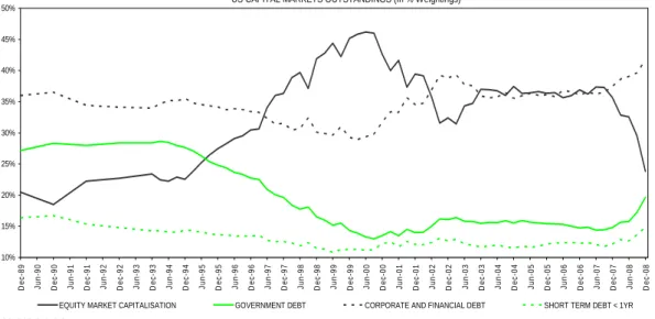
Furthermore, I have developed a U.S. capital markets portfolio proxy (CMP) comprised of equities, government debt, corporate and financial debt and money markets. Based on information available from Standard and Poor’s (2007), about the equity market capitalisation, and from BIS (2009), about the different types of debt outstanding by U.S. domestic issuers, both in US$, I considered different weightings since 1989, according to the quarterly information available. Figure 4 shows the average weightings of each asset class between 1989 and 2008, with equities and corporate and financial debt reaching 70% (35% each) of CMP. Government debt represents 18% and the short-term debt the remaining 12% of CMP. Figure 5 represents the historical evolution of percentages in each asset class and Appendix 2 includes the historical evolution in terms of US$ figures outstanding.
US CAPITAL MARKETS OUTSTANDINGS - % AVERAGE WEIGHTINGS (DEC/1989 - DEC/2008)
18% 12%
35% 35%
0% 5% 10% 15% 20% 25% 30% 35% 40%
EQUITY MARKET CAPITALISATION** CORPORATES + FINANCIALS DEBT*** GOVERNMENT DEBT*** DEBT UP TO ONE YEAR****
* US Capital Markets outstandings considering the following Asset Classes: Equities, Government Debt, Corporate and Financial Debt and Short Term Debt (Governments, Corporates and Financials); ** Equity Market Capitalisation of S&P 500. Source: S&P;
*** Outstanding Domestic Debt Securities. Source: BIS Quarterly Review Jun/2009;
**** Outstanding Domestic Debt Securities of Governments, Corporates and Financials Issuers with remaining maturity up to one year. Source: BIS Quarterly Review Jun/2009; Data available on an annual frequency between 1989 and 1992, On a quarterly frequency since Dec/1992.
US CAPITAL MARKETS OUTSTANDINGS (In % Weightings) 10% 15% 20% 25% 30% 35% 40% 45% 50% De c -8 9 J un-9 0 De c -9 0 J un-9 1 De c -9 1 J un-9 2 De c -9 2 J un-9 3 De c -9 3 J un-9 4 De c -9 4 J un-9 5 De c -9 5 J un-9 6 De c -9 6 J un-9 7 De c -9 7 J un-9 8 De c -9 8 J un-9 9 De c -9 9 J un-0 0 De c -0 0 J un-0 1 De c -0 1 J un-0 2 De c -0 2 J un-0 3 De c -0 3 J un-0 4 De c -0 4 J un-0 5 De c -0 5 J un-0 6 De c -0 6 J un-0 7 De c -0 7 J un-0 8 De c -0 8
EQUITY MARKET CAPITALISATION GOVERNMENT DEBT CORPORATE AND FINANCIAL DEBT SHORT TERM DEBT < 1YR SOURCE: S&P, BIS
Figure 5: U.S. capital markets portfolio proxy (%) historical evolution
3.3 VOLATILITY MEASURES
Analysts and financial markets participants estimate volatility in one of two following ways.
The first one is by computing the historical financial instrument (Xt)
volatility, using the standard deviation measure. Considering p and t pt−1 the
security prices in periods t and t-1, respectively, the variable of interest (Xt) is the
compounding rate of change in price between two time periods, expressed as follows
Xt =100 [ ( /∗ Ln p pt t−1)] (2)
Historical volatility calculation refers to a certain time period (e.g. daily) that can be easily transformed into any periodicity through multiplication by the square root of the number of trading days, assuming that the logarithmic changes are independent and identically distributed (IID). Also, because historical volatility always refers to a period in the past can therefore be easily calculated via the
method described above. The pendant for any time frame in the future is usually referred to as realised volatility.
The second method is to estimate a financial instrument volatility using derivatives observed prices (like options). Volatility calculated using this approach is called implied volatility and it captures the expectation of financial markets about realised volatility, for any period in the future. Unlike historical volatility, implied volatility is the reflection of the realised volatility implied from Black-Scholes option pricing model, using the options premiums observed in the market. The underlying periodicity for implied volatility is one year, as it is expressed as volatility per annum, but also, can easily be transferred into any other time periods as mentioned above.
Since capital markets and instruments are considered forward looking variables of the state of the economy, the volatility measure to adopt in order to investigate the interaction with economic growth, could be an estimation of implied volatility. However, there are important caveats. It has to be assumed that the option pricing model is correct and this type of models usually assume that volatility is constant over the life of the option, which in turn makes more difficult to interpret an implied volatility output. Also, Ang et al. (2006) raise a concern about implied volatility measures because it combines both expected volatility and the volatility risk premium. Finally, there is only historical data available for implied volatility in some asset classes, like equities. In this case, the Chicago Board Options Exchange introduced the CBOE Volatility Index, VIX, which is the benchmark for U.S. equity market volatility, with quotes only existing from 1986. Based on options on the S&P 500, it estimates the expected volatility from prices of equity index options in a wide range of strike prices, and derives expected volatility by averaging the weighted prices of out-of-the money calls and puts.
In the case of the U.S. government bonds asset class, an index followed by market participants is the Deutsche Bank U.S. Volatility Gamma Index (DGX), which consists of weighted averages of at-the-money swaptions premiums with the underlying swap maturity ranging from 3 months to 30 years. The historical data available of this index, which begins in the 1994, is not enough to analyse the
interaction of this gauges and different phases of U.S. business cycles. In addition to this, in the case of the corporate bond market it is even more difficult to find a measure of implied volatility, with a wide historical time-length and of general acceptance of market participants.
Since several asset classes are considered in the analysis (equity, government bond yields, corporate bond yields and money markets) and given the caveats of implied volatility explained above, the default measure used for all the asset classes is the historical volatility. However, empirical analysis is also done with implied volatility in the case of equities, given the constraints already exposed. Historical volatility for equities is estimated by computing the annualised standard deviation of the last twelve months rolling natural logarithm returns.
3.3.1 Yield Volatility
For interest rates and yields, although there is no consensus agreement on how volatility should be defined, according to Rieger et al. (2007), market participants should use a metric of normalised volatility. The volatility measures introduced above refer to percentage changes of some underlying asset and not to absolute changes. In the fixed income camp, the volatility on percentual changes is known as yield volatility, whereas the volatility on absolute changes (∆y) is known as normalised volatility. In this analysis, I adopted the standard deviation of the absolute rate of changes instead of relative rate of changes. This choice is warranted by three observations: (a) the risks assumed by bond market investors are proportional to the volatility of absolute rate of changes since the return on a portfolio of bonds approximately equals its modified duration times the interest rate change; (b) changes in percentual yield volatility will much depend on outright yield levels and will not be considered a pure reflection of volatility related changes; (c) in the sample there could be instances of zero rates, in which case relative changes can not be defined.
3.3.2 Capital Markets Portfolio Proxy (CMP) Volatility
In order to calculate the impact of U.S. capital markets volatility in economic growth, considering several asset classes simultaneously, I developed the intuition of the capital markets portfolio proxy (CMP) and the diversification effects that emerge in terms of overall volatility. According to the Modern Portfolio Theory, whereas the expected returns on a securities portfolio is the weighted average of expected returns on the individual assets, the same is not true for variance. The volatility of a portfolio is typically less than the weighted average of the individual volatilities. This is the gain from portfolio diversification. Consequently, the smaller the correlation coefficients the greater the benefits from diversification will be.
Considering r as the (Nx1) vector of returns on the N asset classes in time t t
The covariance matrix of asset class returns is defined as
, , , ( , ) t i t j t ij t V C o v r r σ ⎛ ⎞ ⎜ ⎟ = = ⎜ ⎟ ⎜ ⎟ ⎝ ⎠ M L L M
The (Nx1) vector of CMP weights is
1, , t t N t w w w ⎛ ⎞ ⎜ ⎟ = ⎜ ⎟ ⎜ ⎟ ⎝ ⎠ M The return on CMP is
rC M P t, = w rt t′
(3)
1 , , t t N t r r r ⎛ ⎞ ⎜ ⎟ = ⎜ ⎟ ⎜ ⎟ ⎝ ⎠ M
Hence, the variance of rCMP t, will be given by 2 , [ ] CMP t Var w rt t w V wt t t σ = ′ = ′ (4) And volatility by σC M P t, = w V wt′ t t (5) Where
N is the number of asset classes in the CMP (Equities, Government Debt, Corporate and Financial Debt, Money Markets)
, i t
r is the monthly log return of asset class i in month t ,
ij t
σ is the covariance between log return of asset class i and log return of asset class
j, in month t ,
i t
w is the weight of asset class i in CMP, in month t
The volatility of CMP is calculated in line with equation (5). For each time
period, month t, variance of asset class i and covariance between asset classes i and
j are computed based on their last twelve months log returns. Weights in t, for the
asset class i, are function of the average of the last twelve month observations,
starting in December, 1989. Due to the lack of availability of BIS data, with regard to debt outstanding before this period, I considered fixed weights for the different asset classes, between January, 1963 and December, 1989.
3.4 ECONOMETRIC MODELS
To investigate the dynamics between the U.S. capital markets and COI YoY, I have estimated standard OLS regressions using EVIEWS software. Not only were tested contemporaneous relations, but also 12 leads and lags (one year gap) of volatility of the different asset classes and CMP, as the explanatory variable, against COI. I also computed cross-correlations up to 60 months (5 years) to detect long lag-lead correlations between the two variables across different business and capital markets cycles, which results, when statistically significant, are presented in Appendix.
Since heteroscedasticity is a common phenomenon in this type of statistical relationships, White´s tests were performed in every estimated model analysis, and the results were conclusive in terms of evidence of heteroscedasticity, meaning that it was not plausible to assume that the variance of the errors was constant. By the same way, I also tested whether the residual series from the estimated models were autocorrelated, via Durbin-Watson first order autocorrelation tests, and, as in the case for heteroscedasticity, the residuals from the regressions appeared to be correlated. According to Brooks (2002), the consequences of ignoring heteroscedasticity and autocorrelation of the residuals are that the OLS coefficients of the volatility variables are not the Best Linear Unbiased Estimators (BLUE), which could lead to wrong inferences made about asset class volatility being or not an important determinant of variations in U.S. economic growth. Consequently, given the presence of both residual heteroscedasticity and autocorrelation, the t-statistics of the original regressions were appropriately changed using Newey-West modified consistent standard error estimates.
For the full-sample or sub-sample periods considered
COI YoY
_
t= +
α β
*
CM Vol
_
t i i+ −/+
u
t (6)
COI YoY
_
t= +
α β
*
CM Vol
_
t+
δ
*
D
t i i+ −/+
u
t (7)Where
α - Intercept parameter;
COI_YoY - Natural log year-over-year returns of Conference Board Coincident Indicator;
β - The slope coefficient of the explanatory variable;
_
CM Vol - 12-month rolling historical annualised volatility of natural logarithm monthly returns of equities and of capital markets portfolio proxy, or 12-month rolling historical annualised volatility of first differences of short-term yields, long-term government bond yields, corporate and financial bond yields and corporate and financial yield spreads;
D - Dummy variable taking the value 1 or 0, to represent a particular observation either having or not a given property: NBER recession periods, uptrend and downtrend economic growth periods;
δ - Dummy variable coefficient representing a shift in the intercept of the regression line due to the presence of a given property;
ε - Gaussian variable independently and identically distributed with 0 expectation
and variance σ2;
/ i i
+ − - Monthly leads/lags, up to 12, applied to the explanatory continuous and