Exploring Different Normalization and
Classification Approaches for
Mammography Analysis with CNNs
Ana C. Perrea,1, Lu´ıs A. Alexandreband Lu´ıs C. Freirec
aFaculdade Ciˆencias da Sa´ude, Universidade da Beira Interior and Instituto de
Telecomunicac¸˜oes, Covilh˜a, Portugal
bDepartamento de Inform´atica, Universidade da Beira Interior and Instituto de
Telecomunicac¸˜oes, Covilh˜a, Portugal
cEscola Superior de Tecnologia da Sa´ude de Lisboa, Instituto Polit´ecnico de Lisboa,
Lisboa, Portugal
Abstract. In order to improve the performance of Convolutional Neural Networks (CNN) in the classification of mammographic images, many researchers choose to apply a normalization method during the pre-processing stage. In this work, we aimed to assess the impact of 6 different normalization methods in the classifica-tion performance of 2 CNNs. We have also explored 5 classifiers, being the first one the CNN itself. The other 4 correspond to Support Vector Machine (SVM), Random Forest (RF), Simple Logistic (SL) and Voted Perceptron (VP) classifiers, all of them fed with features extracted from one of the layers - comprised between the sixteenth and the nineteenth - of the CNN. The last 3 classifiers were tested with different options for data testing presentation, according to the Weka software: Supplied Test Set(STS), 10-fold Cross Validation (10-FCV) and Percentage Split (PS). Results indicate that the effect of image normalization in the performance of the CNNs depends on which network is chosen to make the classification; besides, the normalization method that seems to have the most positive impact is the one that subtracts to each image the corresponding image mean and divide it by the standard deviation (best AUC mean values were 0.786 for CNN-F and 0.790 for Caffe; the best run AUC values were, respectively, 0.793 and 0.791. Layer 1 freez-ing decreased the runnfreez-ing time and did not harm the classification performance. Regarding the different classifiers, CNNs used alone with softmax yielded the best results, with the exception of the RF and SL classifiers, both using the 10-FCV and PS options; however, with these options, we cannot guarantee that the test set images are presented for the first time to the network.
Keywords. Breast Cancer, Mammography, Image Normalization, Convolutional Neural Network, Support Vector Machine.
1. Introduction
Mammographic images are usually interpreted by highly trained radiologists. However, due to the frequent need of analyzing large amounts of images that are produced on a
daily basis in medical institutions, they may misinterpret between normal and abnormal tissues [1]. Therefore, it is important to develop automatic or semi-automatic computer-assisted tools that can help radiologists in the detection and interpretation of suspicious regions on mammograms [2]. Convolutional Neural Networks (CNN) have recently been successfully used in the medical field for detection and classification of mammographic lesions [2,1,3].
To improve the performance of CNNs in this task, many researchers choose to apply a normalization method to the mammographic images during the pre-processing stage [1], which is justified by the fact that images are obtained with different exposure condi-tions and are affected by noise and some artifacts[2]. Furthermore, to perform an accurate analysis, it is necessary to achieve an optimal image contrast [2].
In the paper of [4], the authors found that the use, or not, of a pre-processing image normalization method could yield different classification results. Therefore, in this pa-per, we intend to deepen the understanding on the impact of normalization in the clas-sification performance by using 6 different image normalization methods, being the first four methods variations of Global Contrast Normalization (GCN). Therefore, we have: (method 1) subtracting the image mean; (method 2) subtracting the image mean and di-viding by the standard deviation; (method 3) histogram equalization; (method 4) his-togram equalization in combination with method 2. (method 5) and (method 6) used the same GCN applied in methods 1 and 2, respectively, in combination with a local con-trast normalization (LCN). Lastly, we tested the classification process on the same im-ages without normalization, which we call ”NoNORM” - see fig. 1 and 2. We have also explored several classifiers, being the first one the CNN itself. The other 4 correspond to Support Vector Machine (SVM), Random Forest (RF), Simple Logistic (SL) and Voted Perceptron (VP) classifiers, all of them fed with features extracted from one of the layers - comprised between the sixteenth and the nineteenth - of the CNN. The last 3 classifiers were evaluated with different options for data testing presentation, according to the Weka software [8]: Supplied Test Set (STS), 10-fold Cross Validation (10-FCV) and Percentage Split(PS).
2. Related Work
Rouhi et al. [2] used local area histogram equalization, which stretches the intensity of image pixels to extend the contrast, and then the median filtering, which is a nonlinear operation used to reduce noise (”salt and pepper” and speckle noise).
In Jiao et al. [1], the authors use mammographic images that have been normalized and whitened; the dataset was normalized to the range [0,1] by subtracting the mean and, in a subsequent step, they used a method named PCA whitening by dividing the standard deviation of its elements.
Arevalo et al. [3] applied two normalization types: (1) Global Contrast Normaliza-tion, by subtracting the mean of the intensities in the image to each pixel (the mean is calculated per image, not per pixel), and (2) Local Contrast Normalization, which mim-ics the behavior of the visual cortex and reduces statistical dependencies; the outcome is a greater difference between input features, which accelerates gradient-based learning.
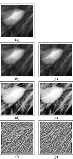
(a)
(b) (c)
(d) (e)
(f) (g)
Figure 1. Examples of the same crop image (benign lesion) with the different normalization methods: (a) NoNORM and (b-g) Methods 1 to 6.
3. Material and Methods
The dataset used in this work was the BCDR-FM dataset (Film Mammography Dataset) from Breast Cancer Digital Repository2. The downloaded subset, named BCDRF03
-”Film Mammography Dataset Number 3”, comprises 736 grey-level digitized mammo-grams (426 benign and 310 malign mass lesions) from 344 patients. These are distributed into Medio-Lateral Oblique (MLO) and Cranio-Caudal (CC) views with image size of 720×1168 (width×height) pixels and a bit depth of 8 bits per pixel in TIFF format [3].
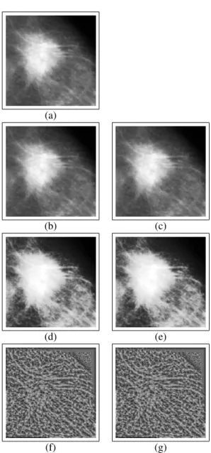
(a)
(b) (c)
(d) (e)
(f) (g)
Figure 2. Examples of the same crop image (malign lesion) with the different normalization methods: (a) NoNORM and (b-g) Methods 1 to 6.
In the pre-processing stage, we cropped ROI’s of 150×150 pixels - following the indications in [3] - using the information of the bounding box of the segmented region and preserving the aspect ratio, even when the lesion’s dimensions were bigger than 150×150). We have also performed data augmentation by using a combination of flip-ping and 90, 180 and 270 degrees’ rotation transformations.
The networks tested in this work were previously used for classifying the ImageNet ILSVRC challenge data: the CNN-F model [5] and the Caffe reference model. The archi-tecture of the CNN-F model consists in 8 learnable layers (5 convolutional layers and 3 fully-connected layers) [5]. Caffe trains models using a standard stochastic gradient
de-scent algorithm [6], and yielded the best classification performance in [4] work. In order to apply the pre-trained model to our problem, we have adapted the software MatCon-vNet [7] available for Matlab (System Specifications: Matlab R2015a and Intel i7-3820 CPU @ 3.60GHz with 32GB RAM).
Images were divided into 60% for training and validation and 40% for testing (taking into account that images from the same patient are placed only in one group), with an input size of 224×224 pixels (which is the size used by MatConvNet). The parameters’ exploration space comprised three fully connected layers and five learning rate (lr) values (1e-2, 1e-3, 1e-4, 5e-2, 5e-3 and 5e-4). We have also frozen the first convolutional layers to assess the impact in the classification performance and running time.
After the normalization and freezing tests, we applied the Caffe reference model to the normalized images with method 2 and extracted the activation’s from one of the layers comprised between the sixteenth to the nineteenth layer of the CNN. The extracted activation’s were subsequently used to apply a Support Vector Machine (SVM) classifier, based on [3], since they considered that SVM had better performance as classifier than the Softmax normally used with CNN. After that, using the activations of the layer that yielded the best results, we applied the 3 other classifiers (RF, SL and VP) using the software Weka - Waikato Environment for Knowledge Analysis, Version 3.8.1 [8].
4. Results and Discussion
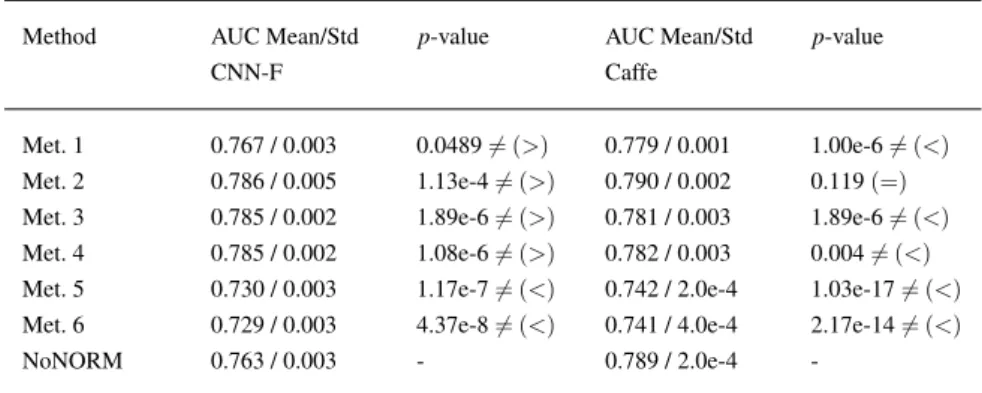
Table 1 shows the results of normalization tests, performed five times, with the CNN-F and Caffe reference models, both in terms of area under the curve (AUC) mean and standard deviation. It also includes the statistic values (p value) for comparison between the use, or not, of the different normalization methods. Note that only for Caffe and Method 2, the AUC value is statistically equal (p value = 0.119); for the others, one observes always a significant difference - for better or for worse - on the performance. The best result achieved was 0.786 with CNN-F and 0.790 with Caffe, both using Method 2. However, note that with Caffe, the difference in the results between Method 2 and the one without normalization is not significant (p value = 0.119), which raises the question if it is necessary to make the image normalization. However, in the case of CNN-F, the AUC mean value, obtained with Method 2, reveals a significant improvement in the results, from 0.763 to 0.786 (p value = 2.28e-5), with a best run of 0.793 against 0.768.
The histogram normalization method does not seem to improve the performance of the network with Caffe; however with CNN-F, one observes an increase in the classi-fication performance, although the results are slightly lower than those obtained with Method 2. While GCN seems to have some effect in the network performance, mostly in CNN-F, the LCN does not produce any improvement in the results; the best AUC mean value for these methods is 0.742. The AUC mean values for Methods 5 and 6 are similar. Table 2 shows the AUC value and running time of frozen layers tests for the best method used before (Method 2). Note that, for example, when the first layer was frozen, the AUC values did not decrease but the running times were lower (28.14 to 27.84 in CNN-F and 25.03 to 24.87 in Caffe). For CNN-F, the best AUC result was achieved with layer 2 freezing with high running time and for Caffe with layer 1 freezing with low running time.
Table 3 shows the results of the SVM classification with activation’s extracted from the sixteenth to the nineteenth layers of the CNN, obtained with Caffe for normalization
Method AUC Mean/Std p-value AUC Mean/Std p-value
CNN-F Caffe
Met. 1 0.767 / 0.003 0.0489 6= (>) 0.779 / 0.001 1.00e-6 6= (<) Met. 2 0.786 / 0.005 1.13e-4 6= (>) 0.790 / 0.002 0.119 (=) Met. 3 0.785 / 0.002 1.89e-6 6= (>) 0.781 / 0.003 1.89e-6 6= (<) Met. 4 0.785 / 0.002 1.08e-6 6= (>) 0.782 / 0.003 0.004 6= (<) Met. 5 0.730 / 0.003 1.17e-7 6= (<) 0.742 / 2.0e-4 1.03e-17 6= (<) Met. 6 0.729 / 0.003 4.37e-8 6= (<) 0.741 / 4.0e-4 2.17e-14 6= (<)
NoNORM 0.763 / 0.003 - 0.789 / 2.0e-4
-Table 1. Results of normalization tests with the CNN-F and Caffe reference models (AUC mean and standard deviation values) and statistic values of comparison between the use, or not, of the different normalization methods (p value).
Frozen Layers CNN-F AUC / Time Caffe AUC / Time
No 0.781 / 28.14 0.790 / 25.03 1 0.782 / 27.86 0.798 / 24.87 2 0.789 / 28.84 0.771 / 27.21 3 0.781 / 30.04 0.788 / 24.99 1 and 2 0.767 / 29.15 0.773 / 25.33 1 and 2 and 3 0.759 / 27.56 0.750 / 24.88 1 and 3 0.779 / 27.85 0.793 / 26.91 2 and 3 0.786 / 29.36 0.763 / 25.07
Table 2. Results of frozen convolutional layers tests (performed one time) with CNN-F and Caffe for Method 2 (lr 5e-3) in terms of AUC and running time, in minutes.
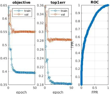
Method 2 (lr 5e-3, performed five times). The AUC mean value obtained from the CNN classification was 0.791, with a standard deviation of 0.002. Fig. 3 shows the graphics (Objective, Top1err and ROC) for the best run, with an AUC value of 0.794. With this approach, we match the result of 0.79 obtained by [3] with the combined use of DeCAF (an old version of Caffe), normalized images and an SVM instead of the Softmax layer, since they considered that the former had better performance as classifier than the latter. Note that the best result yielded by the SVM (AUC mean = 0.773) was obtained using the features from the sixteenth layer. However, the overall performance was lower than the one obtained only with CNN, which does not agree with the work of [3].
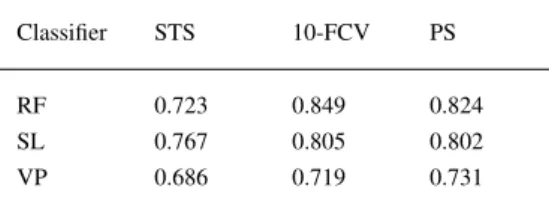
Table 4 shows the AUC mean results for the RF, SL and VP classifiers, all of them conducted with the 3 different data presentation options (STS, 10-FCV and PS). Note that the results differ substantially depending on the classifier/option combination; the best results were obtained with the RF/10-FCV combination (AUC mean value = 0.849) but, in our opinion, the use of STS is the most correct because only with this approach we can ensure that the network never sees crops from a given image both in the train and test sets, whereas with 10-FCV and PS, different crops from a given image can appear in both the train and test sets. However, the STS led to the worst results, being its best
Figure 3. Objective, Top1err and ROC curve graphics for the best run with Caffe for Method 2 (lr 5e-3) with an AUC value of 0.794
Table 3. SVM classification mean results obtained with different activation layers from the Caffe model, all with Method 2 (mean values calculated from five runs).
Act. Layer Dimension AUC mean AUC Std
16 80 Mb 0.773 0.003
17 60 Mb 0.769 0.002
18 80 Mb 0.762 0.004
19 49 Mb 0.752 0.003
AUC mean value of 0.767 with SL. These results can eventually explain the disparity of values obtained by different researchers.
5. Conclusions
Taking into account the dataset (the same used only in the work of [3]), the effect of im-age normalization in the performance of the CNNs depends on which network is chosen to make the lesion classification. Our results indicate that, for Caffe, the image normal-ization is not as important as for CNN-F.
The networks do not have the capability to normalize the input data, however they are capable to find the most suitable filters to apply in the different sets of images used
Table 4. AUC mean results for RF, SL and VP classifiers, obtained using the activations from the sixteenth layer of the Caffe model and Method 2 (mean values calculated from five runs).
Classifier STS 10-FCV PS
RF 0.723 0.849 0.824
SL 0.767 0.805 0.802
VP 0.686 0.719 0.731
as input. In some cases, image normalization may not be necessary whereas, in others, its use can lead to an increase in the performance of the network. The method of image normalization that seems to have the biggest positive impact in the classification perfor-mance is the one that subtracts the image mean and divides by the standard deviation (Method 2); on the contrary, the use of LCN is associated with the worst results.
The freezing of layer 1 resulted in an improvement both in terms of AUC and com-putation time, for both tested networks. Since the first layers of the networks learn sim-ple and generic characteristics of the data, such as edges or corners, depending on which layer the freezing option is used, the performance of the network will not decrease and the computational time can be lower.
The results obtained with SVM were worse than the ones yielded by the CNN alone (with the Softmax as classifier) for all the different layers. However, the best result was achieved using the activations from the sixteenth-layer of the CNN (AUC mean value = 0.773). Poor results were also observed with the other 3 classifiers for the STS data presentation option, with the best AUC mean value of 0.767. The use of 10-FCV and PS options, both with RF, yielded the best AUC mean values of this work (respectively 0.849 and 0.824), but without the guarantee that crop images are not shared by the training and testing sets.
In this paper, all the classifications were made using the dataset of one of the works referenced in the state-of-the-art section. In future work, we intend to expand our analysis in order to compare against other datasets and, by doing so, we hope it will facilitate the direct comparison against other approaches.
References
[1] Jiao, Z., Gao, X., Wang, Y., Li, J.: A deep feature based framework for breast masses classification. Neurocomputing.197, 221–231, 2016.
[2] Rouhi, R., Jafari, M., Kasaei, S., Keshavarzian, P.: Benign and malignant breast tumors classification based on region growing and CNN segmentation. Expert Systems with Applications.42, 990–1002, (2015.
[3] Arevalo, J., Gonz´alez, F.A., Ramos-Poll´an, R., Oliveira, J.L., Guevara Lopez, M.A.: Representation learning for mammography mass lesion classification with convolutional neural networks. Computer Methods and Programs in Biomedicine 127, 248–257, 2016.
[4] Perre, A., Alexandre, L.A., Freire, L.C.: Lesion Classification in Mammograms Using Convolutional Neural Networks and Transfer Learning. VI ECCOMAS Thematic Conference on Computational Vision and Medical Image Processing, VipIMAGE, 2016.
[5] Chatfield, K., Simonyan, K., Vedaldi, A., Zisserman , A.: Best Scientific Paper Award Return of the Devil in the Details: Delving Deep into Convolutional Nets British Machine Vision Conference, 2014. [6] Jia, Y., Shelhamer, E.. Donahue, J., Karayev, S., Long, J., Girshick, R., Guadarrama, S., Darrell, T.:
[7] Vedaldi, A., Lenc, K.: MatConvNet – Convolutional Neural Networks for MATLAB. Proceeding of the ACM Int. Conf. on Multimedia, 2015.
[8] Frank, E., Hall, M.A., Witten, I.H.: The WEKA Workbench. Online Appendix for ”Data Mining: Prac-tical Machine Learning Tools and Techniques”, Morgan Kaufmann, Fourth Edition, 2016.