Aircraft Attitude Tracking using a Model Reference Adaptive Control

(1)

UNIVERSIDADE DA BEIRA INTERIOR

Engenharia

Aircraft Attitude Tracking using a Model

Reference Adaptive Control

(versão corrigida após defesa)

Emanuel da Costa Castanho

Dissertação para obtenção do Grau de Mestre em

Engenharia Aeronáutica

(ciclo de estudos integrado)

Orientador: Prof. Doutor Kouamana Bousson

(2)

(3)

Dedication

To my parents, Eduardo Castanho and Virgínia Costa, for helping me both emotionally and financially even miles away. The fact that they believed in my learning potential was essential in order to achieve this long academic journey.

To my two sisters, Marina and Teresa, for all their support.

(4)

(5)

Acknowledgments

First, I would like to thank my academic supervisor Dr. Kouamana Bousson for suggesting me a very interesting, yet challenging, dissertation theme. His knowledge sharing, motivational speeches, as well as his humor and respect for the students were a great help to keep the focus and the calm during the realization of this thesis.

Secondly, I am grateful to all the educational establishments and professors who, over the years, have helped me in some way to build my intellectual personality, allowing me to be where I am today.

Finally, I would like to thank some colleagues for sharing useful engineering and aeronautical information.

(6)

(7)

Resumo

O controlo de voo de aeronaves é um assunto importante e interessante, no qual uma ampla gama de habilidades e esforços de engenharia são alinhados, a fim de projetar um controlador capaz de garantir estabilidade, evitar ocorrência de falhas e em certos casos contribuir para um voo completamente autónomo. Durante o voo, uma aeronave apresenta um movimento tridimensional combinado que pode ser decomposto em um movimento simétrico ou longitudinal no eixo de arfagem e um movimento assimétrico ou latero-direcional nos eixos de rolamento e guinada.

Na presente dissertação é efetuado o controlo da atitude de uma aeronave, em que um controlo adaptativo por modelo de referência (MRAC) discreto com algoritmo de traço constante é aplicado a um F-4C Phantom, cujo modelo é obtido por identificação de sistema através de dados gerados pelas equações de estado linearizadas para o caso longitudinal e latero-direcional. O objetivo é testar o desempenho desse tipo de controlo durante condições específicas de voo.

No caso longitudinal, a aeronave é assumida como sendo um sistema de única entrada e única saída (SISO) e são realizadas simulações para dois exemplos de dados de ângulo de arfagem, nos quais duas expressões para o controlador (clássica e penalizada) são aplicadas em cada exemplo para comparar o seu desempenho.

No caso latero-direcional, a aeronave é assumida como sendo um sistema de múltipla entrada e múltipla saída (MIMO) com número de entradas igual ao de saídas, em que o algoritmo do MRAC deve ser modificado de modo a descrever um processo de desacoplamento. Foram realizadas simulações para verificar se o controlador é capaz de lidar com a relação de acoplamento entre variáveis, como velocidade lateral, ângulo de rolamento, ângulo de aileron e ângulo do leme de direção.

O tipo de controlo adaptativo estudado apresentou bons resultados nos dois casos de estudo, seguindo o sinal de referência sem discrepâncias. A escolha das condições iniciais da simulação também é analisada nesta dissertação a fim de evitar saturação dos atuadores.

Palavras-chave

(8)

(9)

Abstract

A discrete-time explicit Model Reference Adaptive Control (MRAC) with constant trace algorithm is applied to a linearized aircraft model during longitudinal and lateral-directional motions in order to test the performance of this type of control during specific flight conditions. The model was obtained through system identification with data generated from the linearized state equations of the F-4C.

In the longitudinal case the aircraft behaves like a Single-Input-Single-Output (SISO) system and simulations are performed for two examples of pitch angle data, in which two expressions for the control (classic and penalized) are applied in each example to compare their performance.

In the lateral-directional case the airplane behaves like a Multi-Input-Multi-Output (MIMO) system with equal number of inputs and outputs and the MRAC control law must be modified to describe a decoupling process. Simulations are performed in order to verify if the controller is able to handle the coupling relation between some variables, such as lateral velocity, roll angle, aileron angle and rudder angle.

The adaptive control in both study cases and for the chosen initial conditions showed good tracking when following the reference output, presenting no drift problems. The choice of the initial simulation conditions is also analyzed, in order to prevent actuator saturation.

Keywords

(10)

(11)

List of Figures

Figure 1.1 – Generalized body axis and positive notation. ... 1

Figure 1.2 – Typical MRAC scheme. ... 4

Figure 1.3 – North American X-15 number 3. ... 5

Figure 1.4 – McDonnell Douglas X-36. ... 6

Figure 2.1 – Direct relation between variables. ... 9

Figure 2.2 – Coupling relation between variables. ... 10

Figure 4.1 – McDonnell Douglas F-4C Phantom II. ... 19

Figure 4.2 – Elevator angle perturbation over time. ... 23

Figure 4.3 – Pitch angle perturbation generated. ... 24

Figure 4.4 – Aileron angle perturbation over time. ... 25

Figure 4.5 – Rudder angle perturbation over time. ... 25

Figure 4.6 – Roll angle perturbation generated with and without noise. ... 26

Figure 4.7 – Lateral velocity perturbation generated with and without noise. ... 27

Figure 4.8 – Scheme to obtain the airplane model using generated data. ... 28

Figure 5.1 – MRAC scheme used in the simulation. ... 29

Figure 5.2 – Example 1 with classic control. ... 32

Figure 5.3 – Example 1 with penalized control. ... 33

Figure 5.4 – Example 2 with classic control. ... 35

Figure 5.5 – Example 2 with penalized control. ... 36

Figure 5.6 – Testing the controller with the reference data from (5.2) and (5.3). ... 38

Figure 5.7 – Testing the controller with φref from (5.2) and vrefset to 0. ... 40

(14)

(15)

List of Tables

Table 4.1 – F-4C General Specifications. ... 20 Table 5.1 – Initial conditions for longitudinal simulation. ... 30 Table 5.2 – Initial conditions for lateral-directional simulation. ... 31

(16)

(17)

Nomenclature

Symbols Description System of Units

A System matrix [−]

â, b̂, ĉ, d̂, ê, f̂, ĝ, ĥ Set of adaptive weights (they are time-varying) [−]

B Input matrix [−]

C Output matrix [−]

d Time delay [−]

F Adaptation gain matrix [−]

I Identity matrix [−]

J Cost function [−]

k Time instant, non-dimensional [−]

m Dimension of the state-space [−]

n Fixed length of the rectangular window method [−]

N Sensor noise vector [−]

p Roll rate perturbation [rad/s]

p̂ Estimation parameter vector [−]

q Pitch rate perturbation [rad/s]

r Yaw rate perturbation [rad/s]

t Time [s]

u Longitudinal velocity perturbation [m/s]

up Plant input [−]

v Lateral velocity perturbation [m/s]

w Vertical velocity perturbation [m/s]

x State vector [−]

yp Plant output [−]

Greek Letters Description System of Units

γ Weighting coefficient [−]

Δ Controllability matrix [−]

ε* “Augmented” filtered plant-model error _[−]

ζ Rudder angle perturbation [rad]

η Elevator angle perturbation [rad]

θ Pitch angle perturbation [rad]

Θ Observability matrix [−]

Λ Eigenvalue [−]

λ1, λ2 Coefficients to obtain different types of adaptation algorithms [−]

ξ Aileron angle perturbation [rad]

φ Roll angle perturbation [rad]

Φ Plant variable vector [−]

ψ Yaw angle perturbation [rad]

Others Description System of Units

(ref) Subscript to denote a reference signal [−]

(T₎ _{Superscript to denote a transposed vector/matrix} _[−]

Re Real part [−]

(18)

(19)

List of Acronyms

CG Centre of Gravity

FCS Flight Control System

LTI Linear Time-Invariant

MIMO Multi-Input-Multi-Output

MIT Massachusetts Institute of Technology MRAC Model Reference Adaptive Control MRAS Model Reference Adaptive System

NASA National Aeronautics and Space Administration PID Proportional-Integral-Derivative

SISO Single-Input-Single-Output

STR Self-Tuning Regulator

U.S. United States

UAV Unmanned Aerial Vehicle

(20)

(21)

Chapter 1 – Introduction

1.1 System of Axes and Notation

An aircraft has six degrees of freedom, being their motion described in terms of force, moment, linear and angular velocities and attitude. The attitude is defined as the angular orientation of generalized body axes with respect to earth axes [1].

In order to obtain coherent results and analyzes in the final sections of this dissertation, the system of axes considered and the positive notation of the angles for the control surfaces are shown in Figure 1.1.

Since the ailerons act differentially, ξ is considered as the mean value of the two surface angles [1].

(22)

1.2 Adaptive Flight Control

Flight vehicles, such as civilian and military aircraft, are designed to strictly follow airworthiness codes and regulations. Flight control systems are fundamental to ensure the maneuverability of the aircraft during its entire mission, being those manufactured based on modern control theory that offers a huge number of various designs and techniques [2].

Modern FCSs allow to introduce the concept of “family”, where flying different aircraft can be made almost the same for pilots, reducing pilot training costs. FCSs also help control the open-loop instability characteristic of some military aircraft, which is related to agility and high-performance [3].

An aircraft is a non-linear dynamic system that changes significantly with speed, altitude, angle of attack, fuel consumption, among other factors, and in some particular cases may be subject to structural damage and component failure [4]. During its mission, the autopilot may be subject to regimes (specified by speed and altitude) in which the aircraft can be approximated by a linear system, however this only guarantees local stability. It can be said that the autopilot must adapt to almost all conditions, so it is necessary a controller that offers good results when large uncertainties are present or when the dynamics of the system are not fully known [5], [6].

Adaptive control is useful in a practical engineering environment and is a good option to design autopilots, as it requires only a limited knowledge of the plant structure [7]. It can adjust its own operation behavior in response to unpredictable changes in the dynamics of the plant or in the operating environment [3]. This type of controller differentiates from the other types because of its adaptation mechanisms, where an online estimation of the uncertainties is done and the controller adapts their own parameters to produce an input to anticipate, minimize, or overcome the undesirable deviations from the targeted specifications [8], [9].

Adaptive controllers work to overcome slowly time varying changes of any parameters of a particular system, while fixed-gain controllers are only suitable for time-invariant systems. Furthermore, modern LTI robust controllers and other fixed-gain controllers may decay in performance due to uncertain conditions. Also, robust controllers performance may not be better than adaptive control when subjected to constant or slow varying parameters [5].

Most industrial processes in the aerospace/aeronautic sector are complex and not well understood. For instance, in some cases when an aircraft is developed and modifications are necessary, a wind tunnel might be an expensive option in terms of schedule and budget, instead an adaptive control can be retrofitted into the existing production FCS, reducing costs [6].

(23)

Adaptive controllers are normally designed using methods based on Lyapunov stability theory [10] and the way the parameter estimator is combined with the control law leads to two different approaches. The first one is indirect adaptive control or explicit adaptive control, in this approach the plant parameters are constantly estimated and used to calculate the controller parameters so that the plant can mimic the behavior of the explicit plant model. The second approach is direct adaptive control or implicit adaptive control, here an implicit plant model is parameterized directly in terms of controller parameters, that is without intermediate calculations involving plant parameter estimates [5], [11].

Two important adaptive control schemes in flight control can be built from the two approaches previously mentioned. The first one is gain-scheduling and the second one is model reference adaptive control.

Gain-scheduling is the most used method for handling parameter variations in flight control systems since it is usual for an aircraft to have acceptable flying qualities at many points in its flight envelopes [12]. In this type of control, the Mach number and the altitude are measured by sensors and stored as scheduling variables in a look-up table, then the scheme detects the operating point and chooses the corresponding value from the table to change the controller [4], [11]. Although some authors consider that gain-scheduling systems are not fully adaptive, the truth is that this type of control presents satisfactory results [13]. There are, however, flight missions where gain-scheduling cannot provide good results, such as when an aircraft has just released a significant quantity of payload or when is performing rapid maneuvers [12].

The MRAC is the basis of this dissertation, thus the next subsection is focused on this type of control.

1.2.1 The Model Reference Adaptive Control (MRAC)

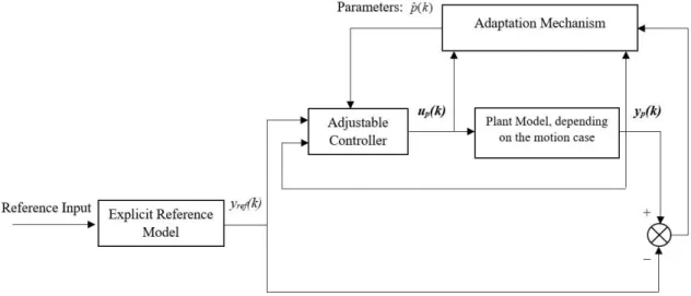
MRAC is a possible new flight control technology for aerospace vehicles in the near future [14]. This controller can be built using a direct or an indirect approach [11] and was originally proposed to solve performance specifications. The desired performance of the system is given in terms of a reference model that determines how the process output ideally should respond to an external command signal. The structure of a MRAC system includes a plant with a known structure but unknown parameters, reference model, adaptive law and controller. The adaptive law adjusts the controller’s parameters based on the tracking error between the outputs of the plant and the reference model to ensure good results [4].

Although many physical systems exhibit non-linear characteristics, most MRAC design methods assume that the control problem is linear [15]. The MRAC system has a feedback loop composed of the plant and the controller and another feedback loop that changes the

(24)

controller parameters. A typical model reference adaptive control system block diagram based on [14] is shown in Figure 1.2.

The MRAC is one of the most popular types of adaptive control [15]. Its design for MIMO plant models with multiple sensors and actuators is more complex than in the SISO case, because of the coupling between inputs and outputs. However, as in the SISO case, the design of a MRAC for a MIMO plant can be achieved by combining a control law with an adaptive law [11].

The MRAC can be used in some situations to avoid gain-scheduling and other methods, that might be time consuming, costly and labor intensive [16].

1.3 Historical Overview

The implementation of adaptive control on aircraft flight has undergone several changes over the years. In this section a brief historical introduction will be made, where the most important dates are mentioned.

The development of adaptive control emerged in the early 1950s with the aerospace industry due to the design of autopilots for aircraft that operated in a wide flight envelope, with a large range of speeds and altitudes [17].

Due to drastic changes in flight conditions it was found that ordinary constant-gain and linear feedback control only worked well in one operating condition of the whole flight regime, so a more sophisticated controller was needed. After a significant research and development, gain-scheduling control was accepted as a suitable technique for FCSs, since there was few information available about the non-linearity of adaptive control [4], [14].

In 1951, researchers successfully developed a self-optimizing controller for the combustion engine of an aircraft, and a flight test was successfully conducted. In 1958, it was proposed

(25)

led to a design rule known as “MIT rule” by Whitaker [5], [17], however this controller had some stability problems. The MRAC was an idea from the early work on flight control that had an important impact on the adaptive control discipline.

The early 1960s began very well in terms of adaptive control theory and implementation. It was shown the applications of dynamic programming in adaptive controls [18] and it was introduced the state-space system representation as well as the use of Lyapunov stability for general control systems [9]. There were also important results in stochastic control theory and developments in system identification [4].

In 1967, an intense period of research ended dramatically with a hypersonic flight tested by NASA, in which one of the three X-15 aircraft crashed, killing the test pilot Michael J. Adams. The X-15 (Figure 1.3) was using the Honeywell’s MH-96 self-oscillating adaptive controller, which had already been used in several missiles [14], [18]. Although it was an isolated case, the fatal failure of the adaptive control in combination with the success of gain-scheduling based on air data sensors casted some doubts on fully adaptation systems in practical applications, such as aircraft flight.

Research in adaptive control resurged in the 1970s, where Lyapunov stability theory was established as a foundation for model reference adaptive control and different estimation schemes were combined with various design methods. Many successful applications for MRAC and STR were reported, however theoretical results were still limited [4], [14], [18]. In 1977, the first design of a MRAC for discrete-time SISO systems in input-output form was proposed by Ionescu and Monopoli [20].

In the early 1980s, adaptive controllers started to be commercialized because of the rapid progress in microelectronics. Between the 1980s and early 1990s the robustness of adaptive controllers was addressed and studies on non-linearity with results on “feedback linearization” led to an increased understanding of adaptive control [4], [21]. Since there, engineers have been focused upon determining the stability and robustness of MIMO designs in the presence of parameter uncertainties, leading to new methods [17]. This hard work over

(26)

the years also brought the success of the X-36 aircraft (Figure 1.4) test flight which used onboard adaptive control [23].

In the 1990s it was introduced some concepts about neural networks as a mechanism for adaptation and, until the present, they are still being studied and applied [24].

NASA and other researchers have already contributed a lot to adaptive control technology development and research in this matter is still ongoing. UAV flight experiments regarding new adaptive controllers have been made, increasing the confidence in model reference adaptive control as a possible new flight control technology for aerospace vehicles in the near future [14].

Although the study of adaptive control has recently provided good experimental results in the aerospace industry, new problems arisen concerning the creation of the L1-AC in 2006-2011,

where the method’s proofs and claimed advantages were putted into question in 2013-2014 [9], [25]. The adaptive control discipline is a constantly changing field.

1.4 Main Objectives

The aerospace industry has always been an inspiration for the design of controllers leading to a great variety of them, as it was mention in the previous section. With the recent widely spread of UAVs and increasing demands on performance and reliability for autopilots during complex missions [26], adaptive control theory should be used in order to ensure satisfactory results [8], being the MRAC a possible future option.

A literature review on the field of adaptive control shows that different types of MRAC with different aeronautical applications, such as reconfigurable flight control for airplanes that suffered structural damage [27], [28] or combat aircraft that are considered highly non-linear systems [16], [29], have been already addressed. Also, the works from [3], [30]–[32] and [33]

(27)

include topics about adaptive decoupling control of MIMO plants and MRAC with lateral-directional analysis.

The main objective of this dissertation is to verify the tracking performance of a discrete-time explicit MRAC with constant trace algorithm applied to an example aircraft. This type of control is based on the work of Landau and Lozano [20] and other authors [34], [35], presenting very few results in the literature when applied to aircraft flight control.

The full aircraft motion is analyzed, and attitude flight data is generated using the F-4C Phantom’s linearized equations of motion. In the longitudinal motion case, the aircraft is assumed to be a SISO system where a classic control and a penalized one are compared in terms of operation. In the lateral-directional motion case, the aircraft is assumed to be a MIMO system and the MRAC design is slightly modified to decouple the relation between the inputs and outputs of the plant. In the first motion case, two different reference signals are used and in the last motion case, the data was generated using sensor noise.

1.5 Layout

This thesis is divided into a total of six chapters in order to provide an easy and intuitive reading:

Current Chapter - Theoretical concepts related to adaptive control are given, as well as important axes notation and main objectives of the study. A brief historical review is presented with the most important dates related to flight control in the aeronautic industry. Finally, the layout is given.

Chapter 2 – The problem is identified and explained for both motion cases. The ideal situation in contrast to reality is presented, establishing the basis for the next chapter.

Chapter 3 – It describes the MRAC algorithm in three parts. The first part is about the adaptation mechanism, the second one introduces the fundamental requirements that a system needs to fulfill to carry on with the third part that presents the control law equations. Two types of control law, classic and penalized, will be introduced. Also, a slightly modified version of the penalized control law is presented for the decoupling process of a MIMO plant.

Chapter 4 – In this section the linear case of study is described and how the flight data was generated to be used in the creation of models with system identification. It is also checked if the F-4C Phantom meets all stability, controllability and observability requirements.

Chapter 5 – The simulation, using appropriate software, is performed for the longitudinal and lateral-directional motions, where the results are shown through graphics with the concomitant analysis.

(28)

Chapter 6 – It is composed by the principal remarks, conclusions and suggestions for future studies related to the subject.

Finally, all the used bibliography and some appendix (including two papers) with relevant information are presented.

(29)

Chapter 2 – Problem Statement

2.1 Longitudinal Motion

Every pilot wants an accurate aircraft that can be effectively controlled during the path between its point of departure and its destination. However, the path of any aircraft is never completely stable without control. In order to fly a straight and level route, continuously controlling adjustments must be made, either through a human pilot or by an automatic FCS. Small corrections during several hours of flight can be exhausting for a pilot, so automatic control is a good flight implementation [12].

Usually, for study purposes and under specific conditions, a plant can be described by a set of LTI differential equations with the following state-space form:

( )

p p

x t

Ax t

Bu

t

y

t

Cx t

N t

=

+

=

+

(2.1)

In this longitudinal motion study, the plant is an airplane with input (

u

_p



): elevator angle; and output (

y

_p



): pitch angle. The engine thrust is held constant and the other output variables are not analyzed. In Figure 2.1, this paragraph is translated schematically.

Where, at each time instant, the longitudinal model is given by:

ˆ

( )

T

(

1)

(

1)

p

y

k

=

p

k

−   −

k

(2.2) with: 0

ˆ

1

ˆ

1 0 1

ˆ

T

( )

[ ( ),...,

_n

( ),

ˆ

( ),...,

ˆ

_n

( )]

p

k

=

b k

b

₋

k a k

a

₋

k

(2.3) 0 0

ˆ

T

( )

[

( );

ˆ

T

( )]

p

k

=

b k p

k

(2.4) 0

( )

[

(

1),...,

(

1),

( ),...,

(

1)]

T p p p p

k

u

k

u

k

n

y

k

y

k

n



=

−

− +

(2.5)

(30)

0

( )

[

( );

( )]

T T p

k

u

k



=



(2.6)

Given the measurements (Φ0), the parameter vector should be estimated, and the

appropriate control determined so that it tracks the desired reference. Since the plant has only one input and one output, this problem can be considered as SISO, being the solution presented in chapter 3 through a control algorithm. This algorithm is based on the MRAC scheme for SISO plants from Landau and Lozano [20].

2.2 Lateral-Directional Motion

The ideal situation in terms of aircraft control during lateral-directional flight is that ailerons are only responsible for rolling and the rudder is only responsible for yaw, consequently changing the lateral velocity. However, in reality there is a coupling relation between those variables.

Most control systems for industrial processes are designed for SISO plants, this is acceptable only if the coupling relations between inputs and outputs are weak. Nevertheless, there are many MIMO processes that have strong coupling relations that cannot be disregarded when designing a controller. Thus, it may be desirable to design a controller with decoupling to control the multiple outputs individually [32]. This is a MIMO problem with high coupling, in which a PID and classical control methods are impractical to yield acceptable results, although being very effective when dealing with SISO systems [3], [8].

Applying a specific type of MRAC to a MIMO system is a very interesting problem since, although several adaptive controllers have been introduced in the past few years, only some of these schemes deal with the problem of decoupled control [31].

In this lateral-directional motion study, the plant is an airplane with inputs (

u

_p



2): aileron angle and rudder angle; and outputs (

y

_p



2): roll angle and lateral velocity. In Figure 2.2, it can be seen the coupling relation between the different variables of the plant, where the superscripts 1 and 2 are used to distinguish between the two relations.

(31)

Where, at each time instant, the lateral-directional model is given by: (1)

_ˆ

(1) (1)

( )

T

(

1)

(

1)

p

y

k

=

p

k

−  

k

−

(2.7) (2)

_ˆ

(2) (2)

( )

T

(

1)

(

1)

p

y

k

=

p

k

−  

k

−

(2.8)

p̂(k) and Φ(k) must translate the decoupling process of the relation between the multi-variables of the plant. Therefore, one has the following formats:

(1) 1 1 0 1 0 1 0

ˆ

T

( )

[

( ),...,

_n

( ),

ˆ

( ),...,

ˆ

_n

( ),

ˆ

( ),...,

ˆ

_n

( )]

p

k

=

d k

d

₋

k e k

e

₋

k c k

c

₋

k

(2.9) (1) (1) 0 0

ˆ

T

( )

[

( );

ˆ

T

( )]

p

k

=

d k p

k

(2.10) (1) 0 (1) (1) (2) (2) (1) (1) ( ) [ ( 1),..., ( 1), ( 1),..., ( ), ( ),..., ( 1)] T p p p p p p k = u k− u k− +n u k− u k−n y k y k− +n



(2.11) (1) (1) (1) 0

( )

[

( );

T

( )]

T p u

k



=



(2.12) (2) 1 1 0 1 0 1 0

ˆ

T

( )

[

ˆ

( ),...,

ˆ

_n

( ),

( ),...,

_n

( ),

( ),...,

_n

( )]

p

k

=

g k

g

₋

k h k

h

₋

k

f k

f

₋

k

(2.13) (2) (2) 0 0

ˆ

T

( )

[

ˆ

( );

ˆ

T

( )]

p

k

=

g k p

k

(2.14) (2) 0 (2) (2) (1) (1) (2) (2) ( ) [ ( 1),..., ( 1), ( 1),..., ( ), ( ),..., ( 1)] T p p p p p p k = u k− u k− +n u k− u k−n y k y k− +n



(2.15) (2) (2) (2) 0

( )

[

( );

T

( )]

T p u

k



=



(2.16)

Given the measurements (Φ0(1) and Φ0(2)), the parameter vectors should be estimated, and the

appropriate controls determined so that they track the desired references. The following section presents the algorithm that intends to solve the referred problem. This algorithm is based on the MRAC scheme for SISO plants from Landau and Lozano [20], being the penalized control law extended for MIMO plants.

(32)

(33)

Chapter 3 – The MRAC Algorithm

3.1 Adaptive Law

The adaptation algorithm is coupled with the control algorithm [36] and the most important requirement when designing an adaptive law is to achieve asymptotic tracking of a known reference signal with good stability [21]. The MRAC technique allows to easily incorporate considerations of decoupling in the adaptive design [28], so this algorithm is valid for a SISO and a MIMO plant.

The parameter estimation problem is dynamic and uses real-time measured data signals to identify linear model parameter estimates [4], [37], [38]. The adaptation mechanism is described next by a set of equations that estimate process parameters.

*

ˆ

( )

ˆ

(

1)

(

1)

(

)

( )

p k

=

p k

− +

F k

−  − 

k

d



k

(3.1) with: 1 1 2

1 (

1)

(

)

(

)

(

1)

( )

(

1)

;

( )

( ) /

( )

(

)

(

1)

(

)

(0)

0

T T

F k

k

d

k

d

F k

k

d

F k

k

d

F





_{−   −}

_{ }

₋

_

₋



=





− −



+ 

−



−   −











(3.2)

To make the algorithm implementable an expression for ε*_{, which depends on the parameters}

estimated up to k-1, is given as:

*

( )

ˆ

(

1)

(

)

( )

1 (

)

(

1)

(

)

T p T

y

k

p

k

d

k

d

F k

k

d



=

−

−  −

+ 

−



−  −

(3.3)

To complete the introduction of this algorithm, one needs to choose the correct values of λ1(k) and λ2(k). The constant trace algorithm [34] is used, where the ratio between λ1(k) and

λ2(k) is maintained equal to 1, while λ1 is adjusted at each time step according to:





1 ( 1) ( ) ( ) ( 1) ( 1) 1 ( ) ( 1) ( ) ( ) (0) T T F k k d k d F k tr F k k d F k k d k tr F  −   −   −  − − − +  −  −   − =













(3.4)

(34)

with:

1 2

0 



( )

k



1; 0





( )

k



2 

k

(3.5)

The parameter estimates are calculated at each time sample when new measured data are available, thus the above algorithm requires that some of the data points be stored. This recursive nature avoids reprocessing old data, ensuring an efficient operation and better results [39].

Real-time parameter estimation involves adjustment of some variables, such as the variable n, to decide how long into the past the data memory will extend. This is important because, in the context of aircraft flight, there are periods of low or no excitation where the control and state variables are almost constant, leading to numerical problems for some methods when noise is present [4], [37].

Note that, during the execution of the algorithm for a MIMO plant one must use the adaptive law two times, one to update p̂(1)_(k)_{and another to update}p̂(2)_(k)_.

3.2 Stability, Controllability and Observability

Before designing a control law, it is necessary to verify that the system to be studied has the requirements regarding stability, controllability and observability. In order to define these concepts, one must consider a system described by a set of equations as (2.1).

3.2.1 Dynamic Stability

There are essentially three methods to verify if a system is stable or not:

• Analysis of eigenvalues;

• Use of Lyapunov’s stability theorem; • Use of Jane Cronin’s theorem.

In the present dissertation, only the first method is used in which the system from (2.1), considering up=0, is dynamically stable around equilibrium if and only if all eigenvalues of A

have negative real parts, Re(Λ)<0. If there is an eigenvalue with positive real part, then the system is unstable.

If all the eigenvalues have non-positive real parts and at least one of them have a zero real part, then the matrix A is a critical matrix and the equilibrium of the system can be marginally stable [40].

(35)

3.2.2 Controllability of Dynamic Systems

The system from (2.1) is said to be controllable if it is possible by means of an unconstrained controller to guide the physical system between two arbitrarily specified states in a finite period of time [41].

With the characterization by Kalman [40], it is possible to find if a dynamic system is controllable using the controllability matrix:

2 1

,

,...,

m

B AB A B

A

−

B





 = 



(3.6)

The system will be controllable if and only if, the rank of the controllability matrix is m, i.e.: rank(Δ)=m.

3.2.3 Observability of Dynamic Systems

The dynamic system from (2.1) is observable, if for any t>0, the initial state can be determined by the control input behavior and the output in the interval [0,t]. In other words, the system is observable if, for any sequence of state and control vectors, the current state can be determined in a finite period of time using only outputs [41].

With the characterization by Kalman [40], it is possible to find if a dynamic system is observable using the observability matrix:

2 1 m

C

CA

−

















 =

















(3.7)

(36)

3.3 Control Law

While the controlled system is operating, it is important that the adaptive law updates in real-time the controller parameters, so that the control law achieves tracking stability and performance goals, matching the plant output with the reference output [4], [34], [38].

Two types of control law are introduced in this section. They will be later compared in terms of operation during the longitudinal motion, characterized by a SISO process. In the lateral-directional motion, one of the control laws will be modified to deal with a MIMO process.

The type of cost function and method of minimization determines the properties of the adaptive control scheme [11], [42]. The first control up(k) for SISO plants is given in the

adaptive case by:

0 0 0

ˆ

(

)

( )

ˆ ( )

T ref p

y

k

d

p

k

u

k

b k

+

−



=

(3.8)

This control will be referred to as classic control (controller 1) in this dissertation and it is based on the control presented in [20].

In [20], the full algorithm has a polynomial that does not appear in (3.8), because it was assumed to be 1. The polynomial is called C2-polynomial and when is equal to 1 it means that

the plant-model error is cancelled d steps after the control input is applied. This C2

-polynomial plays a filtering role and the adaptive control performance will depend on its choice, since it smooths the adaptation process [43].

In general, it is not known how the controller 1 will behave towards the initial conditions imposed by the simulation, being able to present the following limitations:

• Inability to be applied to non-minimum phase systems, i.e. systems whose zeros have positive real parts [44];

• Instability, even if the system is a minimum phase system, the controller itself can provide signals in which the magnitude will increase, making it impossible for the aircraft actuators to reach such values [8].

The control study cannot be subject to problems due to the previous limitations, so the following cost function is introduced:

(

)

(

)

2 2

ˆ

( )

(

)

T

( )

( ) ,

0

p ref p

J u

k

=

y

k

+

d

−

p

k

 

k

+ 



u

k





(3.9)

(37)

and can be derived as:

(

( )

)

0 ( )

p p

dJ u

k

du

k

=

(3.10)

The expression that minimizes the solution of (3.10) is the second control up(k) for SISO

plants, which is given in the adaptive case by:

0 0 0 2 0

ˆ

( )

(

)

_ˆ

( )

ˆ ( )

T ref p

b k

y

k

d

p

k

u

k

b k









_

+

−



_

=

+

(3.11)

This control will be referred to as penalized control (controller 2) in this dissertation, since it presents a coefficient γ that allows to damp the magnitude of the control. See Appendix A for more information in how to obtain the second control law from the cost function.

For MIMO plants, the control law from (3.11) needs to be slightly modified in terms of variable notation. In chapter 2 (problem statement) the coupling relation between variables of the lateral-directional motion was introduced, so one needs two different variations of (3.11) for two inputs that will be later analyzed:

(1) (1) (1) 0 0 0 (1) (1) 2 0

ˆ

( )

(

)

_ˆ

( )

ˆ ( )

T ref p

d k

y

k

d

p

k

u

k

d

k









_

+

−

 

_

=

+

(3.12) (2) (2) (2) 0 0 0 (2) (2) 2 0

ˆ

( )

(

)

ˆ

( )

ˆ ( )

T ref p

g k

y

k

d

p

k

u

k

g

k









_

+

−

 

_

=

+

(3.13)

During the execution of the algorithm one must use the two variations of the second control law for the lateral-directional motion, (3.12) to update ξ and (3.13) to update ζ, since Φ uses both set of updated values.

(38)

(39)

Chapter 4 – Case of Study

4.1 The Airplane as a Linear System

The equations of motion for an aircraft are the basis of flight dynamics and are usually written in a body fixed coordinate system, providing a better understanding of flying qualities [45]. These equations are non-linear and coupled, however depending on the flight regime, the non-linear flight dynamics can be effectively approximated at the operation point by a set of linear differential equations as (2.1), ensuring local stability i.e., satisfactory results close to an equilibrium regime [8], [28].

In this dissertation, the study was conducted with the linearized motion equations of the McDonnell F-4C, nickname: Phantom (Figure 4.1).

The Phantom II was first developed for U.S. Navy fleet defense. The F-4C was the first version flown by the USAF in May 1963. Initially designated F-110A, it was also the first USAF Phantom in the Vietnam war [46]–[48].

The F-4C is a tactical fighter and twin engine supersonic jet whose primary mission is air-to-air missile combat during all weather conditions [47], [49]. Some specifications of this air-to-aircraft are presented in Table 4.1 [46].

(40)

Table 4.1 – F-4C General Specifications.

Propulsion 2x General Electric J79-GE-15

Wingspan [m] 11.71 Length [m] 17.7 Height [m] 5.02 Gross mass [kg] 26308.4 Maximum speed [km/h] 2253.1 Cruising speed [km/h] 940 Service ceiling [km] 18.2 Range [km] 2816.4 Crew Two

According to the MIL-F-8785C specification [50], the F-4 Phantom II can be included in Class IV since it is a fighter/interceptor (high maneuverability airplane). The flight conditions on this dissertation study have been chosen to provide the Phantom with Category A and Level 1 requirements. Thus, the roll performance of this aircraft is 90º (1.571rad) of roll angle in 1.3s [1], [50].

Due to the lack of data in the literature concerning the maximum deflection values for the Phantom’s aileron, elevator and rudder control surfaces, it is assumed ±25º (±0.4363rad). This is an acceptable value for most aircraft, because when the control surfaces are deflected more than 20-25 degrees, flow separation tend to occur with loss of control effectiveness [51].

The airplane motion can be decomposed into a trim and a perturbed motion. The first one is when the aircraft is in an equilibrium for a steady-level flight. The perturbed motion is a small amplitude motion about the trim condition. Because the amplitudes are assumed to be small, linearization of the equations of motion can be performed [14], being fully decoupled into longitudinal symmetric motion and lateral-directional asymmetric motion [26].

The linearized equations of the F-4C for Mach 0.6 at an altitude of 10.7km are given next, according to examples 4.3 and 4.4 in the Flight Dynamics Principles book (see [1] for more information). (4.1) is the longitudinal state equation and (4.2) is the lateral-directional state equation. 4 3 3 3

7.181 10

4.570 10

29.072

9.678

1.041 0.0687

0.2953

174.868

1.601

6.294

4.888 1.73 10

0.0105

0.4462 1.277 10

u

w

q



− − − −



_

₋



 

  







 

₋

  

₋







 

₌

_

  

₊







 

_

₋

_

  

−







 

  



(4.1)

(41)

3 0.0565 29.072 175.610 9.6783 1.6022 0.2678 2.0092 0.0601 0.7979 0.2996 0 0 4.6982 0.7703 0.0887 1.3575 9.218 10 0.0179 0.1339 0 0 0 0 0 1 0 0 0 0 0 0 0 1 0 0 v v p p r r     − − − − − − − =  − −  + −





 





 





 





 





 





 





 

 





 

  











_{  }



_{  }

 

















(4.2)

4.2 Stability, Controllability and Observability

Before carrying on with further sections, one must use the airplane’s linearized equations of motion and the equations introduced in section 3.2 to verify if the longitudinal system and the lateral-directional system meet all the stability, controllability and observability requirements.

4.2.1 Stability

Analyzing the dynamic stability of both motions, one can verity that for the longitudinal motion all real parts of the vector of eigenvalues (4.3) are negative, thus the system is dynamically stable near the control-state. For the lateral-directional motion all real parts of the vector of eigenvalues (4.4) are negative except for the last one, which is 0. By definition the system is critical and assumed to be marginally stable (stable but not attractive) [40].

0.3633 1.3669

0.0071 0.0770

i

Vector

i

−

+







₋









=



−

+





₋







(4.3)

0.1363 1.8107

0.6747

0.0000

0.0409

0.0000

i

Vector

i

−

+







₋













= −

+



₋

₊









₊







(4.4)

Conclusion: The whole F-4C plant is stable.

4.2.2 Controllability

For both cases, longitudinal (4.5) and lateral-directional (4.6), and in terms of state controllability, the systems are controllable i.e., it is possible to guide the system in a finite period of time to achieve a desirable state. This condition is of particular interest since it allows the pilot, or automatic control system, to recover from airplane instability that may occur due to possible disturbances.

(42)

1.0410

142.08

21.870

257.01 6.2940

852.97

643.21 1240.5

4.8880

2.2489

8.1922

10.444 0.0000

4.8880

2.2489

8.1922

( )

4 rank

m

−







₋







 =



−





₋







 = =

(4.5) -0.2678 2.0092 121.02 260.67 -53.224 -51.754 -366.98 -868.03 263.55 422.75 4.6982 0.7703 -3.7592 -0.3287 -4.2446 -15.460 6.2272 14.732 17.259 40.570 0.0887 -1.3575 -0.0984 0.1865 1.1961 2.3838 -0.5748 -0.5195 -3.4173 -8.1956 0.0  = 000 0.0000 4.6982 0.7703 -3.7592 -0.3287 -4.2446 -15.460 6.2272 14.732 0.0000 0.0000 0.0887 -1.3575 -0.0984 0.1865 1.1961 2.3838 -0.5748 -0.5195

( )

5 rank

m

































 = =

(4.6)

Conclusion: The whole F-4C plant is controllable.

4.2.3 Observability

The two cases are observable, this is verified by the rank of the observability matrix being equal to the m value in each case, longitudinal (4.7) and lateral-directional (4.8). Thus, the output/observation values of the models allow a reliable estimate of the state vector within a finite period of time.

5

0.0000

1.0000

0.0000

1.0000

0.0000

0.0017

0.0105

0.4462

0.0013

4.9334 10

0.0078

1.6860

0.0005

( )

4 rank

m

−













 = 

−







−



−









 = =

(4.7)

1.0000

0.0000

1.0000

0.0000

-0.0565

29.072 -175.61

9.6783

1.6022

0.0000

1.0000

0.0000

-3.3628

-12.017

26.328 -0.5468

-0.0905

-0.0601

-0.7979

-0.2996

0.0000

1.1549

-89

 =

.193

590.53 -32.546

-5.3879

0.0486

-1.1052

10.833 -0.5817

-0.0963

10.739

61.627 -260.56

11.178 1.8504

0.1635

1.5188

-9.7482

0.4703

0.0778

( )

5 rank

m

































































 = =

(4.8)

(43)

4.3 Data Generation

The measurement data, that will be used for the system identification process, is generated using the Butcher’s algorithm (see Appendix B) in combination with the linearized equations of the F-4C.

System identification requires data that can translate the important dynamics of the system. Thus, to obtain a good model of the system, the data set generated in the next subsections took into account [52]:

• The use of input variations that excite the system dynamics appropriately; • The long enough measuring of data to capture important time constants; • Data with good signal-to-noise ratio.

4.3.1 Longitudinal Motion

With (4.1) and using the following variations in η over time:

0

20 0.1745

20

40 0.1745

40

60 ( )

0

60

80 0.1745

80

100 0.1745

100

110

0

110

120 t

t

if

t



 





_{ }



−

 



=



 



_{ }



−

 



_{ }



(4.9)

that represents a square wave:

(44)

and the following initial conditions:

5

0 (0)

0.8

0 x













=













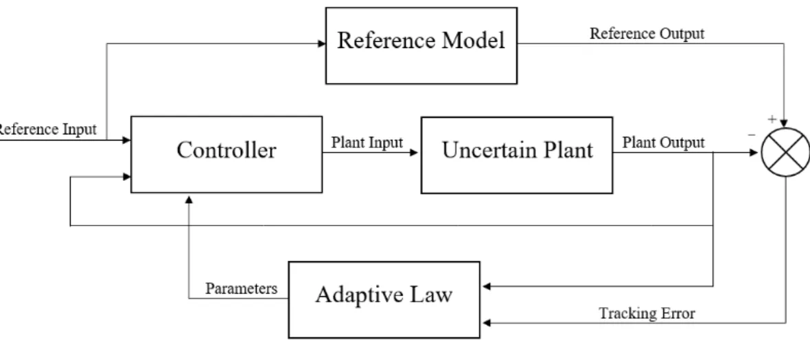
(4.10)

one can apply the Butcher’s algorithm with time step equal to 0.01s generating data to simulate the plant’s behavior, where only the pitch angle perturbation is analyzed:

  

0

0 0 1



 

0 u

w

q



 

 

=



+

 

 

(4.11)

The time step indicated during 120s generates a matrix in Microsoft® Excel® of 12000 rows (from k=0 to k=11999) and 3 columns (t, η, θ) which is important for the adaptive algorithm.

(45)

4.3.2 Lateral-Directional Motion

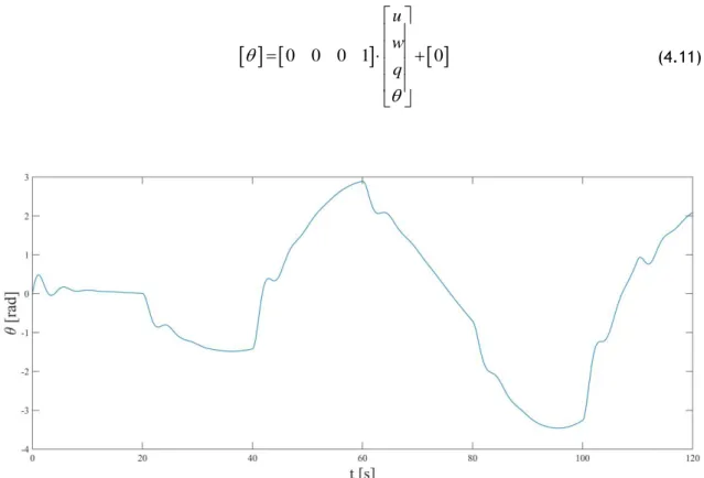
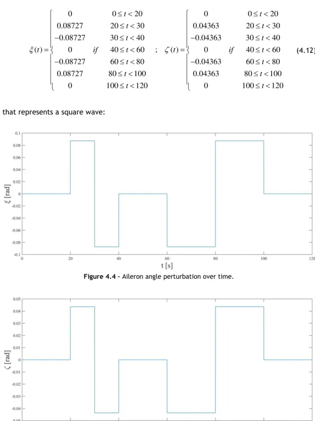
Using (4.2) with the following variations in ξ and ζ over time:

0

20

0

20 0.08727

20

30 0.04363

20

30 0.08727

30

40 0.04363

30

40 ( )

0

40

60 ;

( )

0

40

60 0.08727

60

80 0.04363

60

80 0.08727

80

100 0.04363

80

100

0

100

120

0

100

120 t

t

if

t

if

t





 





_{ }



_{ }



−

 



−

 



=

_

 

=

_

 

−

 

−

 



 



_{ }







(4.12)

that represents a square wave:

Figure 4.4 – Aileron angle perturbation over time.

(46)

and the following initial conditions:

1

0 (0)

0

0 x

 

 

=

 

 

(4.13)

one can apply the Butcher’s algorithm with time step equal to 0.01s generating data to simulate the plant’s behavior, where only the lateral velocity and roll angle perturbations are analyzed:

1

0

1

0

v

p

N

v

r

N

_





 

 

   

  

₌

_{  }

_

+ 



  

_{  }

  







 

 

(4.14)

In order to obtain a more realistic set of data, the output data was corrupted with sensor noise [8], which is usually electrical [12]. Nv is 20% and Nφ is 1% of a Gaussian distribution with

0 mean and variance 1, which according to the original data set, allow to obtain graphics with slightly noise:

(47)

The time step indicated during 120s generates a matrix in Microsoft® Excel® of 12000 rows (from k=0 to k=11999) and several columns which is important for the adaptive algorithm.

4.4 Modeling with System Identification

Linearized equations have been successfully and extensively used in stability and control analysis and also in system identification. System identification is a methodology for determining mathematical models of dynamic systems using measurement observations of the system’s inputs and outputs [52], [53].

In this section, the previously generated data set in combination with the adaptation mechanism from section 3.1 are used to build mathematical models of the F-4C aircraft. The system identification process is represented schematically, where the airplane behaves well as a 3rd_{order system (n=3) for both motion cases and flight conditions. The goal of the}

scheme represented in Figure 4.8 is to obtain a vector of estimation parameters, in which the best estimation corresponds to k=11999. This vector will be used to translate the aircraft behavior in the model. It is important to know that any model is only an approximation of the actual plant, which can only reproduce some plant properties in such a way that some control design is possible [55].

The time delay of the adaptation algorithm was set as equal to 1. In order to prevent

0

ˆ ( ) 0

b k

→

,

d

ˆ ( ) 0

₀

k

→

and gˆ ( )₀ k →0, the initial values of the estimation parameter vector were set as



1 0 0 0 0 0



for the longitudinal case and



1 0 0 0 0 0 0 0 0



for the lateral-directional case. These conditions are also valid for the controller simulation section.

(48)

For the longitudinal motion, this scheme is applied using up(t): η(t) and yp(t): θ(t) to obtain the

system model

y

_p

( )

k

=

p

ˆ

T

(11999)

  −

(

k

1)

. For the lateral-directional motion, the scheme is applied using up(t): ξ(t); ζ(t) and yp(t): φnoise(t); vnoise(t) to obtain the system models

(1)

_ˆ

(1) (1)

( )

T

(11999)

(

1)

p

y

k

=

p

 

k

−

and

y

(2)_p

( )

k

=

p

ˆ

(2)T

(11999)

 

(2)

(

k

−

1)

that must be used simultaneously in the algorithm.

(49)

Chapter 5 – Controller Simulation:

Results and Discussion

5.1 Simulation Conditions

The system models for the two cases are then used in the MRAC algorithm to behave like an approximation of the real F-4C Phantom, where the correct choice of the initial simulation conditions is essential for the precise operation of the controller. In the full algorithm, the estimation parameter vectors are updated in real-time so that the adaptive control can adjust the control law in order to track the reference output (yref) with acceptable stability.

Figure 5.1 describes schematically the full MRAC simulation algorithm, where yref is a set of

generated reference data to test the controller.

This scheme is based on the work from [13] and is applied on both simulation cases.

Sometimes when dealing with real aircraft, the implementation of an adaptive control design can be difficult because of actuator magnitude and rate saturation. Such limitations can lead to incorrect learning of the adaptive mechanism during periods of saturation [8]. In the present study, the simulation conditions were controlled to avoid a non-linear problem, since it is not the main focus of this dissertation.

Aircraft Attitude Tracking using a Model Reference Adaptive Control

UNIVERSIDADE DA BEIRA INTERIOR

Engenharia