A Genetic Algorithm Tutorial
Darrell Whitley
Computer Science Department, Colorado State University
Fort Collins, CO 80523
[email protected]
Abstract
This tutorial covers the canonical genetic algorithm as well as more experimental forms of genetic algorithms, including parallel island models and parallel cellular genetic algorithms. The tutorial also illustrates genetic search by hyperplane sampling. The theoretical foundations of genetic algorithms are reviewed, include the schema theorem as well as recently developed exact models of the canonical genetic algorithm.
Keywords: Genetic Algorithms, Search, Parallel Algorithms
1 Introduction
Genetic Algorithms are a family of computational models inspired by evolution. These
algorithms encode a potential solution to a specic problem on a simple chromosome-like data structure and apply recombination operators to these structures so as to preserve critical information. Genetic algorithms are often viewed as function optimizers, although the range of problems to which genetic algorithms have been applied is quite broad.
An implementation of a genetic algorithm begins with a population of (typically random) chromosomes. One then evaluates these structures and allocates reproductive opportunities in such a way that those chromosomeswhich represent a better solution to the target problem are given more chances to \reproduce" than those chromosomes which are poorer solutions. The \goodness" of a solution is typically dened with respect to the current population.
This particular description of a genetic algorithm is intentionally abstract because in some sense, the term genetic algorithm has two meanings. In a strict interpretation, the
genetic algorithm refers to a model introduced and investigated by John Holland (1975) and
by students of Holland (e.g., DeJong, 1975). It is still the case that most of the existing theory for genetic algorithms applies either solely or primarily to the model introduced by Holland, as well as variations on what will be referred to in this paper as the canonical
genetic algorithm. Recent theoretical advances in modeling genetic algorithms also apply
primarily to the canonical genetic algorithm (Vose, 1993).
In a broader usage of the term, a genetic algorithm is any population-based model that uses selection and recombination operators to generate new sample points in a search space. Many genetic algorithm models have been introduced by researchers largely working from
an experimental perspective. Many of these researchers are application oriented and are typically interested in genetic algorithms as optimization tools.
The goal of this tutorial is to present genetic algorithms in such a way that students new to this eld can grasp the basic concepts behind genetic algorithms as they work through the tutorial. It should allow the more sophisticated reader to absorb this material with relative ease. The tutorial also covers topics, such as inversion, which have sometimes been misunderstood and misused by researchers new to the eld.
The tutorial begins with a very low leveldiscussion of optimizationto both introduce basic ideas in optimization as well as basic concepts that relate to genetic algorithms. In section 2 a canonical genetic algorithm is reviewed. In section 3 the principle of hyperplane sampling is explored and some basic crossover operators are introduced. In section 4 various versions of the schema theorem are developed in a step by step fashion and other crossover operators are discussed. In section 5 binary alphabets and their eects on hyperplane sampling are considered. In section 6 a brief criticism of the schema theorem is considered and in section 7 an exact model of the genetic algorithm is developed. The last three sections of the tutorial cover alternativeforms of genetic algorithms and evolutionary computational models, including specialized parallel implementations.
1.1 Encodings and Optimization Problems
Usually there are only two main components of most genetic algorithms that are problem dependent: the problem encoding and the evaluation function.
Consider a parameter optimization problem where we must optimize a set of variables ei-ther to maximizesome target such as prot, or to minimizecost or some measure of error. We might view such a problem as a black box with a series of control dials representing dierent parameters the only output of the black box is a value returned by an evaluation function indicating how well a particular combination of parameter settings solves the optimization problem. The goal is to set the various parameters so as to optimize some output. In more traditional terms, we wish to minimize (or maximize) some function F(X
1 X
2 :::X
M).
Most users of genetic algorithms typically are concerned with problems that are nonlinear. This also often implies that it is not possible to treat each parameter as an independent variable which can be solved in isolation from the other variables. There are interactions such that the combined eects of the parameters must be considered in order to maximize or minimize the output of the black box. In the genetic algorithm community, the interaction between variables is sometimes referred to as epistasis.
The rst assumption that is typically made is that the variables representing parameters can be represented by bit strings. This means that the variables are discretized in an a priori fashion, and that the range of the discretization corresponds to some power of 2. For example, with 10 bits per parameter, we obtain a range with 1024 discrete values. If the parameters are actually continuous then this discretization is not a particular problem. This assumes, of course, that the discretization provides enough resolution to make it possible to adjust the output with the desired level of precision. It also assumes that the discretization is in some sense representative of the underlying function.
If some parameter can only take on an exact nite set of values then the coding issue becomes more dicult. For example, what if there are exactly 1200 discrete values which can be assigned to some variable X
i. We need at least 11 bits to cover this range, but
this codes for a total of 2048 discrete values. The 848 unnecessary bit patterns may result in no evaluation, a default worst possible evaluation, or some parameter settings may be represented twice so that all binary strings result in a legal set of parameter values. Solving such coding problems is usually considered to be part of the design of the evaluation function. Aside from the coding issue, the evaluation function is usually given as part of the problem description. On the other hand, developing an evaluation function can sometimes involve developing a simulation. In other cases, the evaluation may be performance based and may represent only an approximate or partial evaluation. For example, consider a control application where the system can be in any one of an exponentially large number of possible states. Assume a genetic algorithm is used to optimize some form of control strategy. In such cases, the state space must be sampled in a limited fashion and the resulting evaluation of control strategies is approximate and noisy (c.f., Fitzpatrick and Grefenstette, 1988).
The evaluation function must also be relatively fast. This is typically true for any opti-mization method, but it may particularly pose an issue for genetic algorithms. Since a genetic algorithm works with a population of potential solutions, it incurs the cost of evaluating this population. Furthermore, the population is replaced (all or in part) on a generational basis. The members of the population reproduce, and their ospring must then be evaluated. If it takes 1 hour to do an evaluation, then it takes over 1 year to do 10,000 evaluations. This would be approximately 50 generations for a population of only 200 strings.
1.2 How Hard is Hard?
Assuming the interaction between parameters is nonlinear, the size of the search space is related to the number of bits used in the problem encoding. For a bit string encoding of length L the size of the search space is 2
L and forms a hypercube. The genetic algorithm
samples the corners of this L-dimensional hypercube.
Generally, most test functions are at least 30 bits in length and most researchers would probably agree that larger test functions are needed. Anything much smaller represents a space which can be enumerated. (Considering for a moment that the national debt of the United States in 1993 is approximately 242 dollars, 230 does not sound quite so large.) Of
course, the expression 2L grows exponentially with respect to
L. Consider a problem with
an encoding of 400 bits. How big is the associated search space? A classic introductory textbook on Articial Intelligence gives one characterization of a space of this size. Winston (1992:102) points out that 2400is a good approximation of the eective size of the search space
of possible board congurations in chess. (This assumes the eective branching factor at each possible move to be 16 and that a game is made up of 100 moves 16100 = (24)100 = 2400).
Winston states that this is \a ridiculously large number. In fact, if all the atoms in the universe had been computing chess moves at picosecond rates since the big bang (if any), the analysis would be just getting started."
The point is that as long as the number of \good solutions" to a problem are sparse with respect to the size of the search space, then random search or search by enumeration of a large
search space is not a practical form of problem solving. On the other hand, any search other than random search imposes some bias in terms of how it looks for better solutions and where it looks in the search space. Genetic algorithms indeed introduce a particular bias in terms of what new points in the space will be sampled. Nevertheless, a genetic algorithm belongs to the class of methods known as \weak methods" in the Articial Intelligence community because it makes relatively few assumptions about the problem that is being solved.
Of course, there are many optimization methods that have been developed in mathe-matics and operations research. What role do genetic algorithms play as an optimization tool? Genetic algorithms are often described as a global search method that does not use gradient information. Thus, nondierentiable functions as well as functions with multiple local optima represent classes of problems to which genetic algorithms might be applied. Genetic algorithms, as a weak method, are robust but very general. If there exists a good specialized optimization method for a specic problem, then genetic algorithm may not be the best optimization tool for that application. On the other hand, some researchers work with hybrid algorithms that combine existing methods with genetic algorithms.
2 The Canonical Genetic Algorithm
The rst step in the implementation of any genetic algorithm is to generate an initial pop-ulation. In the canonical genetic algorithm each member of this population will be a binary string of length L which corresponds to the problem encoding. Each string is sometimes referred to as a \genotype" (Holland, 1975) or, alternatively, a \chromosome" (Schaer, 1987). In most cases the initial population is generated randomly. After creating an initial population, each string is then evaluated and assigned a tness value.
The notion of evaluation and tness are sometimes used interchangeably. However, it is useful to distinguish between the evaluation function and the tness function used by a genetic algorithm. In this tutorial, the evaluation function, or objective function, provides a measure of performance with respect to a particular set of parameters. Thetness function
transforms that measure of performance into an allocation of reproductive opportunities. The evaluation of a string representing a set of parameters is independent of the evaluation of any other string. The tness of that string, however, is always dened with respect to other members of the current population.
In the canonical genetic algorithm, tness is dened by: f i
=fwhere f
i is the evaluation
associated with string i and f is the average evaluation of all the strings in the population.
Fitness can also be assigned based on a string's rank in the population (Baker, 1985 Whitley, 1989) or by sampling methods, such as tournament selection (Goldberg, 1990).
It is helpful to view the execution of the genetic algorithm as a two stage process. It starts with thecurrent population. Selection is applied to the current population to create an
intermediate population. Then recombination and mutation are applied to the intermediate
population to create the next population. The process of going from the current population to the next population constitutes one generation in the execution of a genetic algorithm. Goldberg (1989) refers to this basic implementation as a Simple Genetic Algorithm (SGA).
String 1
String 2
String 3
String 4
String 1
String 2
String 2
String 4
(Duplication) (Crossover)
Next
Generation t + 1 Intermediate
Generation t Generation t
Current
Selection Recombination
Offspring-A (1 X 2)
Offspring-B (1 X 2)
Offspring-A (2 X 4)
Offspring-B (2 X 4)
Figure 1: One generation is broken down into a selection phase and recombination phase. This gure shows strings being assigned into adjacent slots during selection. In fact, they can be assigned slots randomly in order to shue the intermediate population. Mutation (not shown) can be applied after crossover.
We will rst consider the construction of the intermediate population from the current population. In the rst generation the current population is also the initial population. After calculating f
i
=ffor all the strings in the current population, selection is carried out. In the
canonical genetic algorithm the probability that strings in the current population are copied (i.e., duplicated) and placed in the intermediate generation is proportion to their tness.
There are a number of ways to do selection. We might view the population as mapping onto a roulette wheel, where each individual is represented by a space that proportionally corresponds to its tness. By repeatedly spinning the roulette wheel, individuals are chosen using \stochastic sampling with replacement" to ll the intermediate population.
A selection process that will more closely match the expected tness values is \remainder stochastic sampling." For each stringi wheref
i
=fis greater than 1.0, the integer portion of
this number indicates how many copies of that string are directly placed in the intermediate population. All strings (including those withf
i
=fless than 1.0) then place additional copies
in the intermediate population with a probability corresponding to the fractional portion of
f i
=f. For example, a string with f i
=f= 1:36 places 1 copy in the intermediate population,
and then receivesa 0:36 chance of placing a second copy. A string with a tness off i
=f= 0:54
has a 0:54 chance of placing one string in the intermediate population.
\Remainder stochastic sampling" is most eciently implemented using a method known
as Stochastic Universal Sampling. Assume that the population is laid out in random order
as in a pie graph, where each individual is assigned space on the pie graph in proportion to tness. Next an outer roulette wheel is placed around the pie with N equally spaced pointers. A single spin of the roulette wheel will now simultaneously pick all N members of the intermediate population. The resulting selection is also unbiased (Baker, 1987).
After selection has been carried out the construction of the intermediate population is complete and recombination can occur. This can be viewed as creating the next population
from the intermediate population. Crossover is applied to randomly paired strings with a probability denoted pc. (The population should already be suciently shued by the
random selection process.) Pick a pair of strings. With probability pc \recombine" these
strings to form two new strings that are inserted into the next population.
Consider the following binary string: 1101001100101101. The string would represent a possible solution to some parameter optimization problem. New sample points in the space are generated by recombining two parent strings. Consider the string 1101001100101101 and another binary string, yxyyxyxxyyyxyxxy, in which the values 0 and 1 are denoted by x and y. Using a single randomly chosen recombination point, 1-point crossover occurs as follows.
11010 \/ 01100101101 yxyyx /\ yxxyyyxyxxy
Swapping the fragments between the two parents produces the following ospring.
11010yxxyyyxyxxy and yxyyx01100101101
After recombination, we can apply a mutation operator. For each bit in the population, mutate with some low probabilitypm. Typically the mutation rate is applied with less than
1% probability. In some cases, mutation is interpreted as randomly generating a new bit, in which case, only 50% of the time will the \mutation" actually change the bit value. In other cases, mutation is interpreted to mean actually ipping the bit. The dierence is no more than an implementation detail as long as the user/reader is aware of the dierence and understands that the rst form of mutation produces a change in bit values only half as often as the second, and that one version of mutation is just a scaled version of the other.
After the process of selection, recombination and mutation is complete, the next popu-lation can be evaluated. The process of evaluation, selection, recombination and mutation forms one generation in the execution of a genetic algorithm.
2.1 Why does it work? Search Spaces as Hypercubes.
The question that most people who are new to the eld of genetic algorithms ask at this point is why such a process should do anything useful. Why should one believe that this is going to result in an eective form of search or optimization?
The answer which is most widely given to explain the computational behavior of genetic algorithms came out of John Holland's work. In his classic 1975 book, Adaptation in
Nat-ural and Articial Systems, Holland develops several arguments designed to explain how a
\genetic plan" or \genetic algorithm" can result in complex and robust search by implicitly sampling hyperplane partitions of a search space.
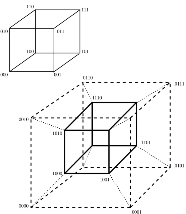
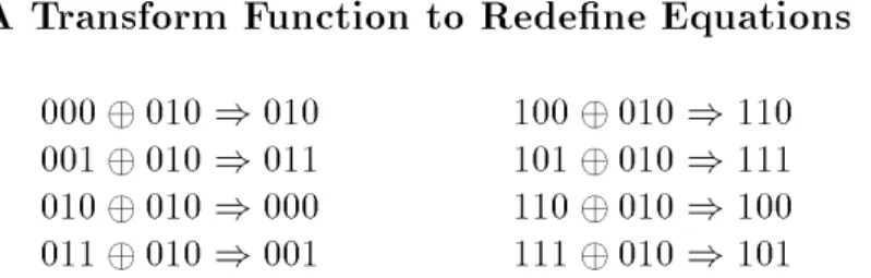
Perhaps the best way to understand how a genetic algorithm can sample hyperplane partitions is to consider a simple 3-dimensional space (see Figure 2). Assume we have a problem encoded with just 3 bits this can be represented as a simple cube with the string 000 at the origin. The corners in this cube are numbered by bit strings and all adjacent corners are labelled by bit strings that dier by exactly 1-bit. An example is given in the top of Figure 2. The front plane of the cube contains all the points that begin with 0. If \*" is used as a \don't care" or wild card match symbol, then this plane can also be represented by the special string 0**. Strings that contain *are referred to as schemata each schema corresponds to a hyperplane in the search space. The \order" of a hyperplane refers to the number of actual bit values that appear in its schema. Thus, 1** is order-1 while 1**1******0** would be of order-3.
The bottom of Figure 2 illustrates a 4-dimensional space represented by a cube \hanging" inside another cube. The points can be labeled as follows. Label the points in the inner cube and outer cube exactly as they are labeled in the top 3-dimensional space. Next, prex each inner cube labeling with a 1 bit and each outer cube labeling with a 0 bit. This creates an assignment to the points in hyperspace that gives the proper adjacency in the space between strings that are 1 bit dierent. The inner cube now corresponds to the hyperplane 1*** while the outer cube corresponds to 0***. It is also rather easy to see that *0** corresponds to the subset of points that corresponds to the fronts of both cubes. The order-2 hyperplane 10** corresponds to the front of the inner cube.
A bit string matches a particular schemata if that bit string can be constructed from the schemata by replacing the \*" symbol with the appropriate bit value. In general, all bit strings that match a particular schemata are contained in the hyperplane partition rep-resented by that particular schemata. Every binary encoding is a \chromosome" which corresponds to a corner in the hypercube and is a member of 2L
;1 dierent hyperplanes,
where L is the length of the binary encoding. (The string of all *symbols corresponds to
the space itself and is not counted as a partition of the space (Holland 1975:72)). This can be shown by taking a bit string and looking at all the possible ways that any subset of bits can be replaced by \*" symbols. In other words, there are L positions in the bit string and
each position can be either the bit value contained in the string or the \*" symbol. It is also relatively easy to see that 3L
;1 hyperplane partitions can be dened over the
entire search space. For each of theLpositions in the bit string we can have either the value
*, 1 or 0 which results in 3L combinations.
Establishing that each string is a member of 2L
;1 hyperplane partitions doesn't provide
very much information if each point in the search space is examined in isolation. This is why the notion of a population based search is critical to genetic algorithms. A population of sample points provides information about numerous hyperplanes furthermore, low order hyperplanes should be sampled by numerous points in the population. (This issue is reexam-ined in more detail in subsequent sections of this paper.) A key part of a genetic algorithm's
intrinsic or implicit parallelismis derived from the fact that many hyperplanes are sampled
when a population of strings is evaluated (Holland 1975) in fact, it can be argued that far more hyperplanes are sampled than the number of strings contained in the population. Many
010
000
110
001 011
100
111
101
0001
0101 0111
0000 0010
1000
1101 1010
1110
1001 0110
Figure 2: A 3-dimensional cube and a 4-dimensional hypercube. The corners of the inner
cube and outer cube in the bottom 4-D example are numbered in the same way as in the upper 3-D cube, except a 1 is added as a prex to the labels of inner cube and a 0 is added as a prex to the labels of the outer cube. Only select points are labeled in the 4-D hypercube.
dierent hyperplanes are evaluated in an implicitly parallel fashion each time a single string is evaluated (Holland 1975:74) but it is the cumulative eects of evaluating a population of points that provides statistical information about any particular subset of hyperplanes.1
Implicit parallelismimplies that many hyperplane competitions are simultaneously solved
in parallel. The theory suggests that through the process of reproduction and recombination, the schemata of competing hyperplanes increase or decrease their representation in the pop-ulation according to the relative tness of the strings that lie in those hyperplane partitions. Because genetic algorithms operate on populations of strings, one can track the proportional representation of a single schema representing a particular hyperplane in a population and indicate whether that hyperplane will increase or decrease its representation in the popula-tion over time when tness based selecpopula-tion is combined with crossover to produce ospring from existing strings in the population.
3 Two Views of Hyperplane Sampling
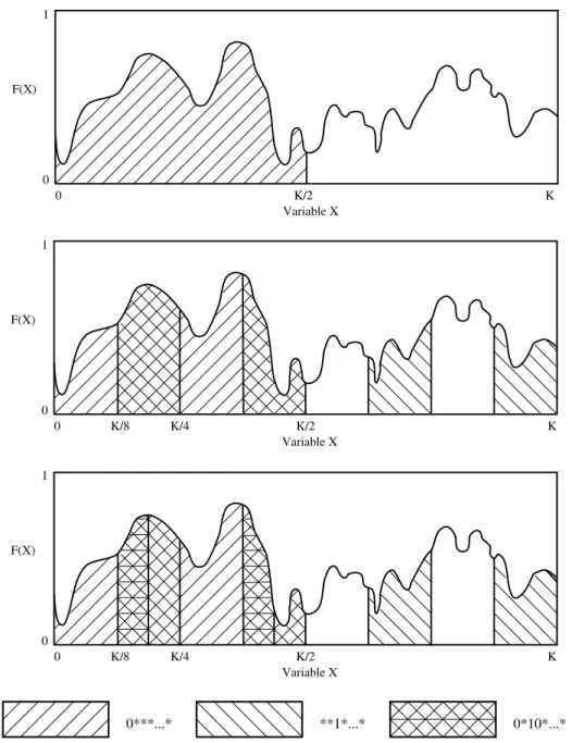
Another way of looking at hyperplane partitions is presented in Figure 3. A function over a single variable is plotted as a one-dimensional space, with function maximization as a goal. The hyperplane 0****...** spans the rst half of the space and 1****...** spans the second half of the space. Since the strings in the 0****...** partition are on average better than those in the 1****...** partition, we would like the search to be proportionally biased toward this partition. In the second graph the portion of the space corresponding to **1**...** is shaded, which also highlights the intersection of 0****...** and **1**...**, namely, 0*1*...**. Finally, in the third graph, 0*10**...** is highlighted.
One of the points of Figure 3 is that the sampling of hyperplane partitions is not really eected by local optima. At the same time, increasing the sampling rate of partitions that are above average compared to other competing partitions does not guarantee convergence to a global optimum. The global optimum could be a relatively isolated peak, for example. Nevertheless, good solutions that are globally competitive should be found.
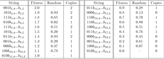
It is also a useful exercise to look at an example of a simple genetic algorithm in action. In Table 1, the rst 3 bits of each string are given explicitly while the remainder of the bit positions are unspecied. The goal is to look at only those hyperplanes dened over the rst 3 bit positions in order to see what actually happens during the selection phase when strings are duplicated according to tness. The theory behind genetic algorithms suggests that the new distribution of points in each hyperplane should change according to the average tness of the strings in the population that are contained in the corresponding hyperplane partition. Thus, even though a genetic algorithm never explicitly evaluates any particular hyperplane partition, it should change the distribution of string copies as if it had.
1Holland initially used the term intrinsic parallelismin his 1975 monograph, then decided to switch to
implicit parallelism to avoid confusion with terminology in parallel computing. Unfortunately, the term
implicit parallelismin the parallel computing community refers to parallelism which is extracted from code written in functional languages that have no explicit parallel constructs. Implicit parallelismdoes not refer to the potential for running genetic algorithms on parallel hardware, although genetic algorithms are generally viewed as highly parallelizable algorithms.
F(X)
0 K/2 K Variable X
0 1
0 K/8 K/4 K/2 K Variable X
0 1
F(X)
0 K/8 K/4 K/2 K Variable X
0 1
F(X)
0***...* **1*...* 0*10*...*
Figure 3: A function and various partitions of hyperspace. Fitness is scaled to a 0 to 1 range in this diagram.
String Fitness Random Copies String Fitness Random Copies 001b
14... b
1L 2.0 { 2 011
b 124...
b
12L 0.9 0.28 1
101b 24...
b
2L 1.9 0.93 2 000
b 134...
b
13L 0.8 0.13 0
111b 34...
b
3L 1.8 0.65 2 110
b 144...
b
14L 0.7 0.70 1
010b 44...
b
4L 1.7 0.02 1 110
b 154...
b
15L 0.6 0.80 1
111b 54...
b
5L 1.6 0.51 2 100
b 164...
b
16L 0.5 0.51 1
101b 64...
b
6L 1.5 0.20 1 011
b 174...
b
17L 0.4 0.76 1
011b 74...
b
7L 1.4 0.93 2 000
b 184...
b
18L 0.3 0.45 0
001b 84...
b
8L 1.3 0.20 1 001
b 194...
b
19L 0.2 0.61 0
000b 94...
b
9L 1.2 0.37 1 100
b 204...
b
20L 0.1 0.07 0
100b 104...
b
10L 1.1 0.79 1 010
b 214...
b
21L 0.0 { 0
010b 114...
b
11L 1.0 { 1
Table 1: A population with tness assigned to strings according to rank.
Random
is a random number which determines whether or not a copy of a string is awarded for the fractional remainder of the tness.The example population in Table 1 contains only 21 (partially specied) strings. Since we are not particularly concerned with the exact evaluation of these strings, the tness values will be assigned according to rank. (The notion of assigning tness by rank rather than by tness proportional representation has not been discussed in detail, but the current example relates to change in representation due to tness and not how that tness is assigned.) The table includes information on the tness of each string and the number of copies to be placed in the intermediate population. In this example, the number of copies produced during selection is determined by automatically assigning the integer part, then assigning the fractional part by generating a random value between 0.0 and 1.0 (a form of remainder stochastic sampling). If the random value is greater than (1;remainder) then an additional
copy is awarded to the corresponding individual.
Genetic algorithms appear to process many hyperplanes implicitly in parallel when selec-tion acts on the populaselec-tion. Table 2 enumerates the 27 hyperplanes (33) that can be dened
over the rst three bits of the strings in the population and explicitly calculates the tness associated with the corresponding hyperplane partition. The true tness of the hyperplane partition corresponds to the average tness of all strings that lie in that hyperplane parti-tion. The genetic algorithm uses the population as a sample for estimating the tness of that hyperplane partition. Of course, the only time the sample is random is during the rst generation. After this, the sample of new strings should be biased toward regions that have previously contained strings that were above average with respect to previous populations.
If the genetic algorithm works as advertised, the number of copies of strings that actually fall in a particular hyperplane partition after selection should approximate the expected number of copies that should fall in that partition.
Schemata and Fitness Values
Schema Mean Count Expect Obs Schema Mean Count Expect Obs
101*...* 1.70 2 3.4 3 *0**...* 0.991 11 10.9 9
111*...* 1.70 2 3.4 4 00**...* 0.967 6 5.8 4
1*1*...* 1.70 4 6.8 7 0***...* 0.933 12 11.2 10
*01*...* 1.38 5 6.9 6 011*...* 0.900 3 2.7 4
**1*...* 1.30 10 13.0 14 010*...* 0.900 3 2.7 2
*11*...* 1.22 5 6.1 8 01**...* 0.900 6 5.4 6
11**...* 1.175 4 4.7 6 0*0*...* 0.833 6 5.0 3
001*...* 1.166 3 3.5 3 *10*...* 0.800 5 4.0 4
1***...* 1.089 9 9.8 11 000*...* 0.767 3 2.3 1
0*1*...* 1.033 6 6.2 7 **0*...* 0.727 11 8.0 7
10**...* 1.020 5 5.1 5 *00*...* 0.667 6 4.0 3
*1**...* 1.010 10 10.1 12 110*...* 0.650 2 1.3 2
****...* 1.000 21 21.0 21 1*0*...* 0.600 5 3.0 4
100*...* 0.566 3 1.70 2
Table 2: The average tnesses (Mean) associated with the samples from the 27 hyperplanes dened over the rst three bit positions are explicitly calculated. The Expected representation (Expect) and Observed representation (Obs) are shown. Count refers to the number of strings in hyperplane H before selection.
In Table 2, theexpectednumber of strings sampling a hyperplane partition after selection can be calculated by multiplying the number of hyperplane samples in the current population before selection by the average tness of the strings in the population that fall in that partition. The observed number of copies actually allocated by selection is also given. In most cases the match between expected and observed sampling rate is fairly good: the error is a result of sampling error due to the small population size.
It is useful to begin formalizing the idea of tracking the potential sampling rate of a hyperplane, H. LetM(Ht) be the number of strings sampling H at the current generation t in some population. Let (t+intermediate) index the generation t after selection (but before crossover and mutation), and f(Ht) be the average evaluation of the sample of strings in partition H in the current population. Formally, the change in representation according to tness associated with the strings that are drawn from hyperplane H is expressed by:
M(Ht + intermediate) = M(Ht)f(Ht)f :
Of course, when strings are merely duplicated no new sampling of hyperplanes is actu-ally occurring since no new samples are generated. Theoreticactu-ally, we would like to have a sample of new points with this same distribution. In practice, this is generally not possible. Recombination and mutation, however, provides a means of generating new sample points while partially preserving distribution of strings across hyperplanes that is observed in the intermediate population.
3.1 Crossover Operators and Schemata
The observed representation of hyperplanes in Table 2 corresponds to the representation in
the intermediate population after selection but before recombination. What does recombi-nation do to the observed string distributions? Clearly, order-1 hyperplane samples are not aected by recombination, since the single critical bit is always inherited by one of the o-spring. However, the observed distribution of potential samples from hyperplane partitions of order-2 and higher can be aected by crossover. Furthermore, all hyperplanes of the same order are not necessarily aected with the same probability. Consider 1-point crossover. This recombination operator is nice because it is relatively easy to quantify its eects on dierent schemata representing hyperplanes. To keep things simple, assume we are are working with a string encoded with just 12 bits. Now consider the following two schemata.
11********** and 1**********1
The probability that the bits in the rst schema will be separated during 1-point crossover is only 1=L;1, since in general there are L;1 crossover points in a string of length L. The
probability that the bits in the second rightmost schema are disrupted by 1-point crossover however is (L;1)=(L;1), or 1.0, since each of the L-1 crossover points separates the bits in
the schema. This leads to a general observation: when using 1-point crossover the positions of the bits in the schema are important in determining the likelihood that those bits will remain together during crossover.
3.1.1 2-point Crossover
What happens if a 2-point crossover operator is used? A 2-point crossover operator uses two randomly chosen crossover points. Strings exchange the segment that falls between these two points. Ken DeJong rst observed (1975) that 2-point crossover treats strings and schemata as if they form a ring, which can be illustrated as follows:
b7 b6 b5 * * *
b8 b4 * *
b9 b3 * *
b10 b2 * *
b11 b12 b1 * 1 1
where b1 to b12 represents bits 1 to 12. When viewed in this way, 1-point crossover
is a special case of 2-point crossover where one of the crossover points always occurs at the wrap-around position between the rst and last bit. Maximum disruptions for order-2 schemata now occur when the 2 bits are at complementary positions on this ring.
For 1-point and 2-point crossover it is clear that schemata which have bits that are close together on the string encoding (or ring) are less likely to be disrupted by crossover. More precisely, hyperplanes represented by schemata with more compact representations should be sampled at rates that are closer to those potential sampling distribution targets achieved under selection alone. For current purposes a compact representation with respect
to schemata is one that minimizes the probability of disruption during crossover. Note that this denition is operator dependent, since both of the two order-2 schemata examined in section 3.1 are equally and maximally compact with respect to 2-point crossover, but are maximally dierent with respect to 1-point crossover.
3.1.2 Linkage and Dening Length
Linkage refers to the phenomenon whereby a set of bits act as \coadapted alleles" that tend
to be inherited together as a group. In this case an allele would correspond to a particular bit value in a specic position on the chromosome. Of course, linkage can be seen as a generalization of the notion of a compact representation with respect to schema. Linkage is is sometimed dened by physical adjacency of bits in a string encoding this implicitly assumes that 1-point crossover is the operator being used. Linkage under 2-point crossover is dierent and must be dened with respect to distance on the chromosome when treated as a ring. Nevertheless, linkage usually is equated with physical adjacency on a string, as measured by dening length.
Thedening lengthof a schemata is based on the distance between the rst and last bits
in the schema with value either 0 or 1 (i.e., not a *symbol). Given that each position in a schema can be 0, 1 or *, then scanning left to right, if I
x is the index of the position of
the rightmost occurrence of either a 0 or 1 and I
y is the index of the leftmost occurrence
of either a 0 or 1, then the dening length is merely I x
;I y
: Thus, the dening length of
****1**0**10** is 12;5 = 7. The dening length of a schema representing a hyperplane H is denoted here by "(H). The dening length is a direct measure of how many possible
crossover points fall within the signicant portion of a schemata. If 1-point crossover is used, then "(H)=L;1 is also a direct measure of how likely crossover is to fall within the
signicant portion of a schemata during crossover.
3.1.3 Linkage and Inversion
Along with mutation and crossover,inversionis often considered to be a basic genetic oper-ator. Inversion can change the linkage of bits on the chromosome such that bits with greater nonlinear interactions can potentially be moved closer together on the chromosome.
Typically, inversion is implemented by reversing a random segment of the chromosome. However, before one can start moving bits around on the chromosome to improve linkage, the bits must have a position independent decoding. A common error that some researchers make when rst implementing inversion is to reverse bit segments of a directly encoded chromosome. But just reversing some random segment of bits is nothing more than large scale mutation if the mapping from bits to parameters is position dependent.
A position independent encoding requires that each bit be tagged in some way. For example, consider the following encoding composed of pairs where the rst number is a bit tag which indexes the bit and the second represents the bit value.
((9 0) (6 0) (2 1) (7 1) (5 1) (8 1) (3 0) (1 0) (4 0))
The linkage can now be changed by moving around the tag-bit pairs, but the string remains the same when decoded: 010010110. One must now also consider how recombination is to be implemented. Goldberg and Bridges (1990), Whitley (1991) as well as Holland (1975) discuss the problems of exploiting linkage and the recombination of tagged representations.
4 The Schema Theorem
A foundation has been laid to now develop the fundamental theorem of genetic algorithms.
The schema theorem(Holland, 1975) provides a lower bound on the change in the sampling
rate for a single hyperplane from generation t to generation t + 1.
Consider again what happens to a particular hyperplane,H when only selection occurs. M(Ht + intermediate) = M(Ht)f(Ht)f :
To calculate M(H,t+1) we must consider the eects of crossover as the next generation is created from the intermediate generation. First we consider that crossover is applied probabilistically to a portion of the population. For that part of the population that does not undergo crossover, the representation due to selection is unchanged. When crossover does occur, then we must calculate losses due to its disruptive eects.
M(Ht + 1) = (1;p
c)M(Ht)f(Ht)f + pc "
M(Ht)f(Ht)f (1;losses) + gains #
In the derivation of the schema theorem a conservative assumption is made at this point. It is assumed that crossover within the dening length of the schema is always disruptive to the schema representing H. In fact, this is not true and an exact calculation of the eects of crossover is presented later in this paper. For example, assume we are interested in the schema 11*****. If a string such as 1110101 were recombined between the rst two bits with a string such as 1000000 or 0100000, no disruption would occur in hyperplane 11***** since one of the ospring would still reside in this partition. Also, if 1000000 and 0100000 were recombined exactly between the rst and second bit, a new independent ospring would sample 11***** this is the sources of gains that is referred to in the above calculation. To simplify things, gains are ignored and the conservative assumption is made that crossover falling in the signicant portion of a schema always leads to disruption. Thus,
M(Ht + 1)(1;p
c)M(Ht)f(Ht)f + pc "
M(Ht)f(Ht)f (1;disruptions) #
where disruptions overestimates losses. We might wish to consider one exception: if two strings that both sample H are recombined, then no disruption occurs. Let P(Ht) denote the proportional represention of H obtained by dividing M(Ht) by the population size. The probability that a randomly chosen mate samplesH is just P(Ht). Recall that "(H) is the dening length associated with 1-point crossover. Disruption is therefore given by:
"(H) L;1(1
;P(Ht)):
At this point, the inequality can be simplied. Both sides can be divided by the popula-tion size to convert this into an expression for P(H t+ 1), the proportional representation
of H at generation t+ 1: Furthermore, the expression can be rearranged with respect to pc.
P(H t+ 1) P(H t)
f(H t)
f "
1;pc
"(H) L;1(1
;P(H t)) #
We now have a useful version of the schema theorem (although it does not yet consider mutation) but it is not the only version in the literature. For example, both parents are typically chosen based on tness. This can be added to the schema theorem by merely indicating the alternative parent is chosen from the intermediate population after selection.
P(H t+ 1) P(H t)
f(H t)
f "
1;pc
"(H) L;1(1
;P(H t)
f(H t)
f
)
#
Finally, mutation is included. Let o(H) be a function that returns the order of the
hyperplane H. The order of H exactly corresponds to a count of the number of bits in the
schema representing H that have value 0 or 1. Let the mutation probability be pm where
mutation always ips the bit. Thus the probability that mutation does aect the schema representing H is (1;pm)o
(H). This leads to the following expression of the schema theorem.
P(H t+ 1)P(H t)
f(H t)
f "
1;pc
"(H) L;1(1
;P(H t)
f(H t)
f
)
#
(1;pm)
o(H)
4.1 Crossover, Mutation and Premature Convergence
Clearly the schema theorem places the greatest emphasis on the role of crossover and hy-perplane sampling in genetic search. To maximize the preservation of hyhy-perplane samples after selection, the disruptive eects of crossover and mutation should be minimized. This suggests that mutation should perhaps not be used at all, or at least used at very low levels. The motivation for using mutation, then, is to prevent the permanent loss of any partic-ular bit or allele. After several generations it is possible that selection will drive all the bits in some position to a single value: either 0 or 1. If this happens without the genetic algo-rithm converging to a satisfactory solution, then the algoalgo-rithm has prematurely converged.
This may particularly be a problem if one is working with a small population. Without a mutation operator, there is no possibility for reintroducing the missing bit value. Also, if the target function is nonstationary and the tness landscape changes over time (which is cer-tainly the case in real biological systems), then there needs to be some source of continuing genetic diversity. Mutation, therefore acts as a background operator, occasionally changing bit values and allowing alternative alleles (and hyperplane partitions) to be retested.
This particular interpretation of mutation ignores its potential as a hill-climbing mech-anism: from the strict hyperplane sampling point of view imposed by the schema theorem mutation is a necessary evil. But this is perhaps a limited point of view. There are several experimental researchers that point out that genetic search using mutation and no crossover often produces a fairly robust search. And there is little or no theory that has addressed the interactions of hyperplane sampling and hill-climbing in genetic search.
Another problem related to premature convergence is the need forscalingthe population tness. As the average evaluation of the strings in the population increases, the variance in tness decreases in the population. There may be little dierence between the best and worst individual in the population after several generations, and the selective pressure based on tness is correspondingly reduced. This problem can partially be addressed by using some form of tness scaling (Grefenstette, 1986 Goldberg, 1989). In the simplest case, one can subtract the evaluation of the worst string in the population from the evaluations of all strings in the population. One can now compute the average string evaluation as well as tness values using this adjusted evaluation, which will increase the resulting selective pressure. Alternatively, one can use a rank based form of selection.
4.2 How Recombination Moves Through a Hypercube
The nice thing about 1-point crossover is that it is easy to model analytically. But it is also easy to show analytically that if one is interested in minimizing schema disruption, then 2-point crossover is better. But operators that use many crossover points should be avoided because of extreme disruption to schemata. This is again a point of view imposed by a strict interpretation of the schema theorem. On the other hand, disruption may not be the only factor aecting the performance of a genetic algorithm.
4.2.1 Uniform Crossover
The operator that has received the most attention in recent years is uniform crossover. Uniform crossover was studied in some detail by Ackley (1987) and popularized by Syswerda (1989). Uniform crossover works as follows: for each bit position 1 to L, randomly pick each bit from either of the two parent strings. This means that each bit is inherited independently from any other bit and that there is, in fact, no linkage between bits. It also means that uniform crossover is unbiased with respect to dening length. In general the probability of disruption is 1;(1=2)
o(H);1, where o(H) is the order of the schema we are interested in.
(It doesn't matter which ospring inherits the rst critical bit, but all other bits must be inherited by that same ospring. This is also a worst case probability of disruption which assumes no alleles found in the schema of interest are shared by the parents.) Thus, for any order-3 schemata the probability of uniform crossover separating the critical bits is always 1; (1=2)
2 = 0
:75. Consider for a moment a string of 9 bits. The dening length of a
schema must equal 6 before the disruptive probabilities of 1-point crossover match those associated with uniform crossover (6/8 = .75). We can dene 84 dierent order-3 schemata over any particular string of 9 bits (i.e., 9 choose 3). Of these schemata, only 19 of the 84 order-2 schemata have a disruption rate higher than 0.75 under 1-point crossover. Another 15 have exactly the same disruption rate, and 50 of the 84 order-2 schemata have a lower disruption rate. It is relative easy to show that, while uniform crossover is unbiased with respect to dening length, it is also generally more disruptive than 1-point crossover. Spears and DeJong (1991) have shown that uniform crossover is in every case more disruptive than 2-point crossover for order-3 schemata for all dening lengths.
0011 0101 0110 1001 1010 1100
0000 1111
0111 1011 1101 1110
1000 0100
0010 0001
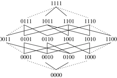
Figure 4: This graph illustrates paths though 4-D space. A 1-point crossover of 1111 and 0000 canonlygenerate ospringthatresidealong the dashedpaths attheedges of thisgraph.
Despite these analytical results, several researchers have suggested that uniform crossover is sometimes a better recombination operator. One can point to its lack of representational bias with respect to schema disruption as a possible explanation, but this is unlikely since uniform crossover is uniformly worse than 2-point crossover. Spears and DeJong (1991:314) speculate that, \With small populations, more disruptive crossover operators such as uniform or n-point (n 2) may yield better results because they help overcome the limited
infor-mation capacity of smaller populations and the tendency for more homogeneity." Eshelman (1991) has made similar arguments outlining the advantages of disruptive operators.
There is another sense in which uniform crossover is unbiased. Assume we wish to recombine the bits string 0000 and 1111. We can conveniently lay out the 4-dimensional hypercube as shown in Figure 4. We can also view these strings as being connected by a set of minimal paths through the hypercube pick one parent string as the origin and the other as the destination. Now change a single bit in the binary representation corresponding to the point of origin. Any such move will reach a point that is one move closer to the destination. In Figure 4 it is easy to see that changing a single bit is a move up or down in the graph.
All of the points between 0000 and 1111 are reachable by some single application of uniform crossover. However, 1-point crossover only generates strings that lie along two com-plementarypaths (in the gure, the leftmost and rightmost paths) through this 4-dimensional hypercube. In general, uniform crossover will draw a complementary pair of sample points with equal probability from all points that lie along any complementary minimal paths in
the hypercube between the two parents, while 1-point crossover samples points from only two specic complementary minimal paths between the two parent strings. It is also easy to see that 2-point crossover is less restrictive than 1-point crossover. Note that the number of bits that are dierent between two strings is just the Hamming distance, H. Not including
the original parent strings, uniform crossover can generate 2H
;2 dierent strings, while
1-point crossover can generate 2(H;1) dierent strings since there are H crossover points
that produce unique ospring (see the discussion in the next section) and each crossover produces 2 ospring. The 2-point crossover operator can generate 2
H 2
=H
2
;H dierent
ospring since there are H choose 2 dierent crossover points that will result in ospring
that are not copies of the parents and each pair of crossover points generates 2 strings.
4.3 Reduced Surrogates
Consider crossing the following two strings and a \reduced" version of the same strings, where the bits the strings share in common have been removed.
0001111011010011 ----11---1---1
0001001010010010 ----00---0---0
Both strings lie in the hyperplane 0001**101*01001*. The ip side of this observation is that crossover is really restricted to a subcube dened over the bit positions that are dierent. We can isolate this subcube by removing all of the bits that are equivalent in the two parent structures. Booker (1987) refers to strings such as ----11---1---1 and ----00---0---0as the \reduced surrogates" of the original parent chromosomes.
When viewed in this way, it is clear that recombinationof these particular strings occurs in a 4-dimensional subcube, more or less identical to the one examined in the previous example. Uniformcrossover is unbiased with respect to this subcube in the sense that uniform crossover will still sample in an unbiased, uniform fashion from all of the pairs of points that lie along complementary minimal paths in the subcube dened between the two original parent strings. On the other hand, simple 1-point or 2-point crossover will not. To help illustrate this idea, we recombine the original strings, but examine the ospring in their \reduced"
forms. For example, simple 1-point crossover will generate ospring ----11---1---0
and ----00---0---1 with a probability of 6/15 since there are 6 crossover points in the
original parent strings between the third and fourth bits in the reduced subcube and L-1 = 15. On the other hand, ----10---0---0 and ----01---1---1 are sampled with a
probability of only 1/15 since there is only a single crossover point in the original parent structures that falls between the rst and second bits that dene the subcube.
One can remove this particular bias, however. We apply crossover on the reduced surro-gates. Crossover can now exploit the fact that there is really only 1 crossover point between any signicant bits that appear in the reduced surrogate forms. There is also another benet. If at least 1 crossover point falls between the rst and last signicant bits in the reduced surrogates, the ospring are guaranteed not to be duplicates of the parents. (This assumes the parents dier by at least two bits). Thus, new sample points in hyperspace are generated. The debate on the merits of uniform crossover and operators such as 2-point reduced sur-rogate crossover is not a closed issue. To fully understand the interaction between hyperplane sampling, population size, premature convergence, crossover operators, genetic diversity and the role of hill-climbing by mutation requires better analytical methods.
5 The Case for Binary Alphabets
The motivation behind the use of a minimal binary alphabet is based on relatively simple counting arguments. A minimal alphabet maximizes the number of hyperplane partitions
rectly available in the encoding for schema processing. These low order hyperplane partitions are also sampled at a higher rate than would occur with an alphabet of higher cardinality.
Any set of order-1 schemata such as 1*** and 0*** cuts the search space in half. Clearly, there are L pairs of order-1 schemata. For order-2 schemata, there are
L 2
ways to pick locations in which to place the 2 critical bits positions, and there are 22 possible ways to
assign values to those bits. In general, if we wish to count how many schemata representing hyperplanes exist at some order i, this value is given by 2
i
L i
where L
i
counts the number of ways to picki positions that will have signicant bit values in a string of length Land 2
i
is the number of ways to assign values to those positions. This ideal can be illustrated for order-1 and order-2 schemata as follows:
Order 1 Schemata Order 2 Schemata
0*** *0** **0* ***0 00** 0*0* 0**0 *00* *0*0 **00
1*** *1** **1* ***1 01** 0*1* 0**1 *01* *0*1 **01
10** 1*0* 1**0 *10* *1*0 **10 11** 1*1* 1**1 *11* *1*1 **11
These counting arguments naturally lead to questions about the relationship between population size and the number of hyperplanes that are sampled by a genetic algorithm. One can take a very simple view of this question and ask how many schemata of order-1 are sampled and how well are they represented in a population of size N. These numbers are based on the assumption that we are interested in hyperplane representations associated with the initial random population, since selection changes the distributions over time. In a population of size N there should be N/2 samples of each of the 2L order-1 hyperplane partitions. Therefore 50% of the population falls in any particular order-1 partition. Each order-2 partition is sampled by 25% of the population. In general then, each hyperplane of order i is sampled by (1=2)
i of the population.
5.1 The
N3
Argument
These counting arguments set the stage for the claim that a genetic algorithm processes on the order ofN
3 hyperplanes when the population size is N. The derivation used here is based
on work found in the appendix of Fitzpatrick and Grefenstette (1988).
Letbe the highest order of hyperplane which is represented in a population of sizeN by
at least copiesis given byl og(N =). We wish to have at least samples of a hyperplane
before claiming that we are statistically sampling that hyperplane.
Recall that the number of dierent hyperplane partitions of order- is given by 2
L
which is just the number of dierent ways to pick dierent positions and to assign all
possible binary values to each subset of the positions. Thus, we now need to show
2
L
!
N
3 which implies 2
L
!
(2
) 3
since = l og(N =) and N = 2
. Fitzpatrick and Grefenstette now make the following
arguments. Assume L 64 and 2 6
N 2
20. Pick
= 8, which implies 3 17: By
inspection the number of schemata processed is greater than N 3.
This argument does not hold in general for any population of size N. Given a string of length L, the number of hyperplanes in the space is nite. However, the population size can be chosen arbitrarily. The total number of schemata associated with a string of length L is 3L. Thus if we pick a population size where
N = 3
L then at most
N hyperplanes can
be processed (Michael Vose, personal communication). Therefore, N must be chosen with
respect to L to make the N
3 argument reasonable. At the same time, the range of values
26
N 2
20 does represent a wide range of practical population sizes.
Still, the argument thatN
3 hyperplanes are usefully processed assumes that all of these
hyperplanes are processed with some degree of independence. Notice that the current deriva-tion counts only those schemata that are exactly of order-. The sum of all schemata from
order-1 to order- that should be well represented in a random initial population is given
by: P x=12
x
L x
. By only counting schemata that are exactly of order- we might hope to
avoid arguments about interactions with lower order schemata. However, all the N
3
argu-ment really shows is that there may be as many asN
3 hyperplanes that are well represented
given an appropriate population size. But a simple static count of the number of schemata available for processing fails to consider the dynamic behavior of the genetic algorithm.
As discussed later in this tutorial, dynamic models of the genetic algorithm now exist (Vose and Liepins, 1991 Whitley, Das and Crabb 1992). There has not yet, however, been any real attempt to use these models to look at complexinteractions between large numbers of hyperplane competitions. It is obvious in some vacuous sense that knowing the distribution of the initial population as well as the tnesses of these strings (and the strings that are subsequently generated by the genetic algorithm) is sucient information for modeling the dynamic behavior of the genetic algorithm (Vose 1993). This suggests that we only need information about those strings sampled by the genetic algorithm. However, this micro-level view of the genetic algorithm does not seems to explain its macro-level processing power.
5.2 The Case for Nonbinary Alphabets
There are two basic arguments against using higher cardinality alphabets. First, there will be fewer explicit hyperplane partitions. Second, the alphabetic characters (and the corresponding hyperplane partitions) associated with a higher cardinality alphabet will not be as well represented in a nite population. This either forces the use of larger population sizes or the eectiveness of statistical sampling is diminished.
The arguments for using binary alphabets assume that the schemata representing hyper-planes must be explicitly and directly manipulated by recombination. Antonisse (1989) has argued that this need not be the case and that higher order alphabets oer as much richness in terms of hyperplane samples as lower order alphabets. For example, using an alphabet of the four characters A, B, C, D one can dene all the same hyperplane partitions in a binary alphabet by dening partitions such as (A and B), (C and D), etc. In general, Antonisse argues that one can look at the all subsets of the power set of schemata as also dening hy-perplanes. Viewed in this way, higher cardinality alphabets yieldmorehyperplane partitions
than binary alphabets. Antonisse's arguments fail to show however, that the hyperplanes that corresponds to the subsets dened in this scheme actually provide new independent
sources of information which can be processed in a meaningful way by a genetic algorithm. This does not disprove Antonisse's claims, but does suggest that there are unresolved issues associated with this hypothesis.
There are other arguments for nonbinary encodings. Davis (1991) argues that the dis-advantages of nonbinary encodings can be oset by the larger range of operators that can be applied to problems, and that more problem dependent aspects of the coding can be exploited. Schaer and Eshelman (1992) as well as Wright (1991) present interesting argu-ments for real-valued encodings. Goldberg (1991) suggests that virtual minimal alphabets that facilitate hyperplane sampling can emerge from higher cardinality alphabets.
6 Criticisms of the Schema Theorem
There are some obvious limitations of the schema theorem which restrict its usefulness. First, it is an inequality. By ignoring string gains and undercounting string losses, a great deal of information is lost. The inexactness of the inequality is such that if one were to try to use the schema theorem to predict the representation of a particular hyperplane over multiple generations, the resulting predictions would in many cases be useless or misleading (e.g. Grefenstette 1993 Vose, personal communication, 1993). Second, the observed tness
of a hyperplane H at time t can change dramatically as the population concentrates its
new samples in more specialized subpartitions of hyperspace. Thus, looking at the average tness of all the strings in a particular hyperplane (or using a random sample to estimate this tness) is only relevant to the rst generation or two (Grefenstette and Baker, 1989). After this, the sampling of strings is biased and the inexactness of the schema theorem makes it impossible to predict computational behavior.
In general, the schema theorem provides a lower bound that holds for only one gener-ation into the future. Therefore, one cannot predict the representgener-ation of a hyperplane H
over multiple generations without considering what is simultaneous happening to the other hyperplanes being processed by the genetic algorithm.
These criticisms imply that the views of hyperplane sampling presented in section 3 of this tutorial may be good rhetorical tools for explaining hyperplane sampling, but they fail to capture the full complexity of the genetic algorithm. This is partly because the discussion in section 3 focuses on the impact of selection without considering the disruptiveandgenerative
eects of crossover. The schema theorem does not provide an exact picture of the genetic algorithms behavior and cannot predict how a specic hyperplane is processed over time. In the next section, a introduction is to an exact version of the schema theorem.
7 An Executable Model of the Genetic Algorithm
Consider the complete version of the schema theorem before dropping the gains term and simplifying the losses calculation.
P(Z t+ 1) =P(Z t)
f(Z t)
f
(1;fp
c losses
g) +fp
c gains. g
In the current formulation, Z will refer to a string. Assume we apply this equation to each string in the search space. The result is an exact model of the computational behavior of a genetic algorithm. Since modeling strings models the highest order schemata, the model implicitly includes all lower order schemata. Also, the tnesses of strings are constants in the canonical genetic algorithm using tness proportional reproduction and one need not worry about changes in the observed tness of a hyperplane as represented by the current
population. Given a specication of Z, one can exactly calculate losses and gains. Losses occur when a string crosses with another string and the resulting ospring fails to preserve the original string. Gains occur when two dierent strings cross and independently create a new copy of some string. For example, if Z = 000 then recombining 100 and 001 will always produce a new copy of 000. Assuming 1-point crossover is used as an operator, the probability of \losses" and \gains" for the string Z = 000 are calculated as follows:
losses=P I0
f(111) f
P(111t)+P I0
f(101) f
P(101t)
+P I1
f(110) f
P(110t)+P I2
f(011) f
P(011t):
gains=P I0 f(001) f P(001t) f(100) f
P(100t)+P I1
f(010) f
P(010t) f(100)
f
P(100t)
+P I1
f(011) f
P(011t) f(100)
f
P(100t)+P I2
f(001) f
P(001t) f(110) f P(110t) +P I2 f(001) f
P(001t) f(010)
f
P(010t):
The use of P
I0 in the preceding equations represents the probability of crossover in any
position on the corresponding string or string pair. Since Z is a string, it follows that P I0 =
1.0 and crossover in the relevant cases will always produce either a loss or a gain (depending on the expression in which the term appears). The probability that one-point crossover will fall between the rst and second bit will be denoted by P
I1. In this case, crossover must
fall in exactly this position with respect to the corresponding strings to result in a loss or a gain. Likewise, P
I2 will denote the probability that one-point crossover will fall between
the second and third bit and the use of P
I2 in the computation implies that crossover must
fall in this position for a particular string or string pair to eect the calculation of losses or gains. In the above illustration, P
I1 = P
I2 = 0 :5.
The equations can be generalized to cover the remaining 7 strings in the space. This trans-lation is accomplished using bitwise addition modulo 2 (i.e., a bitwise exclusive-or denoted by. See Figure 4 and section 6.4). The function (S
i
Z) is applied to each bit string,S i,
contained in the equation presented in this section to produce the appropriate corresponding strings for generating an expression for computing all terms of the form P(Z,t+1).
7.1 A Generalized Form Based on Equation Generators
The 3 bit equations are similar to the 2 bit equations developed by Goldberg (1987). The development of a general form for these equations is illustrated by generating the loss and gain terms in a systematic fashion (Whitley, Das and Crabb, 1992). Because the number of terms in the equations is greater than the number of strings in the search space, it is only practical to develop equations for encodings of approximately 15 bits. The equations need only be dened once for one string in the space the standard formof the equation is always dened for the string composed of all zero bits. Let S represent the set of binary strings of
length L, indexed by i. In general, the string composed of all zero bits is denoted S 0.
7.2 Generating String Losses for 1-point crossover
Consider two strings 00000000000 and 00010000100. Using 1-point crossover, if the crossover occurs before the rst \1" bit or after the last \1" bit, no disruption will occur. Any crossover between the 1 bits, however, will produce disruption: neither parent will survive crossover. Also note that recombining 00000000000 with any string of the form 0001####100 will produce the same pattern of disruption. We will refer to this string as a generator: it is like a schema, but # is used instead of *to better distinguish between a generator and the corresponding hyperplane. Bridges and Goldberg (1987) formalize the notion of a generator as follows. Consider strings B and B0where the rst
x bits are equal, the middle (+1) bits
have the pattern b##:::#bfor B and b##:::#bfor B
0. Given that the strings are of length L, the last (L;;x;1) bits are equivalent. The b bits are referred to as \sentry bits"
and they are used to dene the probability of disruption. In standard form, B = S 0 and
the sentry bits must be 1. The following directed acyclic graph illustrates all generators for \string losses" for the standard form of a 5 bit equation for S
0.
1###1
/ \
/ \
01##1 1##10
/ \ / \
/ \ / \
001#1 01#10 1#100
/ \ / \ / \
/ \ / \ / \
00011 00110 01100 11000
The graph structure allows one to visualize the set of all generators for string losses. In general, the root of this graph is dened by a string with a sentry bit in the rst and last bit positions, and the generator token \#" in all other intermediate positions. A move down and to the left in the graph causes the leftmost sentry bit to be shifted right a move down and to the right causes the rightmost sentry bit to be shifted left. All bits outside the sentry positions are \0" bits. Summing over the graph, one can see that there are P
L;1 j=1
j2 L;j;1
or (2L
;L;1) strings generated as potential sources of string losses.
For each stringS
i produced by one of the \middle" generators in the above graph
struc-ture, a term of the following form is added to the lossesequations:
(S i) L;1
f(S i)
f
P(S i
t)
where (S
i) is a function that counts the number of crossover points between sentry bits in
string S i.
7.3 Generating String Gains for 1-point crossover
Bridges and Goldberg (1987) note that string gains for a string B are produced from two strings Q and R which have the following relationship to B.
Region -> beginning middle end
Length -> a r w
Q Characteristics ##:::#b = =
R Characteristics = = b#:::#
The \=" symbol denotes regions where the bits in Q and R match those in B again B =
S
0 for thestandard formof the equations. Sentry bits are located such that 1-point crossover
between sentry bits produces a new copy of B, while crossover of Q and R outside the sentry bits will not produce a new copy of B.
Bridges and Goldberg dene a beginning function A$B, ] and ending function &$B!],
assuming L;! > ;1, where for the standard form of the equations:
A$S 0
] = ##:::##1 ;10
:::0
L;1 and &$ S
0
!] = 0 0
:::0
L;! ;11L;!## :::##:
These generators can again be presented as a directed acyclic graph structure composed of paired templates which will be referred to as the upper A-generator and lower &-generator. The following are the generators in a 5 bit problem.
10000 00001
/ \
/ \
#1000 10000
00001 0001#
/ \ / \
/ \ / \
##100 #1000 10000
00001 0001# 001##
/ \ / \ / \
/ \ / \ / \
###10 ##100 #1000 10000
00001 0001# 001## 01###