EmoStatus - Estimating the emotional state of people using electrodermal activity

(1)

2019

UNIVERSIDADE DE LISBOA FACULDADE DE CIÊNCIAS DEPARTAMENTO DE INFORMÁTICA

EMOSTATUS – ESTIMATING THE EMOTIONAL STATE OF

PEOPLE USING ELECTRODERMAL ACTIVITY

João Gonçalo Marques Oliveira

Mestrado em Engenharia Informática

Especialização em Engenharia de Software

Dissertação orientada por:

(2)

(3)

Resumo

O reconhecimento de emoções é uma área onde a investigação é cada vez mais importante, devido ao número grande de áreas em se pode tirar partido das emoções. Desde sessões de terapia até divertimento com a possibilidade de alterar os eventos de um videojogo dependendo das emoções da pessoa, existem muitas razões para estudar nesta área. No entanto, os trabalhos feitos até agora têm alguns problemas. Primeiro, uma grande parte dos investigadores identifica um número reduzido de emoções, perdendo muito detalhe emocional. Outro problema é que, embora existam artigos que demonstram diferenças entre as respostas fisiológicas a est´ımulos entre pessoas do sexo masculino e feminino, poucos investigadores investigaram isto e fazem os seus algoritmos com os dois sexos combinados. Por último, os investigadores fazem os seus algoritmos para optimizar a eficácia sem se preocuparem com a eficiência, resultando na utilização de vários métodos complexos que não se podem usar para efectuar estimação em tempo real.

Com este trabalho visamos desenvolver um algoritmo que consiga estimar qualquer emoção em tempo real, e verificar se a separação dos sexos masculino e feminino influência de forma positiva esta estimação. Para facilitar a criação do algoritmo e de forma a garantir que o algo-ritmo executa o mais rápido poss´ıvel, criamos também uma framework para o desenvolvimento de algoritmos de reconhecimento de emoções.

Para tal, estudámos os métodos que os investigadores utilizam nesta área. Rapidamente se verificou que a maioria dos trabalhos efectuados tendem a seguir os mesmos passos básicos. Primeiro, o sinal, retirado de um dataset é pré-processado com métodos para retirar ru´ıdo ou de segmentação de sinal. Depois as caracter´ısticas são extra´ıdas dos sinais. Um grande número de caracter´ısticas pode ser extra´ıdo, pelo que alguns investigadores decidem usar algum procedi-mento para reduzir o seu número. Um método utilizado é a avaliação da correlação para iden-tificar se existem caracter´ısticas que não contribuem para melhorar o resultado. Outro método é a utilização de algoritmos de selecção de caracter´ısticas como o PCA (Principal Component Analysis) que identifica as melhores caracter´ısticas e reduz a dimensionalidade. De seguida, as caracter´ısticas obtidas são utilizadas para treinar um modelo de aprendizagem automática. Modelos comuns incluém SVM, Random Forest, Árvores de Decisão, entre outros.

Para efectuar a estimação de emoções em tempo real, escolhemos a Atividade Eletrodérmica, um dos sinais mais utilizados na área. No entanto verificamos outros sinais, como o Electrocar-diograma (ECG) e a Pupilometria. Verificámos que embora estes sinais sejam também muito usados, especialmente o ECG, estes têm factores negativos que tornam a sua utilização neste trabalho não útil.

(4)

Estudámos também os modelos poss´ıveis para representação de emoções, de modo a obter um número mais rico de emoções. O modelo identificado como ideal foi o Circumplex Model of Affect, que mapeia valores de valência e excitação num espaço 2D cont´ınuo e representa o espaço emocional completo. Decidimos então estimar valores de valência e excitação separa-damente para obter um ponto no Circumplex Model of Affect.

Depois de examinar os trabalhos dos investigadores, escolhemos os métodos para usar no nosso trabalho. Com base no facto que para conseguir estimar valores em tempo real precisamos de algoritmos rápidos, escolhemos utilizar algoritmos comuns que obtêm bons resultados e que são eficientes. Em termos de pré-processamento, segmentamos o sinal em janelas de cinco segundos com 50% de sobreposição, obtendo assim uma estimação a cada 2.5 segundos de sinal, possibilitando assim ver o progresso do estado emocional ao longo do tempo. Cada segmento de cinco segundos é depois submetido à eliminação de ru´ıdo através de uma wavelet Daubechies. De seguida, caracter´ısticas de estat´ıstica no dom´ınio do tempo são extra´ıdas de cada segmento. As caracter´ısticas utilizadas são o máximo, o m´ınimo, a diferença entre o máximo e m´ınimo, o desvio padrão, a assimetria e a curtose. Estas caracter´ısticas são então utilizadas para treinar árvores de decisão, pois foi o modelo de aprendizagem automática onde obtivemos os melhores resultados.

Depois de determinar quais os métodos a utilizar, constru´ımos a nossa framework. A fra-mework é constituida por vários blocos representativos de cada passo básico do processo de estimação que foram identificados durante a leitura de artigos. Estes blocos genéricos estão constru´ıdos de maneira a serem facilmente extens´ıveis para um grande número de métodos diferentes, não limitados ao nosso algoritmo, podendo ser usados com outros algoritmos e si-nais fisiológicos. Os blocos executam paralelamente e comunicam entre si de maneira rápida, possibilitando estimações em tempo real.

O nosso algoritmo para identificar o estado emocional foi implementado na framework e várias experiências foram feitas com dois datasets diferentes: o ’A Dataset for Affect, Persona-lity and Mood Research on Individuals and Groups’ (AMIGOS) e o ’A Database for Emotion Analysis using Physiological Signals’ (DEAP). Os resultados mostram que o erro de estimação no dataset AMIGOS é muito baixo, obtendo um erro médio de 0.011 para valência e 0.009 para excitação, na estimação com ambos os sexos, para a escala de [-0.5,0.5], e com o data-set DEAP obtém resultados um pouco piores, com erro médio de 0.055 para valência e 0.056 para excitação. Quanto aos resultados dos sexos separados, no dataset AMIGOS o sexo mas-culino atingiu resultados ligeiramente melhores (erro médio de 0.009 e 0.007 para valência e excitação, respectivamente) e o sexo feminino obteve resultados ligeiramente melhores (erro médio de 0.012 para valência e 0.018 para excitação, respectivamente). No dataset DEAP, ambos os sexos obteram resultados melhores que o estimador com ambos. O sexo masculino obteve um erro médio de 0.047 para valência e 0.044 para excitação, enquanto que o sexo fe-minino obteve erro médio de 0.049 para valência e 0.046 para excitação. Extrapolando estes resultados para classificação dos quadrantes do Circumplex Model of Affect, o algoritmo obteve precisões de 96%, 97% e 95% para as estimações com ambos os sexos, masculino e feminino, respectivamente no dataset AMIGOS, enquanto que o DEAP conseguiu apenas 82% para

(5)

am-bos os sexos e 85% para masculino e feminino. Os resultados obtidos são melhores que muitos dos trabalhos já efectuados na área, especialmente os do AMIGOS.

Destes resultados pode-se concluir que, embora os resultados no DEAP não sejam tão bons como os dos AMIGOS, continuam a ser bons, pelo que o algoritmo pode atingir bons resulta-dos em diferentes datasets. No entanto, os resultaresulta-dos podem ser potencialmente melhoraresulta-dos no futuro através da revisão das caracter´ısticas utilizadas. Também se pode especular que os re-sultados relativamente piores do sexo feminino no dataset AMIGOS podem estar relacionados com o pequeno número de elementos de treino, pois o número de dados para o sexo feminino é metade do número de dados do sexo masculino neste dataset

Finalmente, conseguimos um tempo de execução muito baixo, na ordem dos 10ms, pelo que o algoritmo pode ser utilizado para fazer estimação em tempo real.

Palavras-chave: Reconhecimento de emoções, Tempo real, Excitação, Valência, Atividade eletrodérmica

(6)

(7)

Abstract

Emotional recognition is an area with growing importance, with applications in areas such as medicine, advertising and even software design. Electrodermal Activity is one of the physi-ological signals most used to perform emotional recognition. There are many ways researchers use this signal to predict emotions, but generally they use a small set of emotions, are not con-cerned with the speed of the algorithm, and very few look into the differences between men and women. As such, this work intends to develop an algorithm that can predict any emotion in real-time and to determine if separating data from men and women improves the results. To do so, we studied the current methods for emotion recognition and chose the ones that best fit our purposes in terms of speed and accuracy. We also identified the common general steps that most researchers use for emotion recognition. With algorithmic speed in mind, and with the knowl-edge obtained from the research, we built a general purpose emotional recognition framework which uses small blocks that communicate amongst each other and execute in paralell, removing any possible delay in the estimation thus allowing real-time estimation. We implemented our algorithm using this framework. Experimental evaluation showed that our algorithm achieves estimations with very small errors in the AMIGOS dataset and an accuracy for the estimation of quadrants of 96% for both genders, 97% for males and 94% for females. For the DEAP dataset, values of 82% for both genders and 85% for males and females were achieved. When compared with existing works, our algorithm presents better results, both for the estimation of valence and arousal and for the estimation of the quadrants. Finally, our algorithm performs its estimations in under 10ms, therefore it can be used for real-time experiments.

(8)

(9)

List of Figures

2.1 Visual representation of the Circumplex Model of Affect. Image adapted from [3]. . . 6

4.1 Diagram of the emotion recognition algorithm defined in Chapter 3 built in our framework. Estimators for gender-specific estimation omitted. . . 22

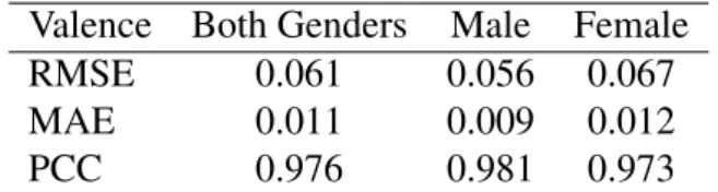
5.1 The quadrants in the Circumplex Model of Affect. . . 34 5.2 A heatmap of the true value against the predicted value for Valence for the

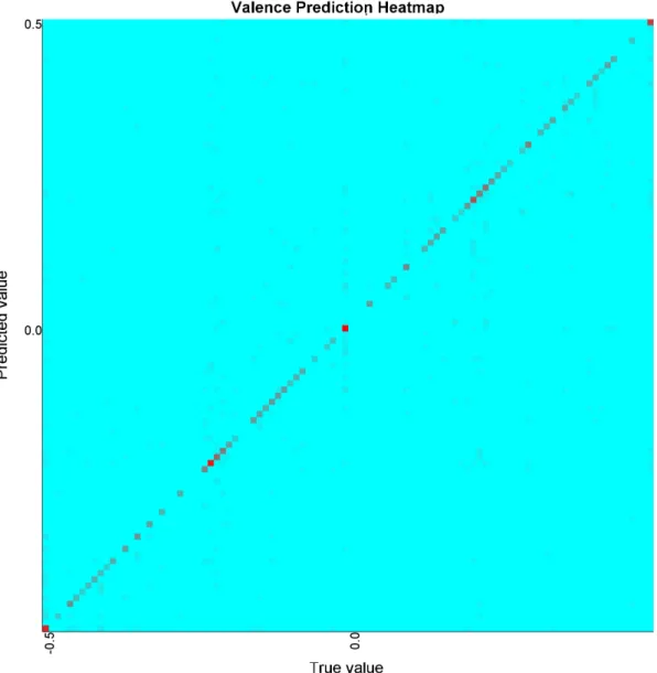
AMIGOS dataset. . . 36 5.3 A heatmap of the true value against the predicted value for Arousal for the

AMIGOS dataset. . . 37 5.4 A heatmap of the true value against the predicted value for Valence for the

DEAP dataset. . . 39 5.5 A heatmap of the true value against the predicted value for Arousal for the

DEAP dataset. . . 40

(14)

(15)

List of Tables

2.1 Table of the results obtained by Zhang, et al. Image adapted from [35]. . . 11

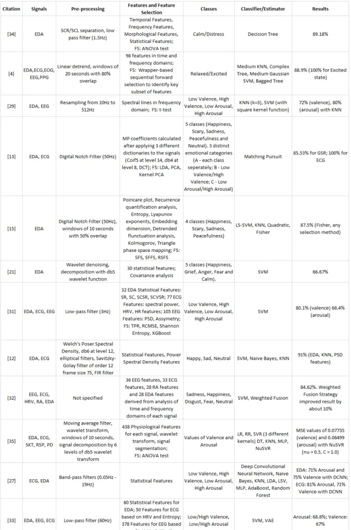
2.2 Table summarizing the methods used in works that use EDA. . . 14

3.1 Preliminary results for Valence . . . 19

3.2 Preliminary results for Arousal . . . 19

3.3 Preliminary results for the generic Valence Estimator. . . 20

3.4 Preliminary results for the generic Arousal Estimator. . . 20

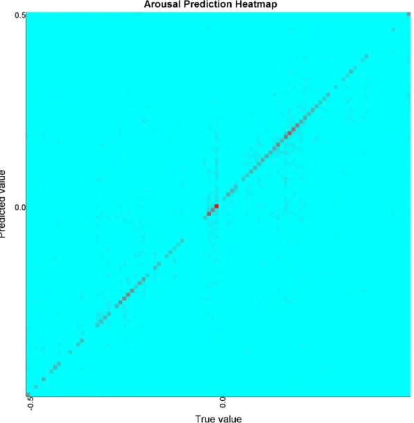
5.1 Estimation results for Valence on the AMIGOS dataset. . . 35

5.2 Estimation results for Arousal on the AMIGOS dataset. . . 35

5.3 Accuracy for High/Low classification for the AMIGOS dataset. . . 35

5.4 Classification Results for the AMIGOS dataset. . . 36

5.5 Confusion Matrix for Both Genders in the AMIGOS dataset. . . 37

5.6 Confusion Matrix for Male in the AMIGOS dataset. . . 37

5.7 Confusion Matrix for Female in the AMIGOS dataset. . . 38

5.8 Estimation results for Valence on the DEAP dataset. . . 38

5.9 Estimation results for Arousal on the DEAP dataset. . . 38

5.10 Accuracy for High/Low classification for the AMIGOS dataset. . . 38

5.11 Classification Results for the DEAP dataset. . . 39

5.12 Confusion Matrix for Both Genders in the DEAP dataset. . . 40

5.13 Confusion Matrix for Male in the DEAP dataset. . . 41

5.14 Confusion Matrix for Female in the DEAP dataset. . . 41

5.15 Comparison between our results for binary High/Low classifications and other researchers. . . 42

5.16 Comparison between estimation results. MSE values presented in Zhang, et al.’s work[35] were recalculated into RMSE. . . 42

(16)

(17)

Chapter 1 Introduction

In this introductory chapter we give a brief overview of our work. First, we present the mo-tivation that brought about this work. Afterwards we state our goals for the work, summarize the main contributions of this work and enumerate some of the results obtained. Finally, we describe how the rest of the document is structured.

1.1 Motivation

Emotion recognition has become an important research area. Being able to pinpoint accurately what emotion a person is experiencing has been shown to be beneficial in many different scenar-ios, such as improving the effectiveness of therapy sessions, gathering feedback on how users perceive certain media such as advertisements or software interfaces and even dynamically ad-justing content in a videogame depending on how a player feels. Therefore, it is useful to have computer systems that can automatically detect emotions being felt by people.

However, research done tends to have a few problems. Researchers generally identify only sets of five or less different emotions, limiting the amount of emotions that can be estimated. The second problem is that even though research has shown males have different physiological reactions than females for the same emotion, many works combine the two without analysing if their algorithm loses accuracy by doing so. The third problem is that researchers ignore the time taken by algorithms to compute the emotion based on the subject’s physiological signals, which is fundamental to obtain real-time results.

In addition, the development of emotional recognition algorithms is complex. To make it easier, many researchers plan their system structure before implementing it. However, these systems are specific to the researcher’s solution and usually not public. Therefore, it is useful to have a general purpose framework that can support the development of different algorithms. This work was conducted at LASIGE, a research unit at the the Department of Informatics, Faculty of Sciences, University of Lisbon, in the context of the project Awareness While Expe-riencing and Surfing On Movies through Emotions (AWESOME), supported by the Fundação para a Ciência e Tecnologia (FCT) under LASIGE Strategic Project - UID/CEC/00408/2019, and under project AWESOME - PTDC/CCI- INF/29234/201.

(18)

Chapter 1. Introduction 2

1.2 Goals

The main goal of this work is to develop an algorithm that can determine a subject’s emotional state after being exposed to a stimuli (e.g. image, video, sound, etc.) from their physiologi-cal signals. In particular, we use Electodermal Activity (EDA), also known as Galvatic Skin Response to estimate the emotional state for a rich set of emotions and in real-time. Addition-ally, we want to develop a software framework to make the creation and testing of emotion recognition algorithms easier and faster. To fullfill this, the following secondary goals must be accomplished:

• Research current methods for recognizing emotions from physiologicals signal and de-termine which are most useful for our goal;

• Design and implement the framework;

• Implement the algorithm for emotion estimation according to the methods identified in the research;

• Build experiments to evaluate and validate the algorithm, and determine if separating male and female subjects improves results.

1.3 Developed Solution

As mentioned in the previous section, our solution is split into two parts: a framework that supports the development of algorithms for emotional recognition, and an algorithmic process that identifies the emotional state of subjects based on their physiological signals.

The developed framework is composed of several blocks, each representing an independent part of the emotion recognition process. These blocks are Signal Feed, Preprocessor, Feature Extractor, Estimator and Results. The blocks can be connected between each other, making it simple to create emotional recognition algorithms and experiments.

The algorithm for emotional recognition was built using this framework, based on the results of the research on the current state of the art. Specifically, we start by gathering the signal from a dataset, then we split the signal into five second segments with 2.5 seconds of overlap and denoise each segment individually with the Daubechies4 wavelet. Then we extract six time-based statistical features and finally use those features to train and estimate with decision trees. In order to obtain a richer set of emotions, instead of identifying individual emotions, we estimate values for Valence and Arousal, which are described in a 2D space. Thus, with an estimated value for Valence and another for Arousal, any emotion can be represented, providing us with a richer emotional space.

(19)

Chapter 1. Introduction 3

1.4 Main Contributions

This work has two main contributions. The first is the creation of an algorithm for estimating people’s emotional state, that is a new combination of methods already used in previous works, but selected and combined to achieve good results and performance in real-time. The estimated values, on average, have very low deviation from the expected values, allowing the algorithm to obtain high accuracies. Some of the gender-specific estimators obtained slightly better results while others achieved slightly worse results, but the difference was not significant.

The second main contribution is the new framework for emotional recognition which al-lows building algorithms in a simple and fast way, as well as to perform experiments easily. The framework helps making more efficient algorithms, since it has parallelized components that quickly trade data through communication channels. With the help of this framework the algorithm executes efficiently, with the first prediction taking below 100ms and every subse-quent predictions taking less than 10ms.

1.5 Document Structure

This document is composed by six chapters.

In the first chapter, Introduction, we present the motivation and goals of the work, as well as a summary of the solution and the main contributions.

In the second chapter, Background and State of the Art, we analyze the research that has been done in the area.

In the third chapter, Algorithm for Estimation of the Emotional State, we take our find-ings from the second chapter and choose the algorithms we will use in our work

In the fourth chapter, Emotional Recognition Framework, we detail the framework we built to aid in constructing our algorithm.

In the fifth chapter, Evaluation, we present our results.

Finally, in the sixth chapter, Conclusions and Future Work, we summarize and take con-clusions about the work and its future.

(20)

(21)

Chapter 2 Background and State of the Art

As mentioned in Chapter 1, the first step to determine the algorithm for emotional recognition was to examine the current state of the art in emotional recognition from physiological signals. In this chapter we describe the current state of the art, starting by giving some background about the way emotions are represented. Then we discuss the physiological signal we chose for this work, Electrodermal Activity, and list methods to pre-process the signal, the kind of features typically used, how features are selected and which estimators are most used, and then present some works that use EDA. Afterwards we give a brief overlook of other signals that could have been chosen. Finally we summarize and discuss our findings.

2.1 Representation of Emotions

In order to estimate emotions, researchers have to describe emotions using models. There are two common approaches to achieve this.

The first approach is to choose a set of distinct emotions. Researchers estimate for limited sets of two[34][4], three[12], four[15][17] or five[13][21][32] emotions. Although there are some researchers who use more emotions, there are two problems. The first problem is that more emotions can make estimation less accurate. The second problem is that the datasets used do not have enough data for the less common emotions, and thus is not possible to train a balanced model[32].

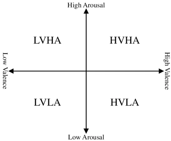
The second approach is to define emotions according to the Circumplex Model of Affect[25]. This model maps emotions in a 2D space, where the vertical axis represents Arousal and the horizontal axis represents Valence. Arousal represents how intense an emotion is and Valence says whether the emotion is negative or positive. The placing of some emotions in this model can be seen in Figure 2.1.

Researchers estimate emotions based on the Circumplex Model of Affect in two different ways. One option is to have Low and High for both Arousal and Valence as classes, for a total of four classes, and then classify which quadrant the emotion is in. This can be done with Arousal and Valence combined[13] or separately[13][30][35][31]. When classified separately, the results may be joined to obtain the corresponding quadrant[29]. The other option is to estimate values of Arousal and Valence to obtain specific positions in the 2D space[23]. This

(22)

Chapter 2. Background and State of the Art 6

approach provides a richer description of the emotional state and will be the one used in our work.

Figure 2.1: Visual representation of the Circumplex Model of Affect. Image adapted from [3].

2.2 Electrodermal Activity

Electrodermal Activity, or Galvanic Skin Response, refers to the change in sweat gland activity. Research has shown that this change reflects the intensity of the emotional state, making EDA a good measure of Arousal [26]. Because of this, EDA has become a common physiological signal to use for emotional estimation.

To estimate emotions, researchers use a series of steps which can be generalized into four groups. First, the signal, obtained either through a dataset or by an experiment, is pre-processed, which typically involves transforming the signal to remove discrepancies induced by factors other than the stimulus. Afterwards its features are extracted. Some researchers then opt in using methods to perform feature selection. Finally, the features are given to a classifier or estimator, for training or classification/estimation. The next sections present several techniques used in each of these steps.

2.2.1 Pre-processing

As mentioned before, the goal of pre-processing is to ensure the signal is prepared for the extraction of its features. A signal may, for example, have noise or interference that needs to be removed, or it may be too long and need segmentation for better feature extraction.

A common method to deal with interference is noise removal. To remove noise the common approach is to use filters. Low-pass filters attenuate the signal when frequencies above a given frequency, while high-pass filters attenuate the signal under a given frequency. Band-pass filters act as both a low-pass and high-pass filter. EDA signals do not overlap with other signals in the band 0.08-0.2Hz[21]. Researchers however use different cut-off values. Wang et. al use a

(23)

low-pass filter 3Hz cut-off[31], Zangr´oniz et al. use a low-pass filter with 1.5Hz cut-off[34], Yang et al. use a low-pass filter with 60Hz cut-off[33] and Das et al. use an elliptical filter, a kind of band-pass filter, with 10Hz cut-off[12]. Notch filters, which are a type of band-pass, are frequently used to remove inaccuracies caused by the hardware collecting the signal. Some researchers opt to use a powerline notch filter to remove powerline interference[15]. Powerline interference has a frequency of 50Hz to 60Hz[15], so researchers use cut-off frequencies like 48-52Hz[29] and 50Hz[13]. Another common way to remove noise is through the use of wavelet smoothing [21][35], which also functions as a band-pass filter[21]. The most common wavelets to smoothen EDA signals are Coiflet and Daubechies.

EDA signals are composed by two different components: skin conductance response (SCR) and skin conductance level (SCL). SCL can be seen as a ”baseline” for skin conductance, which varies between different people but very little for the same person depending on their physio-logical state, while the SCR reflects most of the change in the signal. One approach, used by Zangr´oniz, et al., was to separate these two components using a deconvolution operation so the SCR can be analyzed by itself[34]. The researchers note that this method achieves better performance at the cost of more intensive signal processing.

Depending on the dataset or the equipment, the signal may be collected at higher frequencies than needed. On higher frequencies, constant small flunctuations of the signal are considered noise, so some researchers choose to downsample their data. A technical report by researchers from the University of Birmingham, UK, suggests that because EDA signal does not change very quickly, sample rates as low as 70Hz are typical, though it is recommended a sample rate of 200Hz - 400Hz for separation of the SCR and SCL[8]. Many researchers use frequencies in the range of 128Hz - 256Hz[32][4], though some use higher[13][15] and some use frequencies as low as 10Hz[34][29].

As with other kinds of signals, a common approach for analysis of data that is longer than a few seconds is to split the data into smaller segments, also called epochs. Typically these segments have some overlap with the previous and the next segments. Segment length and overlap varies between works. For segment length, researchers generally use lengths between five and twenty seconds. For overlap, 50% overlap is common, but Anderson, et al. claimed to achieve better results with twenty second segments and 80% overlap[4]. This approach is used to provide analysis of smaller segments of the signal, from which more meaningful information can be extracted.

2.2.2 Feature Extraction

Features are extracted from the pre-processed signal and then used to train a machine learning model or to get an estimation from it. There are many kinds of features and researchers select many of them for their procedures, including:

• Time-based statistical features - these features are simple to calculate and are used by many researchers[34][21][4][21][35][27]. Examples of time-based statistical features in-clude maximum, minimum, dynamic range, mean, standard deviation, kurtosis and

(24)

skew-Chapter 2. Background and State of the Art 8

ness. Some researchers extract these features from the first and second derivatives of the signal[34][32].

• Frequency-based statistical features - Frequency-features can be extracted from the signal by first applying methods such as Fast Fourier Transform or Power Spectral Density to obtain the frequency-domain representation of the signal and then extracting features like spectral power[31]. Researchers also commonly use the same kind of features as the time-based features to extract further information from the frequency-domain signal[28].

• Entropy-based features - Entropy-based features, which analyze the irregularity of the signal, are also very used[30][4][31][15]. Many kinds of entropy features are used, like Sample Entropy, Approximate Entropy, Low Energy Entropy, Shannon Entropy, etc.

• Other features - Many works use various types of features other than the previous three, but they are not as frequently used as these. Some methods, like Poincar´e Plots, are often used to plot variations in heart rate extracted from ECG signals, but are not as commonly used for EDA signals, though some researchers use them to plot variation in EDA signals[15]. Other less common methods include Recurrence Quantification Analysis, Lyapunov exponents, Detrended Flunctuation Analysis, Kolmogorov, Trian-gle Space Mapping[15], Wavelet Transform[14], Hjorth Features and features related to Mel-frequency cepstrum[28].

2.2.3 Feature Selection

During the Feature Extraction process, researchers often extract several features. However, with the increase in the number of features comes an increase in the complexity of training the classifier or estimator. To reduce the dimensionality, a number of feature selection methods can be applied. One method is to calculate statistical significance between different classes and then analyze the results to determine the most important features[34][35]. However, for a big number of features and many possible estimation labels, this process can be very complex. One possible solution is to apply methods like Principal Component Analysis (PCA) or Linear Discriminant Analysis (LDA). PCA automatically optimizes the covariance and LDA maximizes linear class differentiation in a low-dimensional space[13].

2.2.4 Classifiers and Estimators

As mentioned in the Emotion Estimation section, most of the research estimates emotions with classifiers, which choose a result from a limited number of possibilities. For regression, re-searchers use estimators based on the same principles as the classifiers.

Support Vector Machines (SVM)[7] define an hyperplane that separates two classes in a way that minimizes incorrect predictions. Because of this its training process can take a long time, but predictions are significantly quicker.

(25)

K-Nearest Neighbors (KNN)[6] are a simple classifier that calculates the distance between every other point to calculate its nearest neighbors. In classification problems, these neighbors are used to determine the class by checking the number of occurances for each class among the neighbors. In regression problems it is similar, but instead of calculating the class it averages the values corresponding to the neighbors to determine the estimation. While simple, with a lot of data it tends to be slower than the alternatives, as it must check against every data point every time it estimates.

Decision Trees[6] are classifiers that build a set of splitting nodes. Each node checks if the value of a feature is higher or lower than a threshold and chooses the next node to check based on the result. Since every node is a simple comparison, it runs very quickly.

Random Forests[20] are classifiers that internally use a number of Decision Trees. Each tree is randomly assigned a subset of features to get an estimation, and the final estimation is the combination of the results. This method overcomes some common problems that Decision Trees have with overfitting and usually improves results[20].

Naive Bayes[22] is a probabilistic classifier where each feature contributes a certain prob-ability that one data point is from a class. It is still used, though research has shown that most recent classifiers outperform it on average[9].

Other less used classifiers include Matching Pursuit, Quadratic classifier, Fisher classifier, various methods based on neural networks such as Multi-Layer Perceptron and Deep Convolu-tional Neural Networks, and boosting-based techniques like AdaBoost and XGBoost.

2.3 Main EDA works

In the previous section we presented various methods that researchers use for each of the steps of the algorithm. In this section, we present a few works that obtained the best results for the overall algorithm for emotion recognition.

Zangr´oniz, et al. researched the possiblity of using GSR to determine if participants are feeling calm or distressed when presented with image stimuli[34]. The raw signal was pre-processed by applying a low-pass FIR filter with 1.5Hz cut-off to decrease noise. The signal was then decomposed with a deconvolution operation, separating the SCL and SCR. The features used were time-based statistical features computed over the SCR component, which were then selected by applying an ANOVA test and discarding those that were not statistically significant. Using a Decision Tree as classifier, they obtained the overall classification accuracy of 89%.

Das, et al. researched the use of GSR and ECG separately and combined to classify three emotions (happy, sad, neutral)[12] on signals obtained from visualization of 154-second long videos. Elliptical filters with frequency cut-off at 10Hz was used for the EDA signal. For the ECG signal, wavelet decomposition at level 12 was applied with mother wavelet db6. The ECG signal was further smoothened using a Savitsky-Golay filter. An FIR filter was applied to both signals to remove high frequency interference. The features used were Welch’s Power Spectral Density at the range of 0 to 20Hz and six statistical features: mean, median, mode, variance, kurtosis and skewness. Though they classified three emotions, they opted to run their

(26)

experiments in sets of two. Their results revealed that the classification with the EDA signal was better on all feature sets and classifiers than the ECG signal. When classifying between the two extreme emotions, happy and sad, the statistical features obtained 100% accuracy with the EDA signal. When classifying between Happy and Neutral statistical features were only slightly better than PSD, with the best result of 83.13% being obtained with the SVM classifier. For the Sad-Neutral classification, KNN with PSD features obtained 100%, while the best result for the statistical features was 81.61%. When the PSD and statistical features were both used in classification, the results for Happy-Sad classification fell to approximately 78% with SVM and KNN, while Happy-Neutral improved to 90.58% with Naive Bayes, though SVM fell to 62.58%, twenty percentage points lower than the statistical features alone. Sad-Neutral obtained 100% with SVM.

Goshvarpour, et al. chose to classify four classes (Happiness, Peacefulness, Sadness and Fear) on data obtained from music stimuli. First a digital notch filter was used to remove pow-erline interference. Then the signal was split into 10-second segments with 50% overlap. Then they extracted the features using Poincar´e plot indices, Recurrence Quantification Analysis, Entropy, Lyapunov exponents, Embedding dimension, Detrended Flunctuaton Analysis, Kol-mogorov and Triangle Phase space mapping. They obtained a lot of features, for which they chose to compare three different feature selection methods: Sequential floating Forward Se-lection, Sequential Forward Selection and Random Subset Feature Selection. Finally they also chose to compare between four different classifiers: Least Squares Support Vector Machine, KNN, Quadratic classifier and Fisher classifier.The best result on average was achieved with Fisher classifier and Random Subset Feature Selection, with 87.53%, though the other feature selected methods were not far behind, with 87.42% and 87.44%.

Zhang et al., differently from most other researchers, chose to estimate values of Valence and Arousal with regression[35]. They used 5 signals: EDA, Photoplethysmography, Skin Temperature, Respiration Rate and Pupil Diameter. The signals were first denoised with a moving average filter and wavelet smoothing and then segmented into 10 second segments. Finally, the signals were decomposed by 6 levels of Daubechies5 wavelet transform. During the decomposition, high-pass and low-pass filters were used separately to collect coefficients to use for the feature extraction. For every signal, 432 statistical features were collected from the original and decomposed signals as well as 6 energy-based features. To reduce the number of features, the authors employed ANOVA analysis. The best result for Arousal was 0.02323 Mean Square Error (MSE) and 0.7347 Correlation Coefficient (CC), and a 0.01485 MSE and 0.7902 CC for Valence with NuSVR. Results for other estimators can be seen in Table 2.1.

2.4 Other Physiological Signals

As seen in some of the works presented in the previous section, Electrodermal Activity is not the only signal used for emotion recognition. Many works attempt to use two or more signals either to compare the two or to use them together in order to extract the advantages of each signal. Despite the choice of only using EDA in this work, it is still useful to analyze some

(27)

Table 2.1: Table of the results obtained by Zhang, et al. Image adapted from [35].

works that use other signals.

Electrocardiogram (ECG) is a measure of the electric activity of the heart. Heart Rate (HR) and Heart Rate Variability (HRV) can be extracted from it, which gives even more information from which features can be extracted.

Wang, et. al used ECG along with EDA and Electroencephallography (EEG) [31]. Spectral power and statistical features were extracted from ECG, including analysis of the differences between consecutive R peaks in the QRS complex, which denote heart depolarization during a heart beat. By combining the features from all three signals, the authors did binary classification for High Low and obtained 80.1% accuracy for Valence and 68.4% for Arousal.

Moharreri, et al. chose to represent the differences between successive R peaks in a Poincar´e plot and extra several features from it[23]. In the end, they estimated values of Valence and Arousal using separate Decision Trees, obtaining an MSE of 0.0536 and 0.0393 for Valence and Arousal respectively. When they convert the results to classification, they obtained an accuracy of 95.71%.

Despite there are some works with good results like Moharreri, et al., the ECG signal has the disadvantage that it requires a long time to extract some of its meaningful features. The approach used by Moharreri, et al. used 5 minutes of signal in order to obtain enough data to fill the Poincar´e plot.

Another physiological signal that could be used is Pupillometry, which measures pupil di-ameter.

Babiker, et al. had success in using slight differences in pupil diameter between positive and negative stimuli to achieve a 96.50% recognition rate in valence, in an experiment where audio stimulus was used[5].

(28)

However, pupil diameter is very influenced by luminosity, and as such, in an experiment with image or video stimuli, it would be hard to predict how much the increase or reduction of pupil diameter was due to the emotion and not the visuals[5][24][16]. Henderson, et al. did an experiment on emotional imagery, where subjects were presented with short scenarios (for example, ”You jump up and block the volleyball at the net, saving the game”) and told to imagine themselves in that scenario. One of the problems the authors had was that the scripts had to be very carefully chosen to minimize differences in brightness and contrast[16].

2.5 Discussion

In the previous sections we presented the methods and some of the works on emotional recog-nition. The main works that use EDA are summarized in Table 2.2.

Many of the works use a combination of simple and complex algorithms. Statistical-based features are simple and efficient to compute, are used in most works and generally achieve good results. However, works that combine statistical features with other kinds tend to achieved better results. In other cases, authors may calculate several features and then reduce their number by using Feature Selection algorithms. The problem of using many features and using these algorithms to reduce the dimensional space is that the calculations use a lot of computation time, which is undesireable for our work. The same problem with computation time occurs when using pre-processing methods like SCR/SCL separation. Also noteworthy that many works use the full length of the signal without segmenting it in epochs. This shows that most authors are typically not concerned with having a fast algorithm, but only in achieving the best results.

Another important aspect to highlight is the low number of emotions that are identified. Most researchers classify from two to five classes. Zhang, et al., however, estimated values of Valence and Arousal, using the full spectrum of the Circumplex Model of Affect. However, they did not combine the values of Valence and Arousal to take further conclusions on the accuracy of their solution.

Due to the wide range of methods used, it is difficult to determine which parts contribute most to get good results. Many works also use several signals, further raising complexity. Works using several signals or more complex methods do not generally obtain better results.

Finally, despite some studies that show that males and females have different physiological responses to stimuli[19], few works explore this.

2.6 Summary

In this section we took a look at some of the research that has been done in the area, and in specific, we analyzed how emotions are represented using the Circumplex Model of Affect, how EDA signals are frequently pre-processed, what kind of features are extracted, how they are selected and what are the most common estimators. We also highlighted the existence of some issues with the research, namely, the lack of attention to computing time and obtaining quick

(29)

responses, the use of few emotions and the lack of works that take differences in physiological responses between genders into account.

In the following chapter we describe the methods chosen for our algorithm, in order to overcome the issues related to computation time, number of emotions and gender specificity.

(30)

(31)

Chapter 3 Algorithm for Estimation of the Emotional

State

In Chapter 2 we discussed the methods commonly used by other researchers to estimate emo-tions. In this chapter we choose which methods to use. First we discuss the methodology used for the creation of the model. Afterwards, we define a number of requirements that real-time estimation imposes. Then we present the dataset with EDA signals used to tune the model and the metrics to evaluate it. Finally, we present the methods selected to be used in our algorithm.

3.1 Methodology

As mentioned in Chapter 2, emotional estimation algorithms follow a number of steps for their creation.

The first step is collecting the data. This can be done in one of two ways. The first is by conducting an experiment where people’s physiological signals are collected while they receive some kind of stimulus, usually video, audio or image, and then are prompted to rate the emotion they felt. The second way is to use pre-existing datasets that already have this type of information. In our work, we will use pre-existing datasets.

The next steps, as described in Chapter 2 are: pre-processing, feature extraction and esti-mation. The methods were chosen by analyzing other works to find which methods are most common and have the best results. Then we choose the quickest of these, while performing tests to verify that they achieve good results. The methods chosen for each of these steps are detailed in the section Method Selection.

3.2 Real-time Estimation Requirements

As mentioned in Chapter 2, most research done has focused on developing techniques for iden-tifying emotions from a small set of emotions and without paying attention to the time required to compute it. However, to achieve real-time estimation, there are several requirements that must be fulfilled:

(32)

Chapter 3. Algorithm for Estimation of the Emotional State 16

• Fast pre-processing. For this, a windowing technique that extracts the signal in small segments (epochs) may be beneficial, as it can start pre-processing parts of the signal while it is still being captured. Other techniques that improve accuracy are potentially computationally expensive so it is required to ensure a good trade-off between speed and accuracy.

• Fast feature extraction. We can take advantage of the aforementioned windowing tech-nique to start extracting features while the signal is being captured, as well as paralelliza-tion to calculate as many features as possible in parallel. As with pre-processing, some features may take too long to be computed, which should be avoided.

• Fast estimation. Estimation models such as Decision Trees and SVM may finish quickly, but algorithms such as Matching Pursuit may take quite a bit longer. Furthermore, the system as a whole must be very efficient to minimize processing time.

3.3 Dataset

The dataset chosen for the selection of features and the creation of the model was the ’A Dataset for Affect, Personality and Mood Research on Individuals and Groups’ (AMIGOS)[2]. This dataset contains EDA, ECG and EEG signals from an experiment with 40 volunteers who watched 16 short videos. 27 of the participants were male and 13 were female. It provides rat-ings for Valence, Arousal, Dominance, Familiarity and Liking, as well as which basic emotion the person felt during a video out of seven possibilities: Neutral, Happiness, Sadness, Surprise, Fear, Anger, and Disgust. The ratings were collected through self-reporting. The values for Valence and Arousal were used in our work. In the dataset these values are in the range [1-9], but we recalculated them to fit the range [-0.5,0.5] to keep it consistent with other works.

The dataset is available in two forms: raw signals or pre-processed. In our work we used the raw version.

3.4 Metrics

To evaluate the quality of our algorithm we used the most common metrics to evaluate regres-sion estimation (RMSE, MAE, PCC). In the following equations, y represents a series of N true values for the estimation, while ˆy represents a series of N predictions from the estimator.

• Root Mean Square Error is commonly used to determine the accuracy of a regression model. Values closer to 0 mean the model has less deviation in its results;

RM SE = s

PN

i=1(ˆyi− yi)2 N

(33)

• Mean Absolute Error tells the average of the error between the estimation and the ex-pected (real) value. Values close to 0 mean that the average error is low;

M AE = PN

i=1|ˆyi− yi| N

• Pearson Correlation Coefficient is a measure of linear correlation. Values closer to 1 show that the model has strong linear correlation.

P CC = PN i=1(ˆyiyi) − PN i=1yˆi PN i=1yi q NPN i=1yˆ2i − ( PN i=1yˆi)2 q NPN i=1y2i − ( PN i=1yi)2

In addition, the estimated values will be converted into quadrants in the VA space, for which classification measures can be used to verify the accuracy of the algorithm at estimating the correct quadrant. The measures used for this are the following:

• Precision, which is the percentage of elements that were estimated for a class and truly belonged to that class;

P recision = T rueP ositive

T rueP ositive + F alseP ositive

• Recall, which is the percentage of elements that belong to a class and were estimated for the correct class;

Recall = T rueP ositive

T rueP ositive + F alseN egative

• F1 Score, which is the harmonic mean of Precision and Recall;

F1 = (

Recall−1+ P recision−1

2 )

−1

• Accuracy, which is the percentage of correctly classified elements.

Accuracy = T rueP ositive + T rueN egative

T rueP ositive + F alseP ositive + T rueN egative + F alseN egative

Finally, time between stimulus and estimation response will be measured to evaluate if the algorithm can be used in real-time estimation.

3.5 Method Selection

In this section, we will look over the methods mentioned previously and choose the most ade-quate ones to achieve these requirements.

(34)

3.5.1 Pre-processing Methods

In Chapter 2 we described the most common pre-processing methods. To make the choice for our methods, we analyzed them, taking our purposes into account.

As mentioned before, one of our goals is to make the estimations in real-time. To achieve this we are unable to use the entire length of the signal, as that would only give an estimation at the end of the stimulus. In our case, we want several estimations over time. Typically, one every few seconds, to get a better idea of how a person feels at each point of the video. Researchers typically segment the signals in 10 or 20 seconds with 50% overlap, which we consider to be too long for localized estimations. On the other hand, a researcher using the AMIGOS dataset used a window of 2 seconds[28]. In the end, we chose a compromise length of 5 seconds with 50% overlap, as it provides a balance between the amount of data available and the speed at which estimations are done.

In addition to segmenting the signal, some noise removal or baseline removal can be done. SCR/SCL separation use a computationally expensive deconvolution operation[34], so we are not using it. We decided to use wavelet denoising, which smoothens the wavelet and attenuates odd frequencies in a similar way to a band-pass filter, without being computationally demand-ing. The most used wavelet family to denoise EDA signals is Daubechies. Although researchers use db4, db5 and db6, we found that db4 was the one that most accurately describes the EDA signal.

3.5.2 Features

In Chapter 2 we presented many kinds of features, of which we noted that the statistical time-based features are among the most used. These features obtain good results and also have the advantage that they are typically simple to calculate. A study on feature selection by Shukla, etc al.[28] showed that among different kinds of features, time-based statistical features are more likely to be chosen than other popular methods, losing out only to Mel- Frequency Cepstral Coefficient (MFCC) features. However, MFCC features are not as used and are more complex than statistical features. Thus, we chose to focus on statistical features as we have more works that use them and their calculation is faster.

In the end, the following features were chosen: maximum, minimum, range, standard de-viation, skewness and kurtosis. The maximum and minimum are, respectively, the maximum and minimum values in the epoch. Range is the difference between maximum and minimum. Standard deviation, skewness and kurtosis were calculated with the following formulas, where s is global standard deviation, {x1, x2, ..., xn} are the sequence of values in the epoch, ¯x is the average of the values in the epoch and N is the total number of values in the epoch:

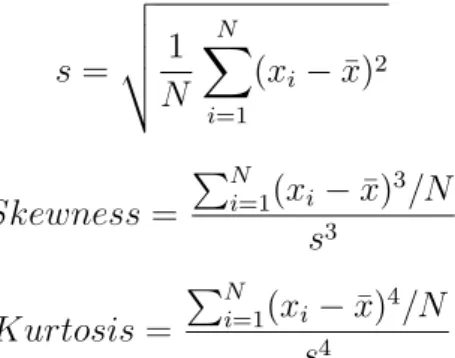
StandardDeviation = v u u t 1 N − 1 N X i=1 (xi− ¯x)2

(35)

Chapter 3. Algorithm for Estimation of the Emotional State 19 s = v u u t 1 N N X i=1 (xi− ¯x)2 Skewness = PN i=1(xi− ¯x) 3_/N s3 Kurtosis = PN i=1(xi− ¯x)4/N s4

To prevent some features having more or less importance than others, the features were normalized with the following formula, where x is the value of the feature and x0is the resulting normalized value.

x0 = ( x − mean(x) max(x) − min(x))

In preliminary tests, these features obtained the results shown in Tables 3.1 and 3.2. Other features were also tested, like area under the curve and maximum absolute deviation, but they did not improve the results.

Valence Both Genders

RMSE 0.065

MAE 0.012

PCC 0.973

Table 3.1: Preliminary results for Valence

Arousal Both Genders

RMSE 0.051

MAE 0.010

PCC 0.973

Table 3.2: Preliminary results for Arousal

3.5.3 Estimators

One of the major problems presented in Chapter 2 was that most research focused on classifying emotions from a small set of emotions. To circumvent this problem, we use regression to estimate values for Valence and Arousal. As such, we use two estimators with the same features, one for Valence and another for Arousal.

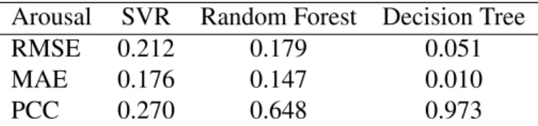
We tested some of the most popular estimators. Namely, SVR, Random Forest and Decision Tree. As we can see in Tables 3.3 and 3.4, Decision Trees obtained the best results. The SVR results are surprising, given its popularity and general success in other works. However, many kernels and parameters were tested and these were the best results found. Random Forests were tested with number of trees up to 10000. Decision Trees were also tested with up to 10000 decision nodes.

(36)

Valence SVR Random Forest Decision Tree

RMSE 0.281 0.254 0.065

MAE 0.240 0.218 0.012

PCC 0.087 0.498 0.973

Table 3.3: Preliminary results for the generic Valence Estimator. Arousal SVR Random Forest Decision Tree

RMSE 0.212 0.179 0.051

MAE 0.176 0.147 0.010

PCC 0.270 0.648 0.973

Table 3.4: Preliminary results for the generic Arousal Estimator.

3.6 Summary

In this chapter we stipulated some requirements for real-time estimation and chose the methods to use in our work, starting with the AMIGOS dataset to obtain the data, then the pre-processing of the signal, the feature extraction and the estimators. The chosen algorithm is as follows: first we segment the signal into five second windows with 50% overlap. Each window is then de-noised with a db4 wavelet. Then, the features maximum, minimum, range, standard deviation, skewness and kurtosis are extracted. Finally, the features are used to train and estimate from two Decision Trees, one for Valence and another for Arousal. The Decision Trees have a maximum of 10000 decision nodes.

While the methods chosen are not new and were used by many researchers, this combination has not been done before, due in part to our focus on real-time estimation.

We now need to build a framework with which our algorithm will be implemented, which we discuss in the next chapter.

(37)

Chapter 4 Emotional Recognition Framework

One of the problems mentioned in Chapter 2 was the lack of works relating to on real-time esti-mation. The requirements for real-time estimation mentioned in Chapter 2 presented a number of restrictions to the estimation algorithms we can use, but it also presents a challenge in how to structure the system to handle a fast estimation.

Our emotional recognition framework was conceived to tackle this challenge. The goal of this framework is to allow the user to build algorithms and experiments out of simple blocks that are all in execution simultaneously and can send data to the next blocks in the pipeline. With this system, the user can build algorithms using a sequence of blocks and use these to make experiments, and in particular, real-time experiments.

The following sections describe the arquitecture of the framework, the existing components and how to build our own emotion recognition system with it.

4.1 Framework Arquitecture

The resulting system created with the framework will be composed of several components that connect with each other to define an emotion estimation algorithm. These components are customizable, having the ability to input from or output to other components that may or may not be in use, depending on what the users need for their purposes. The connections between components are built with the following rule:

• Given component A already in the system and a component B, associate component A’s output channel X to component B’s input channel Y. Component B, if not already in the system, is added to it.

With this rule it is possible to create a variety of algorithms and experiments using these blocks. Some blocks may calculate more than one piece of information, but if the channels through which this data is sent are not connected to another component, there are mechanisms to skip their calculation, increasing performance further by only calculating what is needed.

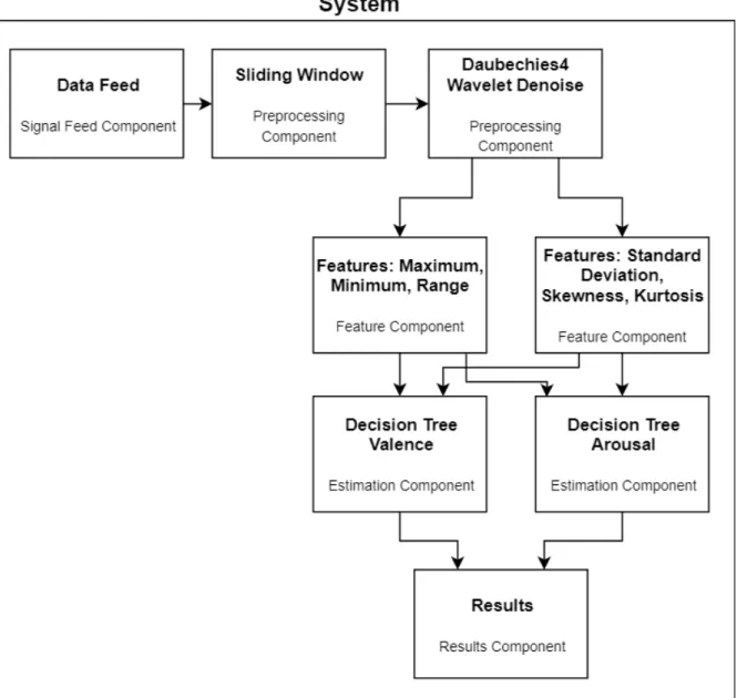
A visual representation of the algorithm and its components that we will be building with this framework can be seen in Figure 4.1.

In the next section we will describe each component in more detail.

(38)

Chapter 4. Emotional Recognition Framework 22

Figure 4.1: Diagram of the emotion recognition algorithm defined in Chapter 3 built in our framework. Estimators for gender-specific estimation omitted.

4.2 Components

From the research in Chapter 3 it was shown that emotion recognition algorithms tend to follow a similar flow - the signal is obtained, then preprocessed, then its features are extracted and finally the estimator is trained and used. The components of the framework, described in this section, follow this exact structure, making it simple for an user experienced in the area to understand where each component should be used.

• Signal Feed - This component receives signals from a data source, which can be a dataset or a device capable of extracting live physiological data, and passes it to the next com-ponents. It is also responsible for passing other information that may be necessary, for example gender, which may be necessary for experiments that have separated datasets depending on specific parameters not included in the signal itself.

(39)

• Preprocessor - This component is responsible for receiving the data sent by the Signal Feed and preparing it for the Feature Extractor. Cutting the signal into epochs and filters are examples of algorithms that fit in a Preprocessor.

• Feature Extractor - This component receives data from a Preprocessor or a Signal Feed (if the original signals are already preprocessed) and does all the necessary calculations to extract the features. The extracted features are passed to the Estimator using feature-specific channels, allowing extra information to be transmited.

• Estimator - In Training Mode, this component passes the feature vectors to its internal Dataset. When there is no more data to be processed, the Dataset is normalized and it can then be saved into a file to use later in Estimation Mode. In Estimation Mode, the component builds an estimator trained with the data in the loaded Dataset. Then, each feature vector received is normalized according to the data obtained when the Dataset was normalized in Training Mode and is then estimated using the estimator. This component is therefore responsible for maintaining its internal Dataset, training an estimator with machine learning techniques and performing the estimation to obtain the results. These are then passed to the Results component. It can also be used to perform validation, for example, using cross-validation.

• Results - This component contains the results of the estimation or validation performed by the Estimator. This is the ’output’ component which gives the user results or statistics. • System - This component controls the emotion recognition algorithm. It is responsible for forming the connections between components, starting and ending the execution of the components, and determining the Execution Mode.

4.3 Using the Framework

Using the framework is simple and requires only a few steps. The first step and most technical is the definition of the components. The second step is to use these components to define the algorithm, after which the algorithm can be executed. In the next sections we show some useful functions provided by the Component class and then show how to build the different kinds of components and how to build an emotion recognition system.

4.3.1 Component Class Functions

The Component parent class defines a few functions that are useful to control communication and execution. For communication, two simple functions are provided:

p u b l i c v o i d s e n d (d o u b l e v a l u e , i n t c h a n n e l ) t h r o w s C h a n n e l E x c e p t i o n

p u b l i c v o i d s e n d (d o u b l e[ ] v a l u e s , i n t c h a n n e l ) t h r o w s C h a n n e l E x c e p t i o n

These functions, as their name indicates, send one value or a set of values to a specific channel. These functions are the mechanism through which data is sent to other components.

(40)

Several components can be defined to read from the same channel, as will be discussed in section 4.3.7.

p u b l i c b o o l e a n i s C h a n n e l O p e n (i n t c h a n n e l )

This function checks if a particular channel is in use by the algorithm. This is useful in sev-eral cases, for example, a Signal Feed component that is designed to send sevsev-eral physiological signals through their specific channels, but an algorithm that uses that component does not use all of its signals. Thus, by using this check, the unnecessary signals and calculations can be skipped.

p u b l i c Queue g e t I n p u t Q u e u e (i n t c h a n n e l ) t h r o w s C h a n n e l E x c e p t i o n

This is a vital function that gives a component access to its internal input queues. Each channel has an input queue where values are stored until the component retrieves them.

p u b l i c v o i d c l o s e ( )

p u b l i c v o i d c l o s e I f N o I n p u t s ( )

These functions close the component, terminating their execution. The first, close(), should be run as the final function in a component to mark it as closed. It can be seen as a forced shutdown in other situations. The second one marks the component as closed only if the com-ponents that transmit data to it are already closed and there are no more values in the input queues.

p u b l i c b o o l e a n c l o s e d ( )

This function checks if the component is marked as closed and all of the components that transmit data to it are closed too. This control function is useful to determine if the component should stop executing.

4.3.2 Building Signal Feed Components

This component acts as the data entryway of the system. In order to build our own component, we must first take note of the constructor of the abstract class that defines a Signal Feed, which is as follows:

p u b l i c S i g n a l F e e d ( S t r i n g name , i n t n u m O u t C h a n n e l s )

This constructor has two parameters: a name only has significance for error checking, such as a component that has not been properly set up, and an integer value that defines the number of exit channels the component has. This number defines how many channels the component can send data through.

To build our own Signal Feed component it needs to extend the SignalFeed class and define its own constructor which defines at least these parameters. The following is an example of a constructor for a component named AMIGOSFeedAllData.

p u b l i c AMIGOSFeedAllData ( S t r i n g name , i n t [ ] w i n d o w s i z e , i n t [ ] s l i d e s i z e ) {

s u p e r( name , 7 ) ; }

(41)

This component can be created by giving it a name and two arrays. These arrays are the size of the window and how many values are discarded after each window is complete, and these values are used to determine how many segments there are in each video.

Because the programmer knows how many channels the component will have, the value can be defined here. This component has seven channels, only three of which are used in this example (1 for the EDA signal, 3 for the expected arousal and 4 for the expected valence).

The next part of the definition of a component is the definition of the run() function. @ O v e r r i d e p u b l i c v o i d r u n ( ) { / / [ . . . ] f o r (i n t i = 0 ; i < NUM USERS ; i ++) { / / o p e n u s e r d a t a f i l e d a t a s t r e a m = new B u f f e r e d R e a d e r (new F i l e R e a d e r ( d i r e c t o r y + ” g s r ” + ( i + 1 ) + ” . c s v ”) ) ; f o r (i n t j = 0 ; j < NUM VIDEOS ; j ++) { / / g e t t h e number o f s a m p l e s i n t h e v i d e o S t r i n g l i n e = d a t a s t r e a m . r e a d L i n e ( ) ; S t r i n g [ ] s p l i t = l i n e . s p l i t (” ”) ; d o u b l e r o w s = D o u b l e . p a r s e D o u b l e ( s p l i t [ s p l i t . l e n g t h − 1 ] ) ; / / g e t number o f windows i n t h e v i d e o s i z e = (i n t ) r o w s / s l i d e s i z e [ s ] −( w i n d o w s i z e [ s ] / s l i d e s i z e [ s ] ) −1; f o r (i n t z = 0 ; z < r o w s ; z ++) { / / s e n d v a l u e t o n e x t c o m p o n e n t l i n e = d a t a s t r e a m . r e a d L i n e ( ) ; s p l i t = l i n e . s p l i t (” ”) ; / / s e n d EDA s e n d ( D o u b l e . p a r s e D o u b l e ( s p l i t [ 2 ] ) , 1 ) ; } f o r(i n t m = 0 ; m < s i z e ; m++) { / / s e n d s e l f a s s e s s m e n t v a l u e s o f a r o u s a l and v a l e n c e , n o r m a l i z e d f r o m [ 1 , 9 ] t o [ − 0 . 5 , 0 . 5 ] s e n d ( ( ( s e l f a s s e s s m e n t [ i ∗NUM VIDEOS+ j ] [ 3 ] − 1 ) / 8 ) − 0 . 5 , 3 ) ; s e n d ( ( ( s e l f a s s e s s m e n t [ i ∗NUM VIDEOS+ j ] [ 4 ] − 1 ) / 8 ) − 0 . 5 , 4 ) ; } } / / [ . . . ] c l o s e ( ) ; }

The programmer can then define the code as they wish: either by extracting the data from a dataset or collecting it with hardware in real-time, using the APIs provided for the purpose. In this excerpt, the dataset was processed beforehand to facilitate its processing in the code.

(42)

At the end of the run() function the close() function should be run to mark it as closed.

4.3.3 Building Preprocessing Components

Building Preprocessing components is very similar to building Signal Feed components. The constructor of the abstract class is the following:

p u b l i c P r o c e s s i n g C o m p o n e n t ( S t r i n g name , i n t n u m I n C h a n n e l s , i n t

numOutChannels , i n t n u m S a m p l e s B a s e l i n e , i n t n u m S a m p l e s S t i m u l u s )

This constructor has three more values. The first is numInChannels. Like numOutChannels is for the number of exit channels to send values to other components, numInChannels is the number of entry channels through which a component can receive values. The next two values are used to specify the number of samples that the signal has for baseline calculations and the number of samples of stimulus. Depending on the algorithm, these two may not be used.

The following is an example of a constructor for a component named Daubechies:

p u b l i c D a u b e c h i e s ( S t r i n g name , i n t n u m S a m p l e s B a s e l i n e , i n t n u m S a m p l e s S t i m u l u s , i n t w a v e l e t ) { s u p e r( name , 1 , 1 , n u m S a m p l e s B a s e l i n e , n u m S a m p l e s S t i m u l u s ) ; t h i s . w a v e l e t = w a v e l e t ; }

Like with Signal Feed components, the number of entry and exit channels is known to the programmer. In this case an extra parameter is added, making the system engineer able to create any of the different kinds of Daubechies wavelets without having to build a different component. Also like Signal Feed, only the run() function is left to define. However, in addition to using close()at the end of the function, the run() function should have a loop like the following, which allows the component to execute until it is either forcibly closed or there is nothing left for it to do. @ O v e r r i d e p u b l i c v o i d r u n ( ) { w h i l e( ! c l o s e d ( ) ) { / / c o d e h e r e c l o s e I f N o I n p u t s ( ) ; } c l o s e ( ) ; }

4.3.4 Building Feature Components

Building Feature components is similar to Preprocessing components. The constructor of the abstract class has one difference:

p u b l i c F e a t u r e C o m p o n e n t ( S t r i n g name , i n t n u m I n C h a n n e l s , i n t n f e a t u r e s , i n t

(43)

In the Features component, numOutChannels changes to nfeatures. The name change does not affect how the component is used and merely reflects what the component itself is used. As such, building the Features component is identical to the Preprocessing component, with the exception that the Feature component can connect to the Estimation component’s feature channels.

Like numInChannels and numOutChannels in the previous two components, nfeatures is known to the programmer, so it can be defined by default, as presented in the next example of a component called MaxMinRanFeature, which calculates the maximum, minimum and range features. p u b l i c MaxMinRanFeature ( S t r i n g name , i n t n u m S a m p l e s B a s e l i n e , i n t n u m S a m p l e s S t i m u l u s ) { s u p e r( name , 1 , 4 , n u m S a m p l e s B a s e l i n e , n u m S a m p l e s S t i m u l u s ) ; }

These components should have a structure for the run() function equal to the Preprocessing components.

4.3.5 Building Estimation Components

Building the Estimation components has a few more steps. The constructor of the abstract class is similar to the previous components:

p u b l i c E s t i m a t i o n C o m p o n e n t ( S t r i n g name , i n t n u m I n C h a n n e l s , i n t

numOutChannels , S t r i n g f i l e n a m e )

Likewise, the construction of an Estimation component called RegressionTreeEstimator can be done in this way:

p u b l i c R e g r e s s i o n T r e e E s t i m a t o r ( S t r i n g name , i n t n u m I n C h a n n e l s , i n t

numOutChannels , S t r i n g f i l e n a m e )

{

s u p e r( name , n u m I n C h a n n e l s , numOutChannels , f i l e n a m e ) ; }

The Estimation Component requires the definition of more functions other than run(), namely, train(), estimate() and validate().

Another useful, already defined function is fillDataset(), which is used to fill the estimator’s internal dataset prior to the training procedure. While the training could be done at the same time, it would offer no advantage as the training process is done separetely from the estimation process, thus execution in real-time is not needed. In this way we can build the entire dataset which we can dump to a file (dump()) and restore it later to use it restore(). The file used for the dump()and restore() functions is the file specified in the filename parameter.

An example of run() function is as follows: @ O v e r r i d e

p u b l i c v o i d r u n ( ) {

EmoStatus - Estimating the emotional state of people using electrodermal activity

2019