Numerical Analysis of Wooden Slabs with Perforations Under Fire Conditions Djaafer Haddad

Numerical Analysis of Wooden Slabs with Perforations

Under Fire Conditions

Djaafer Haddad

Final Thesis Report Presented to:

Escola Superior de Tecnologia e Gestão

Instituto Politécnico de Bragança

Thesis submitted to fulfil the requirements of Ms.C degree in:

Construction Engineering

Supervised by:

Professor Elza Maria Morais Fonseca

Professor Belkacem Lamri

iii

Acknowledgements

At the end of this work, I would like to express my deep gratitude and my sincere thanks for “My Family” to their tender encouragement and their great sacrifices, they have been able to create the climate affectionate and conducive to the continuation of my studies.

My profound thanks go to my coordinators Pof. Elza Fonseca, and Prof. Belkacem Lamri, for their helps and advices given in my work and their interested to solve problems and find solutions to move forward.

Also I would like to thank all my friends, for supports and encouragement, specially Nabil.

iv Numerical Analysis of Wooden Slabs with Perforations under Fire Conditions

By: Djaafer Haddad

Thesis submitted to fulfil the requirements of Ms.C degree in: Construction Engineering

Supervised by:

Prof. Elza Maria Morais Fonseca Prof. Belkacem Lamri

Abstract:

Wood is considered an ideal solution for floors and roofs building construction, due the mechanical and thermal properties, associated with acoustic conditions. These constructions have good sound absorption, heat insulation and relevant architectonic characteristics. They are used in many civil applications: concert and conference halls, auditoriums, ceilings,

walls… However, the high vulnerability of wooden elements submitted to fire conditions requires the evaluation of its structural behaviour with accuracy.

The main objective of this work is to present a numerical model to assess the fire resistance of wooden cellular slabs with different perforations. Also the thermal behaviour of the wooden slabs will be compared considering different material insulation, with different sizes, inside the cavities.

A transient thermal analysis with nonlinear material behaviour will be solved using ANSYS© program. This study allows to verify the fire resistance, the temperature evolution and the char-layer, throughout a wooden cellular slab with perforations and considering the insulation effect inside the cavities.

v Análise numérica de lajes em madeira com perfurações em situação de incêndio

Djaafer Haddad

Dissertação para obtenção do grau de Mestre em: Engenharia da Construção

Realização sobre a supervisão de: Prof. Doutora Elza Maria Morais Fonseca

Prof. Doutor Belkacem Lamri

Resumo

A madeira é um material considerado como uma solução ideal para pisos e tetos em construção de edifícios, devido às suas propriedades mecânicas e térmicas, associada a boas condições acústicas. Este tipo de construções permite uma boa absorção sonora, isolamento térmico, com características arquitetónicas relevantes. As aplicações em construção são variadas: salas de conferência ou concerto, auditórios, tetos, paredes… Todavia, a alta vulnerabilidade dos elementos de madeira submetidos a condições de incêndio, requer a avaliação de seu comportamento estrutural com precisão.

O principal objetivo deste trabalho é apresentar um modelo numérico para avaliar a resistência ao fogo das lajes celulares de madeira com diferentes perfurações. Também o comportamento térmico de lajes de madeira serão comparadas considerando diferentes materiais de isolamento, com placas de espessura diferente no interior das cavidades.

Será utilizado o programa ANSYS© para a análise térmica e transiente com comportamento do material não-linear. Este estudo permite verificar a resistência ao fogo, a evolução da temperatura e a determinação da velocidade de carbonização, para as lajes celulares de madeira com perfurações, considerando ainda o efeito de isolamento no interior das cavidades.

vi

Index

1 Introduction ... 2

1.1 Objectives ... 5

1.2 Summary of the chapters ... 6

2 Fire Action ... 9

2.1 Heat Transfer ... 9

2.2 Modes of Heat Transfer ... 9

2.2.1 Conduction ... 10

2.2.2 Convection ... 12

2.2.3 Radiation ... 13

2.3 Fire curves ... 14

2.3.1 Standard time-temperature curve ... 15

2.3.2 External fire curve ... 16

2.3.3 Hydrocarbon curve ... 16

2.3.4 ASTM fire curve ... 16

3 Thermal Behaviour ... 19

3.1 Pyrolysis ... 19

3.1.1 Ignition ... 20

3.1.2 Char layer of wood ... 20

3.1.3 Effective char layer ... 22

3.2 Thermal properties of wood ... 23

3.2.1 Thermal conductivity ... 23

3.2.2 Specific heat ... 24

3.2.3 Wood density ... 25

3.3 Thermal properties of insulation materials ... 26

3.4 Thermal properties of air ... 29

4 Finite Element Method ... 31

4.1 Introduction ... 31

vii

4.3 Finite elements ... 35

4.3.1 Shape functions for 8 nodes (Lagrange) ... 36

4.3.2 Shape functions for 20 nodes (Serendipity) ... 37

5 Cellular Slab With Perforations ... 40

5.1 Introduction ... 40

5.2 Dimensions of the perforated wooden slab ... 40

5.3 2D cellular slab with perforations ... 41

5.3.1 Presentation of models and geometry ... 41

5.3.2 Mesh and boundary conditions ... 45

5.3.3 Results of 2D models ... 47

5.4 3D Cellular slabs with perforations ... 59

5.4.1 Presentation of models and geometry ... 59

5.4.2 Mesh and boundary conditions ... 61

5.4.3 Results of 3D models ... 62

6 Conclusions and Future Work ... 70

viii

Index of Figures

Figure 1- Conduction, convection and radiation, [20]. ... 10

Figure 2- Conductive heat transfer, [21]. ... 10

Figure 3- Forced convection, [23]. ... 12

Figure 4- Natural convection, [24]. ... 12

Figure 5- Fire development, [22]. ... 14

Figure 6- Standard time-temperature curve ISO 834, [6]. ... 15

Figure 7- Standard fire curves. ... 17

Figure 8- Physical degradation zones in a wooden section, [31]. ... 19

Figure 9- One-dimensional char layer of a cross section (fire exposure on one side), [15]. ... 21

Figure 10- Char layer depth when fire exposure more than one side, [15]. ... 21

Figure 11- Definition of residual cross-section and effective cross-section, [15]. ... 22

Figure 12- Variation of k0: a) for unprotected members and protected members where tch >20 minutes, b) for protected members where tch > 20 minutes. ... 23

Figure 13- Thermal conductivity as a function of temperature. ... 24

Figure 14- Specific heat as a function of temperature. ... 25

Figure 15- Density coefficient as a function of temperature. ... 26

Figure 16- Medium fibre density and mineral wool [34]. ... 28

Figure 17- Boundary conditions for thermal problems in the field Ω, [41]. ... 32

Figure 18- PLANE77 geometry, [43]. ... 35

Figure 19- SOLID90 3-D 20-Node Thermal Solid [43]. ... 36

Figure 20- Constructive models of wooden slabs, [27]. ... 40

Figure 21- Wooden slab with cellular zones, [14]. ... 41

Figure 22- a) Wooden cellular slab: rectangular perforation. ... 42

Figure 23- Mesh of finite element, plane77. ... 45

Figure 24- Temperature curves used inside the cavities in numerical analysis. ... 46

Figure 25- Curves of fire exposure ‘’Furnace’’ and ISO 834. ... 46

Figure 26- Temperature and residual cross-section of slab using MDF, at 400s. ... 50

Figure 27- Temperature evolution and residual cross-section of slab using MDF, at 1800s. .. 51

Figure 28- Comparison of temperature distribution between RW and MDF, time 1800s. ... 52

Figure 29- Residual cross-section of wooden slab with perforations with RW and MDF. ... 52

ix

Figure 31- Time-temperature in wooden slabs with and without MDF. ... 55

Figure 32- Time-temperature in wooden slabs in models with and without air. ... 56

Figure 33- Time-temperature in wooden slabs in models with RW and MDF with air. ... 57

Figure 34- Time-temperature in wooden slabs. ... 58

Figure 35- 3D model in Autocad. ... 60

Figure 36- 3D model in Ansys program. ... 60

Figure 37- Mesh, solid elements with 20 nodes, with and without insulation. ... 61

Figure 38- Temperature evolution and residual cross-section of 3D wooden slab. ... 63

Figure 39- Time-temperature history in wooden cellular slab for models 2D and 3D. ... 64

Figure 40- Temperature and residual cross-section of 3D wooden slab, MDF=36mm. ... 65

Figure 41- Time-temperature in 2D and 3D wooden slab with MDF. ... 66

Figure 42- Temperature and residual cross-section of 3D wooden slab, RW =36mm. ... 67

X

Index of Tables

Table 1: Design charring rates β0 and βn of timber, [15]. ... 22

Table 2: Determination of k0 for unprotected surfaces with t in minutes, [15]. ... 23

Table 3: Temperature-thermal conductivity relationship for wood, [15]. ... 24

Table 4: Specific heat of wood, Eurocode 5, [15]. ... 25

Table 5: Specific mass of wood, Eurocode 5, [15]. ... 26

Table 6: Overview of the insulation material properties. ... 28

Table 7: Thermal properties of air, [39]. ... 29

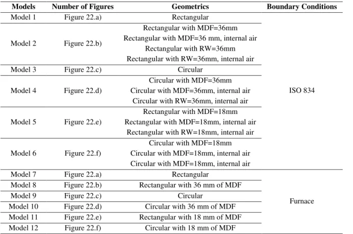
Table 8: Numerical models characterizations. ... 44

Table 9: Char layer depth. ... 47

Table 10: Charring rates values. ... 48

1

Chapter 1

2

1

Introduction

The problem of the fire resistance in wooden elements is analysed from the behaviour that the material presents when is exposed to fire action. Fire resistance relates to the period for which an element will resist to a flame passage, remains free from collapse and insulate against an excessive temperature rise of the unexposed face. Different fundamental phenomena need to be evaluated: combustion, heat transfer and wood properties degradation with temperature dependence, [1].

In this work different wooden cellular slabs are considered for study with typical applications in construction engineering, as auditoriums, offices, restaurants, concert halls, schools, hotels, gymnasiums, etc. Also they are typical panels applied in building structures with a rustic and decorative look. The combination between the wood materials and other acoustic material layers offers aesthetics and sound absorption effect. The perforations in these slabs are common and available in different patterns and sizes. Fire experimental tests in different wooden surfaces were performed by Frangi et al. [2], presenting some results of the fire tests and show a simplified calculation model for the burning rate compared with the test results. Two different charring phases were taken into account for this model. The results showed that fire penetration into the cavities of the hollows elements can be prevented, if the perforated acoustic layer and the sound absorbers placed behind it are sufficiently thick. Before and after the perforated acoustic layer is completely charred, and the fire tests clearly showed that the charring rate during the first phase is mainly influenced by the size and the position of the perforations, as well as, the thickness of the perforated acoustic layer.

3 The charring rate is strongly affected by the material density and it has been studied by different researchers. In 2008 Frangi et al [4], present research of a charring model based on an extensive finite element thermal analysis, for timber frame floor assemblies with void cavities. The results showed that the charring model takes into account the influence of high temperature after failure of the fire protective claddings, as well as, the heat flux superposition on the charring rate of the timber beams exposed to fire on three sides.

In 2003 Frangi and Fontana M. [5] were also worked on the fire behaviour of timber slabs, made of hollow core elements and of timber-concrete composite slabs contributed to the experimental database of charring and temperature measurements of wood members exposed to fire. The results showed simplified methods based on a constant charring rate to calculate the fire resistance of wood elements. They are confirmed by the fire tests with different timber members exposed to the standard ISO fire [6] of 30-110[min], also the use of a simplified method for the fire resistance of load bearing wood sections should therefore only be used up to a residual cross-section of 40-60[min]. The temperature profiles through wood members exposed to fire depend on the duration of fire exposure.

Also in 2010 Cachim P.B and Franssen J.M,[7] worked with two calculations methods from EC5. They used simplified and advanced methods for the calculation of fire resistance in timber structures. The methods are regarding the calculation of the char depth and residual cross section strength. They produced also finite element simulations, performed using the code SAFIR, the numerical results indicate that both models have some limitations. According their results some proposals to overcome the inconsistencies, as well as, to extend their applicability, namely an expression to calculate the charring rate, as a function of density and moisture content.

4 In perforated cellular wooden slabs, the size of perforations facilitates and increases the heat flow and flames penetration over the slab. An insulation material in combination with other building materials allow to reduce the heat transfer inside and outside of the element. There are many kinds of insulating materials, each of which has its own set of advantages and disadvantages, and none of which is the perfect solution. The best insulation materials should have the lowest thermal conductivity, in order to reduce the total coefficient of heat transmission. The insulation material should be rated as non-flammable and non-explosive. In the event that the insulation material burns, the products of combustion should not introduce toxic hazards. The main question is to choose the correct thermal insulation material which helps to satisfy building requirements as a mostly energy and cost efficient.

In 2013 Fonseca E.M.M., et al [10]proposed a numerical model to assess the fire safety of wooden slabs with rectangular perforations on a ceiling. An internal fibreboard insulation material was added inside cavities. Finite element program was used for nonlinear material in transient thermal analysis to allow verifying the temperature evolution, the char-layer throughout the slab and verifying the influence of the use of a fibre board. The results showed that the type and the size of perforations can limit the use of these constructive elements in terms of fire resistance. Also, the use of insulation material limits the heat penetration and the charring rate is lower. As a conclusion, the constructive elements should be chosen before, to prevent and delay the fire damage effect.

In the same year 2013 Fonseca E.M.M et al. [11] developed a numerical model to assess the fire behaviour of cellular wood slabs with different drillings. A transient thermal analysis with nonlinear material behaviour was solved with ANSYS© program. The main goal was to present a numerical model based on a constructive solution proposed by Frangi and Fontana 2004, [12] to calibrate the numerical results. The results for charring depth indicate that the numerical method reveals good performance when compared with the experimental model. In case of fire exposure, the type and size of perforations should be chosen before, allowing that the slab could remain in service during more time.

5 Additional work produced in 2015 David C., et al., namely with Meireles [14] presenting a 3D constructive models for experimental tests in laboratory, representing cellular wooden slabs but now with different circular perforations. These slabs were tested in the same fire resistance furnace, as the previous, to predict the evolution of the temperature and the charring layer in constructive solutions.

In the present work, the main goal is the use of an advanced calculation method for determining the charring depth, the profiles and the temperature distribution through the construction elements during a fire scenario. A finite element program (ANSYS©) will be used for transient and nonlinear material thermal analysis. This work describes the basic idea of a 2D and 3D numerical model, to predict the time temperature history and the residual cross-section identification in wooden cellular slabs with and without perforations. The initial validation of the numerical model will be obtained using the experimental tests from David and Meireles [13], [14]. In addition, different constructive solutions will be numerically analysed, and insulation material will be added inside the cellular cavities to determine the influence on time-temperature history. Also the cavities with insulation will be fulfil with internal air. The numerical models combine different materials, as temperature dependent and constant values. The main results of the numerical analysis are presented and the proposed 2D models are compared with 3D models to represent more realistic situation. The results enlarge the knowledge of the fire behaviour of different insulation materials applied in wooden slabs, and complete others investigations developed by the supervisors of this work.

1.1

Objectives

6 addition, all two dimensional models will be reproduced, but with different insulation material to verify the influence in fire resistance. At the last step, 3D (three dimensional) numerical models will be produced to study wooden slabs with perforations. In all numerical simulations, appropriate material properties and boundary conditions will be used to predict the real fire effect.

The main goal of this work is to present different constructive numerical solutions of wooden slabs with rectangular or circular perforations, with or without insulation material, to study the fire resistance in such way that contributes for a safe design. The subject of this work is an ongoing project, according to others investigations produced and tested in the laboratory of the Polytechnic Institute of Bragança with typical wooden slabs submitted to experimental tests, [10-11], [13-14].

During all steps of this work different programs for calculation, drawing and analysis were used. The software used in this work are the following: Excel, Autocad and ANSYS©.

1.2

Summary of the chapters

More six additional chapters will be presented in this report with all described work and steps to concretize the final master thesis.

In Chapter 2 of this work, a description of the heat transfer mechanisms by conduction, convection and radiation, will be presented. Also, parametric curves defined by Eurocode 1 part 1.2 [16], ASTM E119, [17] and the standard curve of natural fire, which characterizes the time temperature evolution, are presented.

Chapter 3 explains the thermal behaviour of materials and presents the thermal properties of wood and insulations material used in this study (MDF, Medium Density Fibreboard and RW, Mineral Wool), namely the thermal conductivity, specific heat and the specific mass.

In Chapter 4 a description of the finite element method (FEM) used in this work with

7 problems, describes the thermal diffusivity equation and presents the shape functions of the finite element for 2D and 3D meshes.

In Chapter 5 description of different 2D and 3D models is exposed based in the dimensions of a constructive real solution, for results comparison. A transient thermal analysis with nonlinear material behaviour will be developed using ANSYS© program. The char layer formation through time in wood slabs submitted to fire will be calculated. All boundary conditions are well defined and the type of results (profile of temperatures, char layer and charring rate) are presented in all slabs in study.

The last two chapters, chapter 5 and chapter 6, are related with the ‘’Conclusions and

8

Chapter 2

9

2

Fire Action

2.1

Heat Transfer

The basic development of the heat transfer is needed to calculate the char layer evolution in wood materials when submitted to fire. In general, the heat transfer is based on the principle of conservation of energy. This principle shows that the amount of energy used must be equal to the sum of the energy leaving and stored in the system. Applying the conservation principle of energy to heat transfer rates, the first law of thermodynamics could be presented as follows, [18].

dW dQ

dU   (1)

Where dU is the modification of internal energy in the system, dQ is the amount of heat added to the system; dW is the amount of work done by the first law of thermodynamics.

This law means that if no work is done by the system, the change in internal energy must equal the heat change in the system, [18]. The three components were generally implied in the heat transfer are: conduction, convection and radiation. According the definition, conduction is the mechanism for heat transfer through solid materials, convection is the heat transfer by the movement of fluids, either gases or liquids and radiation is the transfer of energy by electromagnetic waves, [18].

2.2

Modes of Heat Transfer

The heat transfer knowledge in engineering consists of the evaluation of three modes with specific conditions, properties and geometries, and with further application than that usually used to design and performance analysis of heat exchangers, [19].

10 Figure 1- Conduction, convection and radiation, [20].

2.2.1 Conduction

As defined, “Conduction is the transfer of energy from more energetic particles to less energetic ones due to interaction between atomic and molecular particles”, [19]. The conductive heat transfer is schematized in figure 2.

Conduction can occur in: solid, liquid and gaz. “In solidsconduction the heat transfer is due to the combination of vibrations of the molecules in a lattice and energy transport by free electrons”, [19]. Conduction is the diffusion and collision of molecules in gases and liquids during their random motion, [19].

Figure 2- Conductive heat transfer, [21].

11

dx dT KA

Q (2)

dx dT K

q (3)

Considering the finite slab of material shown in Figure 2, for one-dimensional conduction the temperature gradient is given by the following equation, [21].

L T T dx

dT _{ 2}  ₁

(4)

Substituting in equations 2 and 3 the transfer law can also be written:

L T T kA

Q 1 2 (5)

L T T k

q 1  2 (6)

Where A is the area through which the heats flow, in normal to the x-direction, Q is the heat flow conduction in the x-direction, q the heat flux normal to the x-direction, K is the

positive constant of the material thermal conductivity [W/m°C], dT/dx is the temperature

gradient in x-direction [K/m], T represents the temperature [°C] and L represents the thickness [mm].

12

2.2.2 Convection

Convection heat transfer is a mode which consists of two mechanisms: random molecular motion which is termed diffusion or the bulk motion of a fluid carries energy from place to place. Convection takes place between a fluid in motion and a boundary surface when they meet at different temperature, [21]. Heat transfer by convection can be classified in accordance with their nature by free convection and forced convection. In forced convection, the fluid motion is driven by some external influence (artificial), [19, 21].

Figure 3- Forced convection, [23].

In natural or ‘free’ convection, flow is induced by buoyancy forces, which are caused by variations of temperature formed due to heat transfer in the fluid, [19].

Figure 4- Natural convection, [24].

13





c T T

h

Q   (7)

Where Ts is the temperature of the surface receiving or giving heat, Tf is the average temperature of the stream of fluid adjacent to the surface, hcis the convective heat transfer coefficient which has units equal to [W/m2K]. If the fluid temperature is higher, the heat flux is given by the expression, [25].





c T T

h

Q   (8)

2.2.3 Radiation

Radiation is the energy transmits by all matter that has a nonzero temperature. This energy is transmitted in the form of electromagnetic waves. The propagation of electromagnetic waves changes the electronic configuration of atoms and molecules. Energy transfer due radiation is very efficient also in vacuum. It is considered as transfer phenomenon between solid surfaces, [19]. Stefan-Boltzmann law allows the calculation of the maximum rate of radiation of a blackbody or ideal radiator. The upper limit of emissive heat transfer is given by Stefan-Boltzmann law as, [19]

4 s

b T

E  (9)

Where Eb is the emissive power of blackbody [W/m2]; σ is the Stefan-Boltzmann constant equal to 5.6697×10-8 [W/m2K4]; Ts is the absolute temperature of the surface in [K]. “Heat flux emitted by real surface is less than that of blackbody at the same temperature and is given as”, [19].

4 s

T

14 Where E is the Emissive power of real surface [W/m2],  is the emissivity that depends strongly on material and finish of surface, which varies between zero and one.

2.3

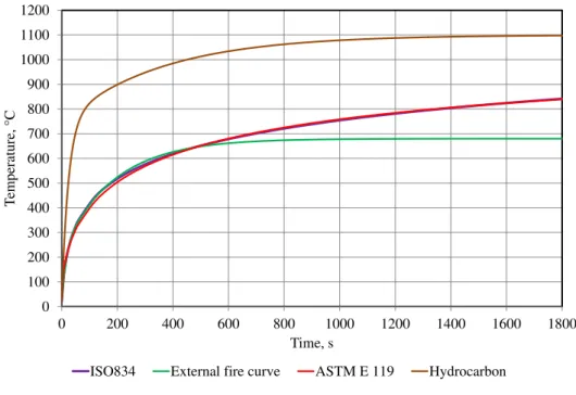
Fire curves

A natural fire occurs when there is a presence of three important causes: source of heat, fuel and oxygen. The combustion happens when these three elements are mixed at a specific temperature; the natural fire curve is divided into four successive phases: ignition, initial phase, full combustion and cooling phase, [26].

Figure 5- Fire development, [22].

15 due to a decrease in the temperature, or the fuel shortage or lack of oxygen, which may lead to extinguishing the fire, [26-27].

2.3.1 Standard time-temperature curve

The evolution of the fire temperature is defined according to the rated temperature curves as a function of time, or another shape as parametric curves defined for this purpose, according Eurocode 1 part 1.2, [16]. The fire curve ISO834 allows the development of the room temperature [28]. This curve is described by the equation 11 and represented in figure 6:





345 ₁₀

0  

T t

T (11)

Where T is the gas temperature in the compartment [°C], t is the time in [min] and T0 is the initial temperature compartment, which usually is considered equal to 20[°C].

Figure 6- Standard time-temperature curve ISO 834, [6]. 0

100 200 300 400 500 600 700 800 900

0 200 400 600 800 1000 1200 1400 1600 1800

T

empera

ture

, [

C

]

16

2.3.2 External fire curve

The external fire curve shown in Eurocode 1 part 1.2 [16], applies only for external structural elements, and the temperature is described by the equation:





8 . 3 32

.

0 _0.313

687 . 0 1

660 e e T

T     t   t  (12)

In this equation after 30 [min], temperature keeps constant at 680 [ºC]. The others parameters are T representing the gas temperature near the member in [°C] and t is the time in [min].

2.3.3 Hydrocarbon curve

The hydrocarbon curve is defined by equation 13, that is a curve which is characterized as the most energetic of all, after 30[min] the temperature remains constant to 1100[° C] according to Eurocode 1 part 1.1, [16] the equation is given by:





5 . 2 167

.

0 _0.675

325 . 0 1

1080 e e T

T     t   t  (13)

Where: T is the gas temperature in the fire compartment in [°C], t is the time [min].

2.3.4 ASTM fire curve

17





79553 .

3 _170.41

1

750 e t T

T     t    (14)

Where t represents the time elapsed since the start of the test in [min] and T0 the initial temperature of the enclosure in the [°C].

In figure 7, different curves are represented, according to the evolution of temperature versus time history.

Figure 7- Standard fire curves.

For the fire resistance of structural elements, usually the standard fire curve ISO 834, [6] is used. Although with little physics reality, it allows standardizing experimental tests, enabling the comparison of the results of fire resistance obtained in different laboratories, [29].

0 100 200 300 400 500 600 700 800 900 1000 1100 1200

0 200 400 600 800 1000 1200 1400 1600 1800

T

empera

ture

,

C

Time, s

18

Chapter 3

19

3

Thermal Behaviour

Fire is one of the great opponents of the building materials, which can be the first responsible for losing stiffness and strength for some materials like steel, also for wood when

it’s exposure to high temperatures the section gradually reduces, [27]. The timber is characterized by his low thermal conductivity. This property is used to delay the increase in temperature in the vicinity of areas that is in the combustion and prevent excessive expansion of the structure. When wood is exposed to fire, three different layers can be distinguished over the section, figure 8. The first layer is the surface characterized by carbonization. This layer function plays a role as a good thermal insulation due to its low thermal conductivity, preventing the penetration of heat into the section. The pyrolysis zone is a layer located between the charred layer and the wood core, usually with smaller thickness, where the properties are changed, but not completely decomposed. The last zone is defined inside the section where the wood does not suffer any change in its properties. This zone is the intact wooden zone, [27], [30].

Figure 8- Physical degradation zones in a wooden section, [31].

3.1

Pyrolysis

20 moisture occurs. As the temperature is raised to 200[°C] the surface layer of the wood starts to dehydrate in the absence of oxygen, this process of thermal degradation level is called pyrolysis, between 200[°C] and 280[°C], and the degradation of the surface layer moves to the inside of the timber. This region is followed by a layer in which the pyrolysis takes place slowly. Between 240[°C] and 350[ºC] there is a slow formation of char layer. In the range between 280[°C] to 500[°C], exothermic reactions produce with the release of combustible gases, in the form of smoke. Above 500[°C] it remains in the temperature elevation, to complete char layer, [28].

3.1.1 Ignition

The wood ignition happens when it is subjected to an enough high temperature with oxygen-rich atmospheres. Ignition may be two distinct types: spontaneous or provoked. Spontaneous happen in the absence of any ignition source, and the surface of the wood is ignited by any means of energy, a heat of a fire or a burning object. This flux of energy or heat may have two components, radiation and convection. The provoked ignition happens when the wood surface reaches into contact with any source of ignition, flame or spark, [28].

3.1.2 Char layer of wood

When subjected to high temperatures, wood suffers a breakdown and the formation of a layer of carbon happens. This layer plays the role of insulation which slows their degradation. Also there are several analytic models to calculate the thickness of the wood char layer. The Eurocode 5 part 1.2, [15] proposes design equations for determining the evolution of the thickness dchar,0 [mm] carbonization figure 9, in a non-protected structure during fire

exposure, as shown in equation 15, [15].

t

21 Where t is the time of fire exposure [min] and β0 is the charring rate on [mm/min].

Figure 9- One-dimensional char layer of a cross section (fire exposure on one side), [15].

The depth of carbonization calculated by equation 15 does not consider the rounding of corners and the cracks in the wood, figure 10. It is necessary to use another equation to calculate the evolution of the char layer, equation 16 as described in Eurocode 5 part 1.2, [15].

t

d_char,n _n (16)

Where dchar,nis the design char layer depth, which incorporates the effect of corner rounding,

βn is the notional design charring rate, the magnitude of which includes for the effect of corner rounding and cracks.

22 Eurocode 5 part 1.2, [15], proposes values to consider the charring rate, depending on the density and type of wood, as shown in Table 1.

Table 1: Design charring rates β0 and βn of timber, [15].

Type of wood β 0 β n

a) Softwood and beech

Glued laminated timber with a density of ≥ 290 kg/m3

Solid timber with a density of ≥290 kg/m3 0.65

0.65

0.70 0.80

b) Hardwood

Solid or glued laminated hardwood with a density of 290 kg/m3

Solid or glued laminated hardwood with a density of ≥ 450 kg/m3 0.65 _0.50 0.70 _0.55

3.1.3 Effective char layer

Calculating the effective char layer according Eurocode 5 part 1.2 [15], records the thickness resulting from the pyrolysis, as defined in equation 17 and represented in figure 11:

0 0

, k d

d

deff charn   (17)

with, d_{0 is equal to 7 mm and} d_{char,n is the char layer depth determined according to equation} 16.

Figure 11- Definition of residual cross-section and effective cross-section, [15].

23 Table 2: Determination of k0 for unprotected surfaces with t in minutes, [15].

Time k0

t ≤ 20 min t ≥ 20 min

t/20 1

For unprotected surfaces figure 12a, for protected surfaces with tch > 20 minutes, it

should be assumed that k0 varies linearly from 0 to 1 during the time interval from _t= 0, to _t

= tch, figure 12b. For protected surfaces with t≤ 20 minutes, it is necessary applies the table 2.

a) b)

Figure 12- Variation of k0: a) for unprotected members and protected members where tch >20 minutes, b) for

protected members where tch > 20 minutes.

3.2

Thermal properties of wood

The thermal properties of wood vary according to the material temperature. The variations of thermal properties play a considerable role in the calculation of char depth as a function of time, [18].

The thermal properties of wood (specific heat, density and thermal conductivity), which are defined in Annex B [15] are conditioned by the ambient temperature, which should consider temperature equal to 20°C at the initial wood moisture content of 12 % and standard fire conditions, regardless of species of wood.

3.2.1

Thermal conductivity

24 Table 3 and figure 13 represent the temperature dependent thermal conductivity, [15].

Table 3: Temperature-thermal conductivity relationship for wood, [15].

Temperature [°C ] Thermal Conductivity [W/mk]

20 200 350 500 800 1200

0.12 0.15 0.07 0.09 0.35 1.5

Figure 13- Thermal conductivity as a function of temperature.

3.2.2 Specific heat

The specific heat is a physical quantity that defines the thermal variation of a substance when receiving heat. The specific heat depends to the moisture content and the temperature, but does not vary between species or even with the density.

The property values are shown in Table 4 and figure 14, as values of Eurocode 5, [15].

0 0.2 0.4 0.6 0.8 1 1.2 1.4 1.6

0 200 400 600 800 1000 1200

Conduct

ivi

ty

The

rm

al

[W

/mk]

25 Table 4: Specific heat of wood, Eurocode 5, [15].

Temperature [°C] Specific heat [kJ/kgK]

20 99 99 120 120 200 250 300 350 400 600 800 1200 1.53 1.77 13.60 13.50 2.12 2.00 1.62 0.71 0.85 1.00 1.40 1.65 1.65

Figure 14- Specific heat as a function of temperature.

3.2.3 Wood density

The timber has a density which is related to the moisture content which affects their behaviour according to Eurocode 5, [15]. Table 5 shows the values considering an average humidity (w) of 12%. Figure 15 shows the density coefficient as a function of temperature according Eurocode 5 part 1.2. In this study, the value of density is equal to 450[kg/m3] at room temperature, represent of a spruce material.

0 2 4 6 8 10 12 14 16

0 200 400 600 800 1000 1200

S pec ifi c hea t [kJ /kg -1]

26 Table 5: Specific mass of wood, Eurocode 5, [15].

Temperature [C°] Density Coefficient

0 99 99 120 120 200 250 300 350 400 600 800 1200

1+w 1+w 1+w 1.00 1.00 1.00 0.93 0.76 0.52 0.38 0.28 0.26 0.00

Figure 15- Density coefficient as a function of temperature.

3.3

Thermal properties of insulation materials

Insulation materials are building materials which reduce the heat transfer to other elements. They may be categorized by its composition (natural or synthetic materials), form (spray foam, panels …), structural effect, functional mode, resistance to heat transfer, environmental impacts, etc. The choice of which insulation material is used depends on a wide variety of factors. The factors affecting the type and amount of insulation to be used in a building include: thermal conductivity; moisture, strength, ease of installation, durability, cost, toxicity, flammability, also environmental impact and sustainability.

0 0,2 0,4 0,6 0,8 1 1,2

0 200 400 600 800 1000 1200

Density

Coef

fic

ie

nt

27 There are different insulation materials: Rockwool, ceramic fibre, calcium silicate boards, gypsum boards, intumescent materials, spray-on cement based materials. Depending on the application or in conjunction with others materials, the selection of the insulation material will be the guarantee to produce better thermal performance. The important thermal properties of the insulation materials are: thermal conductivity, density and specific heat.

The medium density fibreboard (MDF) is a wood-based panel composed of wood fibres that are mixed with resin and pressed into flat panels under high temperature and pressure. Typical applications of MDF are furniture, shelving, laminate flooring, decorative mouldings, office dividers, walls and ceilings, house construction, sliding doors, kitchen worktops, interior signage, and other industrial products. The material production is increasing due to the development of manufacturing technologies, figure 16. MDF products are used for traditional wood applications that require fungal resistance. This study investigated some of the important biodegradation properties of MDF composite board made from renewable biomass from pineapple leaf fibre, [32]. Nerveless MDF material is combustible, and the level of fire resistance depends of their density.

Mineral wool, as mineral fibre, mineral cotton, mineral fibre, man-made mineral fibre, and man-made vitreous fibre, is a general name for fibre materials that are formed by spinning or synthetic minerals. Specific mineral wool products are stone wool and slag wool. Europe also includes glass wool which, together with ceramic fibre, is completely man-made fibres. Applications of mineral wool include thermal insulation, filtration, soundproofing, and hydroponic growth medium. At times, it is used incorrectly the rockwool name as synonym for mineral wool. But, Rockwool is a registered trademark by the Danish company Rockwool International. Mineral wool (RW) insulations are boards designed for high temperature applications where durability and compressive resistance are required, in a variety of densities. The applications including storage tank insulations, drying/oven equipment and petro-chemical and power generating equipment protection. This insulation material is designed for high temperature applications, good compressive resistance, excellent fire resistance properties, non-combustible, melting point of approximately 1177[°C] [33], and chemically inert.

28 and ceilings have different advantages: ease of installation, fire resistance, sound isolation, and durability.

According to technical information, fiberglass is the most common insulation material used. Because of its processing stage, fiberglass is able to minimize heat transfer. The main downside of fiberglass is the danger of handling it, and can cause damage to the eyes, lungs, and even skin. Nevertheless, when the proper safety equipment is used, fiberglass installation can be performed. Fiberglass is a non-flammable insulation material. Mineral wool actually refers to several different types of insulation. Most mineral wool does not have additives to make it fire resistant, and it is not combustible. When used in conjunction with other, mineral wool can definitely be an effective way of insulating large areas.

Figure 16- Medium fibre density and mineral wool [34].

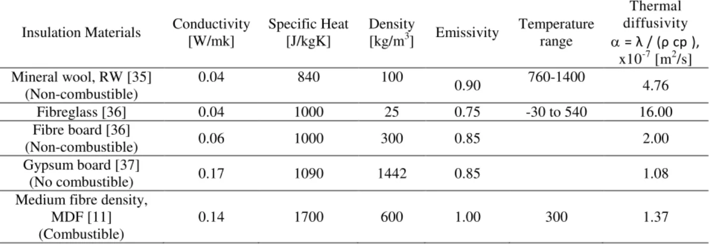
In our study, MDF and RW will be applied in the wooden slab to verify the increased resistance to insulation considering the material properties in table 6.

Table 6: Overview of the insulation material properties.

Insulation Materials Conductivity _[W/mk] Specific Heat _[J/kgK] Density _[kg/m3_] Emissivity Temperature _range

Thermal diffusivity

= λ / (ρ cp ),

x10-7 [m2/s] Mineral wool, RW [35]

(Non-combustible)

0.04 840 100 _0.90 760-1400 _4.76

Fibreglass [36] 0.04 1000 25 0.75 -30 to 540 16.00

Fibre board [36]

(Non-combustible) 0.06 1000 300 0.85 2.00

Gypsum board [37]

(No combustible) 0.17 1090 1442 0.85 1.08

Medium fibre density, MDF [11] (Combustible)

29

3.4

Thermal properties of air

The air is a mixture of different gases, mainly nitrogen and oxygen, but it contains much smaller amounts of water vapour, argon, carbon dioxide, and very small amounts of other gases. Air also contains spores, suspended dust and bacteria. Because of the wind action, the composition of air varies only a little with altitude and location, [38]. The thermal properties of air are given from the table 7. The air properties will be considered in our study, in the wooden slab with cavities and insulation material.

Table 7: Thermal properties of air, [39].

Temperature Density [kg/m3_{] Specific heat [J/kgK] Thermal conductivity [W/mk]}

20 1.166 1000 0.0258

30 1.127 1000 0.0265

40 1.091 1000 0.0272

50 1.057 1000 0.0279

60 1.026 1001 0.0299

70 0.996 1001 0.0292

80 0.967 1001 0.0299

90 0.941 1001 0.0306

100 0.916 1001 0.0312

120 0.869 1001 0.0324

140 0.827 1002 0.0349

160 0.789 1002 0.0349

180 0.754 1002 0.0362

200 0.722 1003 0.0374

250 0.6530 1003 0.0406

300 0.5960 1005 0.0437

350 0.5482 1006 0.0464

30

Chapter 4

31

4

Finite Element Method

4.1

Introduction

The finite element method is a numerical technique used to solve various problems which are attached by partial differential equations or can be formulated as functional minimization. A domain of interest is represented as an assembly of finite elements. Approximating functions in the finite elements are given in terms of nodal values of a physical field which is required. A continuous physical problem is transformed into a discretized finite element problem with unknown nodal values. For a linear problem a system of linear algebraic equations should be solved. Values inside finite elements can be recovered using nodal values, [40].

In this work, Ansys program will be used, as a finite element method, normally used to solve structural analysis, fluid dynamics, explicit and implicit methods and heat transfer. According to the numerical simulations, the thermal analysis will be used including the non-linear behaviour of the materials and the transient heat effect.

4.2

Equations and boundary conditions

For an isotropic body with temperature dependent, it is necessary to understand the heat transfer processes. In order to know the distribution of temperature in structural elements, the heat transfer is given by a basic equation as the following appearance:

t T C Q z T z y T y x T

x p 

                                   _{   } (18)

Where λ is the thermal conductivity, Cpis the specific heat of the material, ρ is the specific mass of the material, and T is the temperature field and t the time.

32 thermal energy stored within this volume. For this, it is necessary to solve the problem using the initial and their boundaries conditions [26], shown in Figure 17.

Figure 17- Boundary conditions for thermal problems in the field Ω, [41].

With the equation 18 it is possible to point out the thermal diffusivity  which determines the temperature distribution in non-steady or transient conditions, given by equation 19. In heat transfer analysis, the thermal diffusivity is the conductivity divided by the density and the specific heat.

 = λ/ (ρ Cp ) (19)

Thermal diffusivity measures the ability of a material to transmit a thermal disturbance or to conduct thermal energy relative to its ability to store thermal energy. It indicates how quickly the temperature in the material changes. Substances with high thermal diffusivity rapidly adjust their temperature to that of their surroundings, because they conduct heat quickly in comparison to their volumetric heat capacity.

33

K(λ)(T,t)(t)+ C(Cp, ρ)*(t) = F(T,t) (Q,q,hcr,Tp) (20)

F T C

KT 



(21)

Each term of the equation 21 could be represented in terms of the following expressions:





_



e N N d h N N d

K 1 1 (22)



lm e c N N d

C 1 (23)







l N Qd N qd N h d

F _e h e q e 1 1 1

 ₍₂₄₎

Where E is the total number of elements, Q is the number of elements with boundary type q,

H is the number of elements with boundary type _c and/or _r, Nl and Nm are typical shape

functions.

In the present work for two dimensional analyses an element with eight nodes and with parabolic shape functions will be used. For three dimensional analyses, linear shape functions will be used, due the solid element choosed, with eight nodes.

Using a finite difference technique to discretize the time, the system of ordinary differential equations (21) results in the recurrence formula, [42]:

 

  

 n  n

n T F

Kˆ ˆ 0  1 (25)

where

K_n K_n C_n

t

  _ 

1

 (26)

n n n n t     _ 

 F  _ C

34 Having solved the system of equations (25) forTn_, at timetn, the value of T at the

end of the time intervalt, that is, at time t_n1 is given by

n n

n T T

T            _  _ 1 1 1

1 (28)

The value of the parameter  could varies using the Crank-Nicolson scheme with

1 2, using the Galerkin scheme with 2 3 and using the Euler Backward scheme for

1.

In non-linear problems, where the thermal properties of the material are temperature dependent, the system of equations (21) can generally be written as:

) , ( ) ( ) , ( ) ( ) ,

(T t T t C T t Tt F T t

K  



(29)

There is not a general method to solve this system of non-linear differential equations. However, several numerical solution procedures, in essence, based on linear time integration and an iterative process are available, [42], [16]. In general, an effective algorithm for the analysis of non-linear transient thermal problem is used. The matrices K and C and the vector F, can vary throughout the time interval t as functions of the unknown vector temperature T

or T and time t. Therefore, these matrices must be evaluated at time t_n and the temperature

Tn+.

In order to fully satisfy these non-linear conditions of the problem, it is necessary to employ an iterative procedure in each time step. In this algorithm a modified Newton-Raphson method is used. During any step, i, of the iterative process of solution, the equation

will not generally be satisfied unless convergence has occurred. Therefore a system of residual forces  will exist:

0

ˆ

ˆ _ 1 _

 

  

 ni

i n i

n i

n  F  K T 

ψ (30)

The improved value of 1

 i n 

35

TOL

i n i n

 

  

1

 

T T

(31)

Where: TOL is the specified tolerance equal to 0.001 used in ANSYS© program,  denotes

the Euclidean vector norm, i n

T is the temperature change in the ith iteration and 1

 i n 

T is the current temperature value.

4.3

Finite elements

The finite element method is very used for the approximation of the numerical solutions for differential equations. By this "reason", a finite element formulation must be carried out using a system of algebraic equations, as is the case of the finite element program used in this work.

The finite element Plane77 with 8 nodes is used for 2D, with one degree of freedom, temperature, at each node, figure 18. The element is applicable for thermal and nonlinear material in transient analysis, [43].

Figure 18- PLANE77 geometry, [43].

36 Figure 19- SOLID90 3-D 20-Node Thermal Solid [43].

4.3.1 Shape functions for 8 nodes (Lagrange)

Quadratic two-dimensional isoparametric finite elements are presented in Figure 18. Shape functions Ni are defined in local coordinates ξ, η (−1 ≤ ξ, η ≤ 1), [40]. The term

”isoparametric” means that geometry and temperature field are specified in parametric form and are interpolated with the same functions. Both coordinates and temperature are interpolated with the same shape functions, [40].

Shape functions for 8 nodes are presented in the following: For i= I, J,K, L:























0 0

2 0

0 1 1

4 1 1

1 4 1 1

1 4

1 _{       }



i

N (32)

For i= M, O:









2 ₁

1 2 1



 

 

i

N (33)

For i= P, N:





0)1

1 ( 2

1 _{ }



i

37

In the above equations the following notation is used: ξ0 = ξξi, η0 = ηηi where ξi, ηi are

values of local coordinates ξ, η at nodes.

4.3.2 Shape functions for 20 nodes (Serendipity)

Hexahedral (or brick-type) linear 8-node and quadratic 20-node three-dimensional isoparametric elements are depicted in figure 19. Shape functions used for interpolation are

polynomials of the local coordinates ξ, η and ζ (−1 ≤ ξ, η, ζ ≤ 1).

The shape functions of the 20-node hexahedron can be grouped as follows. For the corner nodes i = I, J, K, L, M, N, O, P:

)

(e

I

N =











8

1 _{     }

i i i i i

i     

 (35)

For the midside nodes i = Q, S, U, W:











e I

N  1 1 1

4

1 2

) (

(36)

For the midside nodes i = R, T ,V, X:











e I

N  1 1 1

4

1 ₂

)

( ₍₃₇₎

38











e I

N  1 1 1

4

1 2

)

( ₍₃₈₎

39

Chapter 5

40

5

Cellular Slab With Perforations

5.1

Introduction

The wooden slabs are structural elements with increasing use in the rehabilitation of structures. For some spaces sound insulation is a key requirement like, restaurants, schools, and wood material present this characteristic. Perforations and cellular wooden slabs drew attention of experts, due their architecture, light weight, services installation and also an easy maintenance.

The construction system of the cellular slab is based on a combination of a wood panel for floor and ceiling structures, disassociated by beams, as represented in figure 20. Combining quality materials with good technique construction allow to obtains solutions as a pleasant an aesthetic lightness and safety for use. Also boards cells with slight perforations are easy to come up with great architectural features, thermal and acoustic conditions, [27].

Figure 20- Constructive models of wooden slabs, [27].

5.2

Dimensions of the perforated wooden slab

41 of each slab considers three different cellular zones (two cells with different perforations and one cell with no perforation), [11], represented in figure 21.

Figure 21- Wooden slab with cellular zones, [14].

The slabs present in the exposed surface two types of rectangular perforations (250x20) [mm] in cell 3, and (50_{× 20}) [mm] in cell 1. Other slabs present circular perforations with a diameter equal to 20[mm] in cell 3, and 10[mm] in cell 1

5.3

2D cellular slab with perforations

5.3.1 Presentation of models and geometry

In this work only the two-dimensional (2D) slab cross-sections with perforations were considered for analysis, as the previous slab dimensions. The cross-section includes three different cellular zones (two with perforations and one without perforations).

Figure 22 represents all technical drawing of the models with all considered dimensions. Autocad was the program chosen to represent and produces all these drawings.

42 Figure 22- a) Wooden cellular slab: rectangular perforation.

Figure22- b) Wooden cellular slab: rectangular perforation with 36 mm of (MDF), (RW).

Figure22- c) Wooden cellular slab: circular perforation.

3' 2' 2 Wood 3 1' 1 229 106 42

229 27 27

870 252 1150 6xR20 64 59 32 229 140 42 Insulation 106 3 6xR20 Wood 2'' 1' 2' 870 1'' 1150 3' 1 2 3'' 229 64 229 140 36 229 32 59 252 27 27 2'

1 2 3' 3

43 Figure22- d) Wooden cellular slab: circular perforation with 36mm of (MDF), (RW).

Figure22- e) Wooden cellular slab: rectangular perforation with 18mm of (MDF), (RW).

Figure22- f) Wooden cellular slab: circular perforation with 18mm of (MDF),(RW).

The nonlinear transient numerical analysis was carried out to 1800[s] according to the experimental fire exposure

Wood 2' 3 1 2'' Insulation 1' 3' 2 1'' 3'' 229 252 104 32 4xD20 23 229 140 104 59 8xD10 27 10 64 870 27 1150 36 229 229 27 870 3' Wood 1' 32 2' 27 18 252 2'' 229

1 2 3

229 64 140 1'' 1150 106 6xR20 42 59 Insulation 3'' 1'' 3'' 2 1' 3 Wood 3' Insulation 2'' 2' 1 229 59 1150 140 104 4xD20 64

10 23 252

44 For this work different numerical models were defined as represented in table 8.

Models 1 to 6 consider the applied ISO 834 standard fire at the perforated bottom surface .These models will be implemented and compared with the models 7 to 12, where the

exposure fire ‘’Furnace’’ as the same behaviour like in the experimental tests in laboratory

[14]. The main goal was to simulate in 2D analysis the same occurrence as in 3D experimental. Models 7 and 9 permit to conclude about the use of the 2D model as an alternative when compared with the same behaviour in 3D experimental tests.

Also, other numerical comparison will be produced between models with the typical

boundary condition ‘’Furnace’’ and the ISO 834 fire, due the new introduction of the insulation material effect in wood material, with different applied external conditions. According to this, all the remaining and more additional 2D models could be used with more performance and with different proposal (different insulation materials and board sizes) to obtain different conclusions for building wooden slab applications.

Table 8: Numerical models characterizations.

Models Number of Figures Geometrics Boundary Conditions

Model 1 Figure 22.a) Rectangular

ISO 834

Model 2 Figure 22.b)

Rectangular with MDF=36mm Rectangular with MDF=36 mm, internal air

Rectangular with RW=36mm Rectangular with RW=36mm, internal air

Model 3 Figure 22.c) Circular

Model 4 Figure 22.d)

Circular with MDF=36mm Circular with MDF=36mm, internal air

Circular with RW=36mm, internal air

Model 5 Figure 22.e)

Rectangular with MDF=18mm Rectangular with MDF=18mm, internal air

Rectangular with RW=18mm, internal air

Model 6 Figure 22.f)

Circular with MDF=18mm Circular with MDF=18mm, internal air Circular with MDF=18mm, internal air

Model 7 Figure 22.a) Rectangular

Furnace

Model 8 Figure 22.b) Rectangular with 36 mm of MDF

Model 9 Figure 22.c) Circular

Model 10 Figure 22.d) Circular with 36 mm of MDF

Model 11 Figure 22.e) Rectangular with 18 mm of MDF

45

5.3.2 Mesh and boundary conditions

A 2D finite element (Plane77) with 8 nodes was used for thermal and nonlinear material in transient analysis, using ANSYS© program. In order to fully satisfy the nonlinear conditions of the numerical problem, an iterative procedure in each time step it is necessary to apply. Figure 23 presents the correspondent mesh used in some models.

Model 1 / 7 Model 3 / 9

Model 2 / 8 Model 4 / 10

Figure 23- Mesh of finite element, plane77.

In ANSYS©, a modified Newton-Raphson method was adopted to solve the nonlinear problem, and the time interval considered for each step was equal to 10[s] and the minimum time equal to 0.1[s]. The bottom surface of the wooden slab was exposed to the boundary conditions according table 8 during 1800[s].

In wooden slabs without insulation material, the temperature on the internal cavities follows real heating curves obtained during the previous experimental tests, [27], [30], and measured with plate thermocouples. Figure 24 shows the values of each curve applied according the cell (TP1, TP2, TP3) and according the perforation type (rectangle or circle).

The convection coefficient is considered equal to 25[W/m2K] [16] inside cavities and in the exposed fire surface. At the unexposed surface the room temperature is equal to 20[ºC] and the convection coefficient is equal to 4[W/m2K]. The emissivity of the flames is taken equal to 1 for exposed side and internal cavities [16] and 0.8 for timber, according to Eurocode 5, [15]. The model with insulation material, all the adjacent cellular zones was filled with internal air, and only the conduction effect was considered.

46 curves were used in the numerical simulations. The ‘’Furnace’’ curve represents the increase temperature and the cooling effect during all experimental tests. This curve is more energetic due the conditions imposed by the space volumetric furnace and also due the wood material combustion.

Figure 24- Temperature curves used inside the cavities in numerical analysis.

Figure 25- Curves of fire exposure ‘’Furnace’’ and ISO 834. 0

100 200 300 400 500

0 200 400 600 800 1000 1200 1400 1600 1800

T

empera

ture

, º

C

Time, s

Small_rectangular_TP1 Without_rectangular_TP2 Large_rectangular_TP3 Small_circular_TP1 Without_circular_TP2 Large_circular_TP3

0 200 400 600 800 1000 1200

0 200 400 600 800 1000 1200 1400 1600 1800

T

empera

ture

, º

C

Time, s

47

5.3.3 Results of 2D models

5.3.3.1 Charring rate

For the calculation of the charring rate by the numerical method, the criterion adopted was to calculated the isothermal at 300[ºC], determining the time instant that occurrence and calculate the developed char layer for each model.

The temperature limit at which it is estimated that the timber is completely carbonized is 300[°C], [15]. The timber which is at a temperature above this value is fully carbonized, below this temperature the wood is still intact. Firstly, it is necessary to know the value of the char layer for each model. The table below shows the thickness of char layer for each model with the considered time instant.

Table 9: Char layer depth.

Models Time (s) Cell 1 [mm] Time (s) Cell 2 [mm] Time (s) Cell 3 [mm]

Model 1 604.752 9 604.752 8 604.752 9

Model 2 630.062 9 716.663 8 630.062 9

Model 3 -- -- 774.732 9 389.732 9

Model 4 -- -- 784.967 9 404.967 9

Model 5 640 9 770 8 640 9

Model 6 -- -- 784.586 9 399.586 9

Model 7 286.972 9 331.97 9 286.972 9

Model 8 300.428 9 330.428 8 300.428 9

Model 9 -- -- 320.809 9 -- --

Model 10 -- -- 300.862 8 230.699 8

Model 11 292.622 9 327.662 9 292.662 9

Model 12 -- -- 332.427 9 -- --

48 For circular models with and without MDF only the charring rate in cell 2 and cell 3 in some models were calculated. For cell 1 the perforations are totally charred at this time instant and for this reason it was not calculated.

There are typical design values for charring rate of wood between 0.5-1.0[mm/min]. Eurocode 5 [15] suggests a charring rate equal to 0.65[mm/min] for solid wood with density greater than 290[kg/m3]. The evaluation of the char layer thickness depends on the exposed time and determines the charring rate in mm/min, shown in the table 10. The values are approximately equal to the reference value of EC 5 part 1.2, [15]. Cell 2 in all tested wooden slabs has a mean value equal to 0.71mm/min. On the other hand, in cell 1 and 3, the charring rates values are higher, due to perforations and their round effect. For models with ‘’Furnace’’ the results were compared with the results obtained previously from David and Meireles, [27], [30]. The numerical results obtained showed that the value of charring rate reaches more than 1 [mm/min], as the same results obtained from David and Meireles, [27], [30].

Table 10: Charring rates values.

Charring rate [mm/min]

Models Cell 1 Cell 2 Cell 3

Model 1 0.89 0.79 0.89

Model 2 1.04 0.67 1.04

Model 3 -- 0.69 1.38

Model 4 -- 0.68 1.33

Model 5 0.84 0.75 0.84

Model 6 -- 0.68 1.35

Model 7 1.88 1.62 1.88

Model 8 1.8 1.63 1.80

Model 9 -- 1.68 --

Model 10 -- 1.59 2.08

Model 11 1.84 1.63 1.84