Dynamic Analysis of Numerical Mesoscale Models of Composite Materials

André Alves Silva

Licenciado em Ciências de Engenharia Mecânica

Dynamic Analysis of Numerical

Mesoscale Models of Composite

Materials

Dissertação para obtenção do Grau de Mestre em Engenharia Mecânica

Orientadora: Professora Doutora Marta Isabel Pimenta

Verdete da Silva Carvalho, Professora Auxiliar Convidada da

Faculdade de Ciências e Tecnologia da Universidade Nova de

Lisboa

Co-Orientador: Doutor Pedro Miguel de Almeida Talaia,

Engenheiro de I&D, CEiiA

Júri:

Presidente: Doutor Pedro Samuel Gonçalves Coelho Arguente: Doutor João Mário Burguete Botelho Cardoso Arguente: Doutor Bernardo Rodrigues de Sousa Ribeiro Vogal: Doutor Pedro Miguel de Almeida Talaia

Dynamic Analysis of Numerical Mesoscale Models of Composite Materials

Copyright  2016 André Alves Silva

Faculdade de Ciências e Tecnologia da Universidade Nova de Lisboa

A Faculdade de Ciências e Tecnologia e a Universidade Nova de Lisboa têm o direito, perpétuo e sem limites geográficos de arquivar e publicar esta dissertação através de exemplares

impressos reproduzidos em papel ou de forma digital, ou por qualquer outro meio conhecido ou que venha a ser inventado, e de a divulgar através de repositórios científicos e de admitir a sua

i

Acknowledgements

To Assistent Professor Marta Carvalho, supervisor of this dissertation, for her availability to help

me, and the patience and encouragement provided in the most difficult times. For all she taught me, even in times I was more nervous she always helped me.

To Assistent Professor João Cardoso, for all he taught me throughout my academic life and for his availability to help me in times of need.

To Faculdade de Ciências e Tecnologia at Universidade Nova de Lisboa and CEiiA for the opportunity to develop this dissertation, and more particularly, to Dr. Pedro Miguel de Almeida Talaia for all the advices he gave me, even in the most occupied times.

To all the professors of the Department of Mechanical and Industrial Engineering, for all their contribution to my academic career.

To my family, who never stopped supporting and helping me. To my mother and my father, my pillars, who helped me in the moments I needed the most.

To Dr. Carla Machado for all the support and help she gave me.

iii

Abstract

The role of composites in the industry has been increasing over the past few years. One of the main reasons for this phenomenon is due to these materials presenting the best properties of their

constituents and often qualities that neither of the constituent materials have. However, as a consequence, composite structures are becoming more complex, and its behavior more difficult to

predict.

The study of this dissertation arises from Crespo’s dissertation, and had its origin on the need to predict the behavior of composite materials specimens in a less expensive and faster manner. To

fulfill this need, a methodology was developed using LS-DYNA finite element mesoscale models.

This methodology uses an explicit dynamic analysis, and is capable of testing composite specimen models subjected to tensile and compressive loads. However, this type of analysis is different from the one Crespo used and phenomenons like hourglass must be considered. For this case study the

material model consists in a spread tow carbon fabric with0°/90°, 15°/75° and 30°/60° arrangements. To simulate the behavior of this composite material, when subjected to external loads, failure and

damage propagation such as delamination, fiber and matrix failure are implemented in the models. The failure of the matrix and the fibers are controlled by a combined failure criterion implemented

in LS-DYNA code.

Knowing only the dimensions of the test specimens, the material properties were taken from Crespo’s

dissertation. To validate the models, results were compared with Mangualde’s, whose methodology was developed using an implicit static analysis.

v

Resumo

O papel dos materiais compósitos na indústria tem vindo a aumentar ao longo dos últimos anos. Uma

das principais razões para este fenómeno deve-se ao facto destes materiais apresentarem propriedades superiores ao dos seus constituintes e, na maior parte das vezes, qualidades que nenhum

dos materiais constituintes tem. No entanto, como consequência, as estruturas de compósitos são cada vez mais complexas e o seu comportamento cada vez mais difícil de prever.

O estudo feito nesta dissertação surge no âmbito da dissertação da Inês Crespo, e teve a sua origem na necessidade de prever o comportamento de provetes de materiais compósitos de uma forma menos dispendiosa e mais rápida. A fim de cumprir esta necessidade, foi desenvolvida uma metodologia

com recurso a modelos à meso-escala de elementos finitos utilizando o LS-DYNA.

Esta metodologia utiliza uma análise dinâmica explícita e é capaz de testar modelos de amostras de

compósitos submetidos a cargas de tração ou compressão. No entanto, este tipo de análise é diferente da que a Inês Crespo utilizou e fenómenos como o hourglass têm de ser considerados. Para este

estudo o material consiste num tecido ultrafino de carbono com fibras orientadas a 0°/90°, 15°/75° e 30°/60°. De forma a simular o comportamento deste material quando submetido a cargas externas,

foram implementados mecanismos de falha e propagação de dano no modelo, tais como delaminação e falha das fibras e da matriz. Estas últimas são controladas por uma combinação de dois critérios de

falha que se encontram implementados no código do LS-DYNA.

As propriedades dos materiais foram obtidas do modelo numérico da dissertação de Inês Crespo, conhecendo-se apenas as dimensões dos provetes. De forma a validar a metodologia, os resultados

apresentados nesta dissertação foram comparados com os resultados obtidos por Pedro Mangualde, cuja metodologia foi desenvolvida recorrendo a uma análise estática implícita.

Palavras-Chave:

vii

Table of Contents

1

Introduction ... 1

1.1 Motivation ...1

1.2 Objectives ...2

1.3 Structure ...3

2

Theoretical Framework ... 5

2.1 Concepts of Composite Materials ...5

2.1.1 Reinforcement ... 6

2.1.2 Matrix ... 7

2.1.3 Textile Composites ... 7

2.2 Constitutive Law’s for Composite Materials ...10

2.2.1 Hooke’s Law ... 11

2.3 Multi-scale Models...12

2.3.1 Microscale Models ... 13

2.3.2 Mesoscale Models... 14

2.3.3 Macroscale Models ... 14

2.4 Damage in Composite Materials ...14

2.4.1 Failure Modes ... 15

2.4.2 Failure Criteria ... 19

2.5 Testing and Certification ...22

2.6 Dynamic Analysis – General Considerations ...24

2.7 Hourglass Control ...26

3

Numerical Analysis

–

Model Testing ... 29

3.1 Delamination ...29

3.1.1 Delamination Analysis and Results ... 32

3.2 Combined Failure Criterion ...37

3.2.1 Implementation of the Combined Failure Criterion in LS-DYNA ... 38

viii

4

Numerical Analysis of Models of CFRP Test Specimens ... 45

4.1 Numerical model of a test specimen with a 0°/90° arrangement ...46

4.2 Numerical model of a test specimen with a 15°/-75° arrangement ...50

4.3 Numerical model of a test specimen with a 30°/-60° arrangement ...53

4.4 Numerical model of a test specimen constituted by 10 plies with a 0°/90° arrangement ...56

4.5 Numerical model of a compression test specimen constituted by 26 plies with a 0°/90° arrangement ...59

4.6 Conclusion Remarks ...63

5

Conclusion and Future Works ... 65

References... 67

ix

List of Figures

Figure 1.1- Experimental results of a test specimen constituted by 26 plies with four different

orientations and an organizational chart describing the work that will be developed ... 2

Figure 2.1-Different types of reinforcements [7] ... 6

Figure 2.2-Representation of the different types of woven fabrics [9] ... 8

Figure 2.3 - Sample of a spread-tow carbon fabric [11] ... 9

Figure 2.4 - Comparison between a conventional woven fabric and a spread-tow fabric [12] ... 9

Figure 2.5- Typical behavior shown by isotropic, anisotropic and orthotropic material subjected to axial tension [6] ... 10

Figure 2.6- Unidirectional composite material constituted by the fiber and matrix [14] ... 11

Figure 2.7-The different models at different scales [18] ... 12

Figure 2.8- Representation of the three different scales and their respective features [20] ... 13

Figure 2.9- Fracture surfaces for each state of stress and the four main failure modes [23] ... 16

Figure 2.10- Usual kink band geometry [25] ... 18

Figure 2.11- The building-block approach represented in a pyramid [1] ... 23

Figure 2.12- Demonstration of the deformation of an element with reduced integration when subjected to a bending load [35] ... 27

Figure 3.1-Three modes of delamination fracture [1] ... 29

Figure 3.2-Mixed mode traction-separation law [37] ... 30

Figure 3.3 - Schematic of interface elements [39] ... 32

Figure 3.4 - DCB specimen [41] ... 32

Figure 3.5 - Test specimen modeled in LS-DYNA ... 33

Figure 3.6 - Test specimen after delamination – VM Stress [Pa] ... 35

Figure 3.7 - Load-Displacement curves - comparison between LS-DYNA simulations and experimental data ... 36

Figure 3.8 - Load-Displacement curves - comparison between LS-DYNA and ANSYS numerical simulations and experimental data ... 36

Figure 3.9 - Combination of the maximum stress (represented in black) and the Tsai-Wu (represented in blue) failure criteria [2] ... 38

Figure 3.10 - Test speciment generated by the Mesh generation algorithm... 40

Figure 3.11 - Test specimen with respetive boundary conditions ... 41

Figure 3.12 – Damage propagation of the test specimen ... 41

Figure 3.13 - Illustration of all the failed elements of the 0º ply ... 42

x

Figure 3.15 - Damage propagation of Mangualde's test specimen ... 43

Figure 3.16 - Comparison between the Force vs Displacement curves obtain in ANSYS and LS-DYNA ... 44

Figure 4.1- Representation of the test specimen with 0°/90° arrangement and respective boundary conditions ... 46

Figure 4.2- Final stage for the test specimen with 0°/90° arrangement with cohesive contact ... 48

Figure 4.3- Final stage for the test specimen with 0°/90° arrangement without cohesive contact ... 48

Figure 4.4- Comparison between the Force vs Displacement curves for both 0°/90° models ... 49

Figure 4.5- Comparison between the results obtained in LS-DYNA and ANSYS for the 0º/90º model ... 50

Figure 4.6 - Test specimen with a 15º/-75º arrangement ... 51

Figure 4.7- Final stage for the test specimen with 15°/-75° arrangement with cohesive contact .... 51

Figure 4.8- Final stage for the test specimen with 15°/-75° arrangement without cohesive contact 51 Figure 4.9- Comparison between the Force vs Displacement curves for both 15°/-75° models ... 52

Figure 4.10- Comparison between the results obtained in LS-DYNA and ANSYS for the 15º/-75º numerical model ... 53

Figure 4.11- Test specimen with 30°/-60° arrangement ... 54

Figure 4.12- Final stage for the 30°/-60° test specimen with cohesive contact ... 54

Figure 4.13- Final stage for the 30°/-60° test specimen without cohesive contact ... 54

Figure 4.14- Comparison between the Force vs Displacement curves for both 30°/-60° models .... 55

Figure 4.15- Comparison between the results obtained in LS-DYNA and ANSYS for the 30º/-60º numerical model ... 56

Figure 4.16- Representation of the test specimen constituted by 10 plies ... 57

Figure 4.17- Final stage for the test specimen of 10 plies with cohesive contact ... 58

Figure 4.18- Final stage for the test specimen of 10 plies without cohesive contact ... 58

Figure 4.19- Comparison between the Force vs Displacement curves for both models of 10 plies 58 Figure 4.20 - Representation of the test specimen constituted by 26 plies ... 59

Figure 4.21 - Final stage for the test specimen of 26 plies without a constrain in the y-direction ... 61

Figure 4.22 - Final stage for the test specimen of 26 plies with a constrain in the y-direction ... 61

xi

List of Tables

Table 2.1- Hourglass control for each element type ... 28

Table 3.1 - Dimensions of the test specimen... 34

Table 3.2 - Material properties of the plies and the cohesive elements taken from [40] ... 34

Table 3.3 - Final properties of the material of the cohesive elements ... 35

Table 3.4 - Dimensions of the spread tow carbon fabric ply... 40

Table 3.5 - Material properties of the spread tow carbon fabric ply [46] ... 40

Table 3.6 - Failure tensions provided by the five uniaxial tests [1,21] ... 40

Table 4.1- Properties for the cohesive contact taken from [46] ... 47

Table 4.2- Relation between the input variables of the cohesive contact option 9 and the material *MAT_138 ... 47

Table 4.3- Dimensions of the test specimen of 10 plies ... 57

Table 4.4 - Dimensions of the test specimen of 26 plies ... 60

Table 4.5 - Material properties of the plies ... 60

Table 4.6 - Properties of the cohesive contact/element ... 60

Table 4.7 – Value of the failure tensions ... 61

xiii

Nomenclature and List of Symbols

CFRP Carbon Fiber Reinforced Polymer

RTM Resin transfer molding

SRIM Structural reaction injection molding

RFI Resin film infusion

FEM Finite element method

RVE Representative volume element

HG Hourglass

S/R Selectively reduced

CPE Cosserat Point Element

IFT Interlaminar fracture toughness

VCCT Virtual crack closure technique

TBI Tie-Break interface

CZM Cohesive zone model

DCB Double cantilever beam

𝜎 Stress

𝜀 Strain

𝐸𝑖 Young’s moduli for the i-direction

𝑣𝑖𝑗 Poisson’s ratio

𝐺𝑖𝑗 Shear moduli for the plane ij

𝑋𝑇 Failure stress under longitudinal tension

𝑋𝐶 Failure stress under longitudinal compression

𝑌𝑇 Failure stress under transversal tension

𝑌𝐶 Failure stress under transversal compression

𝑆𝐿 Failure stress under pure shear

𝛼 Fracture angle

𝜀𝑖𝑇𝑢 Tensile normal failure strain

𝜀𝑖𝐶𝑢 Compressive normal failure strain

𝜀_𝑖𝑗𝑇𝑢 _{Shear strain failure in the plane ij}

𝐹𝑖𝑗 Variables implemented in the Tsai-Wu failure criterion

xiv

𝜋 Kinetic energy

𝑢 displacement

𝑢̇ Velocity

𝑀𝐽𝐾 Mass matrix

𝐶𝐽𝐾 Damping matrix

𝐾𝐽𝐾 Stiffness matrix

𝑢̅𝑘 Amplitude of the sinusoidal vibration

𝑤 Natural frequency

𝐺𝐼𝐶 Critical energy for Mode I

𝐺𝐼𝐼𝐶 Critical energy for Mode II

𝐺𝐼𝐼𝐼𝐶 Critical energy for Mode III

𝐸𝑁 Stiffness normal to the plane of the cohesive element

𝐸𝑇 Stiffness in the plane of the cohesive element

𝛿𝑚 Mixed-mode relative displacement

𝛿𝐼 Separation in the normal direction for Mode I

𝛿𝐼𝐼 Separation in the transverse direction for Mode II XMU Exponent of the mixed mode criteria

𝛿𝐹 The ultimate mixed-mode displacement

𝛽 “mode mixity”

𝑊 Width

𝐿 Length

𝑡 Thickness

𝑇1 Peak traction in the normal direction

𝑆 Peak traction in the tangential direction

𝐾 Interface stiffness

𝑈𝑁𝐷 The ultimate displacement in the normal direction

Chapter 1 – Introduction 1

1

Introduction

1.1

Motivation

Composites materials have existed for a long time, however their importance has been increasing over the past few years. In the automobile, aeronautic and naval industry the use of these materials

is becoming higher, replacing the use of traditional materials. As a consequence, the requirements are becoming more specific and the composite structures more complex. For this reason, it is very

important and a priority for an engineer the knowledge and comprehension of the characteristics and behavior of these materials.

As technology evolves, new ways of producing composites are being developed. Currently, carbon fiber reinforced polymer (CFRP) is a new composite material that is being introduced in the industry. The properties and behavior of this composite are acquired by very expensive tests using the Building

Block approach [1]. These new materials can be characterized by their matrix, which can be, for example, an epoxy resin, their reinforcement material and stacking sequence (number, thickness and

fiber orientation). It is important to note that a single change in the characteristics of these materials would imply a repetition of the tests previously submitted.

The present dissertation follows on Crespo’s dissertation [2], that developed numerical mesoscale models for static analysis of composite materials in order to study its collapse when subjected to

uniaxial compression tests. Some factors were identified in order to improve the work that Crespo developed, including the computational cost and parameter identification using optimization

methodologies. With this under consideration, it was proposed the development of numerical models for dynamic analysis that, not completely replacing the experimental tests that are already

2 Chapter 1 – Introduction

1.2

Objectives

As previously stated, nowadays the knowledge of composite material structures are acquired using

the Building Block approach, which will be described further ahead. However, the cost and time inherent to this approach becomes counter-productive. Due to that, the development of numerical models is becoming an increasingly important tool, allowing most of the knowledge to be acquired

in a faster and less expensive way.

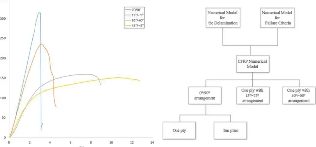
In this dissertation, in order to develop a numerical model for predicting composite material behavior capable of providing accurate results it is required to establish objectives. The main objective of this dissertation is to develop numerical mesoscale models for explicit dynamic analysis with different

arrangements using LS-DYNA [3] and respectively validate them with Mangualde’s models [4], whose dissertation was developed in the same semester, and the results obtained from experimental

tests. In Figure 1.1 an example of experimental results obtained from testing test specimens constituted by 26 plies subjected to compressive loads is represented as well as an organizational

chart describing the work that will be developed in a structured way.

Figure 1.1- Experimental results of a test specimen constituted by 26 plies with four different orientations

Chapter 1 – Introduction 3

1.3

Structure

The work that was developed and described in the present dissertation is divided in five chapters,

being this chapter the first, where the motivation, objectives and the respective structure are described.

In Chapter 2 is presented the state of the art, where the theoretical concepts are described. In this

chapter, most of the work and studies that have been done related to composite materials, multiscale

modes, failure modes, failure criteria and dynamic analysis, among other relevant subjects, are presented.

In Chapter 3 a detailed review of delamination, the combined failure criteria and their respective

implementations in the LS-DYNA code are presented. The respective models are then described and simulated, comparing the results with the ones obtained by Mangualde’s simulation, and respectively

validated.

Chapter 4 is presented as the final chapter of results, where ten numerical modes, six models of one

ply with a 0°/90°, 15°/-75° and 30°/-60° arrangement, with and without cohesive contact and two models for ten and twenty-six plies with a 0°/90° arrangement are tested implementing all the features

described in the previous chapters. The results are then compared with the results obtained by Mangualde and Crespo’s simulation.

Finally, in chapter five all the conclusions obtained during all the work that was developed throughout this dissertation are presented, as well as a review of the objectives that were proposed in the beginning. In the last subject of this chapter, ideas and improvements are suggested in order to

Chapter 2 – Theoretical Framework 5

2

Theoretical

Framework

2.1

Concepts of Composite Materials

A composite material can be defined as a combination of two or more distinct materials in a

macroscopic structural unit, having a recognizable interface between them [2,5].

Given the information in the ASM Handbook Vol. 21 [1], composites are commonly classified at

two distinct levels. The first level refers to the matrix constituent, in which these materials act as a binder for the reinforcements, transferring the loads between and protecting them from the environment. The second level refers to the reinforcement constituent. It is the reinforcement which

gives the composite its desired properties. Composites can also be classified by a continuous phase (the matrix) and a discontinuous phase (the reinforcement). As stated by George H. Staab [6] the

constituents are generally arranged so that one or more discontinuous phases are embedded in a continuous phase.

The resulting composite has a superior balance of structural properties comparing to either constituent material alone. This balance and, as a consequence, improved structural properties, result

from a load-sharing mechanism.

A material is generally stronger and stiffer in fiber form than in bulk form. Individual fibers are

harder to control and arrange in usable components. Therefore a binder material (the matrix) is required and must be continuous in order to surround each fiber so that they are kept distinctly

separate from adjacent fibers, allowing the entire material system to be easier to handle and work with [6].

6 Chapter 2 – Theoretical Framework The main advantage of these materials is that they usually present the best properties of their constituents and often qualities that neither of the constituent materials have [2]. Some of the

properties that can be improved by producing a composite material are strength, stiffness, corrosion resistance, wear resistance, weight, fatigue life, temperature-dependent behavior, thermal insulation,

thermal conductivity or acoustical isolation [2].

2.1.1

Reinforcement

As previously stated, the reinforced constituent is the component that provides the desired properties to the final product (the composite material), whether it’s strength, stiffness or both. These constituents can be classified in three different ways: particulate, continuous and discontinuous

fibers, as represented in Figure 2.1. Reinforcement is considered to be a “particle” if all of its dimensions are roughly equal [1].

According to Music and Witdroth [7], when using short fiber (particulate or discontinuous) it’s required that the matrix transfers the load between the reinforcement more frequently, resulting in a

composite with low properties when compared with a composite that is reinforced with continuous fibers.

The first composites ever produced were the fiberglass-reinforced plastics, which are sometimes

referred to as “basic” composites, but nowadays the most widely used are the advanced fibers, such

as carbon and graphite fibers [5]. The advantages of these fibers, when compared with glass fibers, are their higher modulus and lower density.

The reinforcement material of the specimens studied in this dissertation is Carbon Fiber.

Chapter 2 – Theoretical Framework 7

2.1.2

Matrix

The matrix constituents can be polymers, metals or ceramics, depending on the particular requirements [5]. It’s the matrix that holds the fibers together in a structural unit, due to their cohesive and adhesive characteristics, protecting them from external damage, as well as transferring and

distributing the applied loads to the fiber, allowing the strength of the reinforcements to be used to their full potential [3,1]. It also provides a solid form to the composite in order to facilitate handling

during manufacture. As previously stated the reinforcements are stronger and stiffer than the matrix. Therefore, as a continuous phase, the matrix controls the transverse properties, interlaminar strength

and elevated-temperature strength of the composite.

Polymers are the most widely used matrix materials and the two most common within the polymers

are epoxy resin and polyester [2], being the specimen studied here composed by an epoxy resin.

2.1.3

Textile Composites

Over time, these type of composites have gain more and more importance in modern industry and

are currently used in advanced structures in automobile, marine and aerospace industry, due to their mechanical properties, easy handle and low cost of the reinforced materials [8].

The mechanical properties of these materials are characterized by their anisotropy and inhomogeneous nature. As a consequence there are several parameters to take into account in order

to control their mechanical properties such as fiber architecture, fiber properties, matrix properties, etc [8].

These composite are manufactured by impregnating matrix materials into their dry preforms in order to hold the multidirectional yarns together, using techniques such as: RTM (resin transfer molding),

SRIM (structural reaction injection molding) and RFI (resin film infusion) [8].

Textiles composites can be distinctly separated in three structural levels: microscale, mesoscale and macroscale.

Textiles can also be classified in three different categories: woven fabrics, knitted fabrics and braided fabrics. Woven fabrics are the most widely and most commonly used in structural applications, and

8 Chapter 2 – Theoretical Framework 2.1.3.1 Woven fabrics

Woven fabrics are manufactured using the multiple warp weaving method, which consists of two

sets of interlaced yarn components (one is called warp and the other weft, according to the yarn orientation). The mostly used woven fabrics in textile composites are the 2D fundamental weaves,

for example plain, twill and satin weaves. Each one is identified by the repeating patterns of the interlaced regions in the warp and weft directions [8]. The three types of woven fabrics previously

discussed are presented in Figure 2.2.

Figure 2.2-Representation of the different types of woven fabrics [9]

2.1.3.1.1 Spread tow carbon fabric

CFRP composites presently evolving rapidly, as a result of the research and development being done

nowadays. One of the main goals is to obtain lighter composites structures, as well as improving their performance/cost ratio, which may be interpreted as significant increase in properties with no

additional cost. In order to make lighter structures, a recent method was developed called spread-tow technology. Figure 2.3 represents an example of this technology implemented in a carbon fabric. As

recent studies show [10], the use of this technology allows us to get thinner plies, which is very important due to the key role of the thickness in controlling the mechanical properties of the

Chapter 2 – Theoretical Framework 9 Figure 2.3 - Sample of a spread-tow carbon fabric [11]

This tow-spreading technology consists of passing a tow through a spreading machine that is

equipped with an air duct and a vacuum that sucks the air downward through the air duct. The use of this technology allows the production of unidirectional plies or woven fabric plies [1,8].

Figure 2.4 - Comparison between a conventional woven fabric and a spread-tow fabric [12]

2.1.3.2 Pre-peg

Pre-peg is a term for pre-impregnated composite fibers where the matrix material, such as epoxy

10 Chapter 2 – Theoretical Framework be a fabric or unidirectional, and the two main methods of producing them are: hot melt and solvent dip.

The use of these materials can provide great advantages over conventional resin deposition during final production of the composite, due to the precise control of the ratio of fiber-resin, controlling the

flow of resin during the curing process and in some processes, better control of the orientation and positioning of the fibers [1].

In this dissertation, the models consist of a spread tow carbon fabric pre-impregnated with an epoxy resin.

2.2

Constitutive Law’s for Composite Materials

Composite are very complex materials and most of them either have an anisotropic or an orthotropic

behavior.

In the case of an anisotropic material, its properties are different in all directions. These materials

can, sometimes, result from the combination of two isotropic materials, which are a materials whose properties are assumed to be uniform in all directions. For example, when given two isotropic

conducting materials, like a metal with high conductivity and a plastic that is electrically insulating, combining the two materials in alternating layers results in a highly anisotropic composite [13]. The

anisotropic behavior of a material can vary in different ways and when subjected to applied loads, the actual deformation will depend on the material [6].

As stated by George H. Staab [6] for an orthotropic material, its properties are different in three

mutually perpendicular planes. However, contrary to an anisotropic material, there is generally no shear-extension coupling. Because Poisson’s ratio is different in the in-plane and out-of-plane

directions, the respective transverse displacements are not typically the same. Figure 2.5 represents the response of an isotropic, anisotropic and orthotropic material when subjected to axial tensions.

Although the response of the orthotropic materials appears similar to the isotropic material, the magnitudes of the in-plane and out-of-plane displacements are different [6].

Figure 2.5- Typical behavior shown by isotropic, anisotropic and orthotropic material subjected to axial

Chapter 2 – Theoretical Framework 11 The fibers of the CFRP plate that are being studied in this dissertation are considered to have an

anisotropic behavior, however they can also be considered to have a transverse isotropic behavior. For a transversely isotropic material, in addition to the three planes of symmetry, there is an axis of

material symmetry. Thereby, any two material fibers having symmetrical positions with respect to the axis of symmetry have the same stiffness [6]. For example, a cell of a unidirectional composite

material can be considered as being constituted by a fiber embedded in a cylinder of matrix, resulting in a material with an orthotropic behavior, having an axis of revolution in addition, which classifies

this material as transversely isotropic, represented in Figure 2.6 [14].

Figure 2.6- Unidirectional composite material constituted by the fiber and matrix [14]

2.2.1

Hooke

’s Law

In this area, it is very important to know the relation between stress and strain. However, this relation depends on the type of material under consideration. For specimens considered to have an elastic

behavior, this relation is known as Hooke’s law.

For orthotropic materials, the compliance matrix [𝑆] is expressed in the following form [15]:

[𝑆] =

[ 1

𝐸1 −

𝑣21

𝐸2 −

𝑣31

𝐸3 0 0 0

−𝑣_𝐸12

1

1

𝐸2 −

𝑣32

𝐸3 0 0 0

−𝑣13

𝐸1 −

𝑣23

𝐸2

1

𝐸3 0 0 0

0 0 0 _𝐺1

23 0 0

0 0 0 0 _𝐺1

31 0

0 0 0 0 0 _𝐺1

12]

12 Chapter 2 – Theoretical Framework where 𝐸₁, 𝐸₂ and 𝐸₃ are Young’s moduli in directions 1, 2 and 3, respectively. 𝑣_𝑖𝑗are Poisson’s ratio

and 𝐺₂₃, 𝐺₃₁ and 𝐺₁₂ are the shear moduli in the 2-3, 3-1 and 1-2 planes, respectively.

Given the symmetry of the compliance matrix, i.e. 𝑆_𝑖𝑗= 𝑆_𝑗𝑖 [15]:

𝑣𝑖𝑗

𝐸𝑖 =

𝑣𝑗𝑖

𝐸𝑗, 𝑖, 𝑗 = 1,2,3. (2.2)

Therefore, the stress-strain relation for orthotropic linear elastic materials can be expressed as,

[𝜀] = [𝑆][𝜎]. (2.3)

2.3

Multi-scale Models

The knowledge of fiber reinforced composite materials has increased over the last decades. Due to their microscopic heterogeneity, as well as the randomness of the fiber’s positions, their bounding with the matrix and the presence of microdefects, the damage and non-uniform behavior of these

composites, when subjected to external loads, becomes very complex and hard to predict [16]. In the field of composite materials, the study of these physical phenomenons takes a huge role. Physical

phenomena can be characterized by a hierarchy of different complex models which are better suited at the appropriate scales, represented in Figure 2.7. As stated by Wan, Sun and Gu [17], “The multi

-scale models can be defined as constitutive models in which the global constitutive behavior of

composite material is determined simultaneously throughout the analysis based on the behavior of the constituents and their interactions”. These models provide a solid structure, based on fundamental principles, in order to develop mathematical and computational models of such

phenomena [18].

Chapter 2 – Theoretical Framework 13 Nowadays, when using finite element method (FEM) models to study these composites, different scales can be considered. These models can reach from micro unit cell models for crack propagation

analysis to models with complete structural part made of composite material [19]. The most common levels are: microscale, mesoscale and macroscale. The first one defines the arrangement of the fiber,

the mesoscale presents the fabric structure and fiber bundle and the macroscale works as a bounding mechanism between the unit cell and the engineering structure. Figure 2.8 represents the different

scale levels as well as their respective features [20].

Figure 2.8- Representation of the three different scales and their respective features [20]

2.3.1

Microscale Models

As stated by Zhang [20], microscale models allow the forecast of the properties of the transversely isotropic unidirectional laminate. These models are always based on a representative volume element (RVE). As previously presented in Figure 2.8, at a microscale level, the fibers are embedded in matrix

materials in order to form a yarn and a tow. The main objective of this scale is to compute the stress redistribution surrounding the broken fibers with different interfacial deformation models and, from

these tests, obtain the average stress concentrations induced around the unbroken fibers and the stress recovery throughout the broken fiber [16].

Although this approach presents a good solution in order to approximately predict the properties of the unidirectional lamina, when modelling textiles and more complex composites the resort to this

14 Chapter 2 – Theoretical Framework

2.3.2

Mesoscale Models

At the meso level, the fiber bundles are composed by micro level composites. The laminate is considered homogeneous and the material orthotropic or transversely isotropic [2].

The main feature of these models is the realistic mesh, homogenized properties of the impregnated tows and the accurate definition of boundary conditions. At this level the analysis leads to

non-uniform stress distributions over the unit cell, different from the ones obtained by most of microscale approaches [20].

This approach is used in order to predict the damage and failure of each constituent and their respective contribution to the global behavior. For this reason Inês Crespo implemented these

mesoscale models in her dissertation, [2], and will also be implemented in the numerical simulations which will be presented throughout this dissertation.

2.3.3

Macroscale Models

The main objective of macroscale modeling approach is to extract and analyze the response of large structures using the results obtained from the mesoscale homogenization. This approach becomes a

resourceful tool when using finite element tools and rely on Classical Laminate Plate Theory [20]. At this level the structural composition of the composite material is simplified. The material is

considered homogeneous with properties equivalent to the composite in question [21].

The computational cost inherent to modeling at a macro level is significantly lower when compared

with microscale and mesoscale, which allows the study of complex structures with larger dimensions.

The main drawback of this approach is the lack of micromechanical information about the interaction

between the constituents and their individual failure contribution to the failure of the ply and the laminate [21].

2.4

Damage in Composite Materials

As previously mentioned, the role of composites in large and complex structures has been increasing over the last decades due to their properties, for example their relation between resistance/weight and

the ability to manufacture components of complex geometries. As a consequence, these structures

Chapter 2 – Theoretical Framework 15 Studies show that polymeric composites, which are mostly used in the aerospace industry, have the tendency to present different types of damage during their operational life time, as a consequence of

their complex internal structure. Damage like delamination, inclusions, voids, resin-rich and resin starvation can occur during the process of manufacturing composite materials, whereas during their

operational life, damage can occur due to service loads or impacts. As a consequence of these different types of damage the structures’ operational life decreases significantly as well as their

residual strength [22].

However, this does not mean the material failed. As stated by Crespo [2], damage is a physical

discontinuity in the material, but it does not, necessarily, mean that the material can no longer be used. Only when the external loads are too high, the composite will fail leading to the laminate’s

fracture, i.e. rupture of the plies [21].

2.4.1

Failure Modes

Different types of failure modes related to the plies will be described here and are based on Maimí’s

PhD thesis [23] and Crespo’s dissertation [2].

When testing a ply composed by unidirectional fibers impregnated with a polymeric matrix without

notches, by applying various loads in the plane (𝜎₁₁, 𝜎₂₂ and 𝜎₁₂), the material will fail in a manner

and under certain stresses. The bounding of all these points where the material fails under different stress states generate a failure surface, known as failure criteria. All the stress states present within this surface do not compromise the material’s structural integrity, while the ones present outside the surface do [1,21]. It should be noted that within the composite materials there are many different failure modes, and these modes come from a different number of mechanical defects that cause

failure of the material.

As presented in Figure 2.9, consider the fibers of the ply oriented in the direction 1. In the same

figure, to the right, is represented the different fracture surfaces subjected to certain stress states.

Due to the material’s geometry, five uniaxial test can be performed: traction and compression in the fiber direction (𝜎₁₁) and in the fiber’s perpendicular direction (𝜎₂₂) and pure shear test (𝜎₁₂). For

each of the tests, the failure stresses are, respectively, represented by 𝑋_𝑇, 𝑋_𝐶, 𝑌_𝑇, 𝑌_𝐶 and 𝑆_𝐿, and the

deformations are obtained by constitutive laws. Until failure occurs for the applied loads in the fiber direction and for the transverse traction loads, the behavior of the material is considered linear elastic,

16 Chapter 2 – Theoretical Framework Experimental studies have led to the conclusion that, for unidirectional plies under plane stress conditions, four failure modes can be observed: longitudinal tensile fracture, longitudinal

compressive fracture, transverse fracture with 𝛼 = 0 and transverse facture with 𝛼 ≠ 0, respectively

represented to the right of Figure 2.9 from top to bottom. The variable 𝛼 represents the fracture angle,

which is the measure between the plane of the fracture and the thickness direction of the laminate [2].

The stress states that generate each of the damage modes previously mentioned are also

represented, 𝐹_𝛼=0, 𝐹_𝛼≠0, 𝐹_𝐹𝑇 and 𝐹_𝐾𝐵, in the planes 𝜎₁₁− 𝜎₂₂, 𝜎₁₁− 𝜎₁₂ and 𝜎₂₂− 𝜎₁₂. 𝐹_𝛼=0

and 𝐹_𝛼≠0 correspond to the transverse failure modes, while 𝐹_𝐹𝑇 and 𝐹_𝐾𝐵correspond to the longitudinal failure modes [23].

Chapter 2 – Theoretical Framework 17

2.4.1.1 Longitudinal tensile fracture

Most of the applied loads are transferred to the fibers, for these act as the reinforcement of the

composite material. When these fibers fail, the loads are then redistributed to other areas of the structure, i.e. to the adjacent fibers and matrix. The transfer between the interface and the matrix will

lead to a significantly increase of loads in the neighboring, which might compromise the composite’s structural integrity, causing cracks in the material and debonding of the plies. In this failure mode,

failure can occur in both fibers and matrix [2].

In Figure 2.9 it can be observed that when applying these types of tensions, the failure occurs

transversally to the fibers of the laminate.

2.4.1.2 Longitudinal compressive fracture

Longitudinal compressive fracture is the most complex failure mode between the four presented here. When a laminate is significantly subjected to compressive loads in the fiber direction, the failure of

the respective laminate commonly occurs due to the generation of kink bands. Although this is the most common failure mode, the same can occur due to micromechanical phenomenons like

microbuckling or fiber crushing and the distinction between this modes is important.

Microbuckling is a micromechanical fiber failure that consists in geometric instabilities localized in

the fibers that cause transverse displacements when the laminate is subjected to compressive loads. The first theoretical analysis of this type of failure as a phenomenon of elastic instability was

developed by Rosen [24]. However the results showed failure stresses higher than the ones usually observed experimentally. Since then, most researchers have been using Rosen’s models in order to

study this phenomenon.

According to Maimí [23], kink bands relate to the last stage of longitudinal compressive failure. However the formation of kink bands is very complex and there’s yet a lot of discussion on this matter. Pinho [25] considers that kink bands usually initiate in regions of large fiber misalignment,

as represented in Figure 2.10. This misalignment in the fibers, when subjected to compressive loads, will result in their rotation which leads to shear stresses in the matrix. As a consequence the matrix fails which leads to a further rotation of the fibers. This excessive rotation then causes the formation

18 Chapter 2 – Theoretical Framework Figure 2.10- Usual kink band geometry [25]

2.4.1.3 Transverse fracture (𝜶 = 𝟎)

This type of failure mode occurs under transverse tension and in plane shear loads, as well as under

high shear stresses and moderate values of transverse compression. When under transverse tensions or in-plane shear loads, the fracture occurs transversely to the laminate [23].

2.4.1.4 Transverse fracture (𝜶 ≠ 𝟎)

This failure mode is very similar to the previous one, being the difference the fracture angle no longer

being zero. This occurs when the transverse compressive loads applied to the laminate are significantly increased. According to Puck [23,24], when under pure transverse compressive

stressing the fracture angle 𝛼 is proximally 53° ± 3°. However, if the test is under pure transverse

compressive loads and at the same time in-plane shear loads, the fracture angle decreases to 40°.

In fact, under transverse compressive loads, the fracture angle varies with the compression’s strength intensity and shear, increasing when the applied loads are higher, while the intensity of the in-plane

Chapter 2 – Theoretical Framework 19

2.4.2

Failure Criteria

Failure criteria are analytical functions that are used in order to predict failure of the laminate and thus the respective stress values that caused it to fail. As previously mentioned, these criteria determine the failure of the composite material by using the failure stresses obtained from the five

uniaxial tests.

In the next sub chapters some of the most common and used failure criteria will be presented and

explained, as well as some failure criteria implemented in LS-DYNA.

2.4.2.1 Maximum strain

This is one of the most simple and direct criteria used to predict failure [28]. This criterion

contemplates that the laminate will fail when the strain exceeds a certain, allowable value.

Failure can occur in three different conditions, consisting in the maximum strain in fiber direction,

matrix direction and shear strains:

𝜀1≥ 𝜀1𝑇𝑢 or |𝜀1| ≥ 𝜀1𝐶𝑢

𝜀2≥ 𝜀2𝑇𝑢 or |𝜀2| ≥ 𝜀2𝐶𝑢

𝜀12≥ 𝜀12𝑇𝑢 ,

(2.4)

𝜀1𝑇𝑢 and 𝜀2𝑇𝑢 are the tensile normal failure strain in the 1 (fiber direction) and 2 (matrix direction) direction, respectively, 𝜀_1𝐶𝑢 and 𝜀_2𝐶𝑢 are the compressive normal failure strains as well in the 1 and 2

direction and the last, 𝜀_12𝑇𝑢 , is the laminate shear strain failure in the 12 plane.

2.4.2.2 Maximum stress

This criteria is, in some way, very similar to the maximum strain failure criterion with the exception

of using stresses instead of strains in order to predict laminate failure. This way, the laminate fails when the stress exceeds a certain allowable value. Failure can occur by either of the following

conditions:

𝜎1≥ 𝑋𝑇 or |𝜎1| ≥ 𝑋𝐶

𝜎2≥ 𝑌𝑇 or |𝜎2| ≥ 𝑌𝐶

|𝜎12| ≥ 𝑆12

20 Chapter 2 – Theoretical Framework where 𝜎₁ represents the stress of the lamina in the fibers direction, 𝜎₂ represents the stress in the

transversal direction of the fibers and 𝜎₁₂ represent the in-plane shear stress.

𝑋𝑇 and 𝑌𝑇 are the tensile normal strength in the 1 (fiber direction) and 2 (matrix direction) direction, respectively, 𝑋_𝐶 and 𝑌_𝐶 are the compressive normal strength as well in the 1 and 2 direction and the

last, 𝑆₁₂, is the laminate shear strength in the 12 plane.

2.4.2.3 Hashin

This criterion considers four conditions in order to distinguish failure of the fibers and the matrix under a three-dimensional state of stress. In the fiber failure mode under tensile loads, the effect of

the shear stresses are taken into account and for the matrix failure mode a quadratic approach is considered [28]. Failure occurs upon the following conditions:

Tensile fiber mode (𝜎₁> 0):

(_𝑋𝜎1

𝑇) 2

+𝜎122 + 𝜎132 𝑆122 ≥ 1

(2.6)

Compressive fiber mode (𝜎₁< 0):

|𝜎1| ≥ 𝑋𝐶 (2.7)

Tensile matrix mode ((𝜎₂+ 𝜎₃) > 0):

(𝜎2_𝑌+ 𝜎3

𝑇 )

2

+𝜎232 + 𝜎_𝑆 2𝜎3

232 +

𝜎122 + 𝜎132

𝑆₁₂2 ≥ 1 (2.8)

Compressive matrix mode ((𝜎₂+ 𝜎₃) < 0):

[( 𝑌𝐶 2𝑆23)

2

− 1]𝜎2+ 𝜎3 𝑌𝐶 + (

𝜎2+ 𝜎3

2𝑆23 ) 2

+𝜎232 + 𝜎2𝜎3 𝑆₂₃2 +𝜎12

2 _{+ 𝜎}

132

𝑆₁₂2 ≥ 1 (2.9)

𝑆23 represents the shear strength in the 23 plane. All the other variables are the same and already described in the previous failure criteria.

Chapter 2 – Theoretical Framework 21

2.4.2.4 Tsai-Wu

This is a type of failure criterion that is not associated with failure modes, which means that this

criterion does not allow to identify in which mode failure occurred. Also, directions 1, 2 and 3 are not considered aligned with the principal directions.

This criterion is presented as a further development of the Tsai-Hill failure criterion, in which tensile and compressive strength are distinguishable [21] and it is also one of the most direct criteria, for

only consider one polynomial equation, expressed as [28]:

𝐹𝑖𝜎𝑖+ 𝐹𝑖𝑗𝜎𝑖 𝜎𝑗+ 𝐹𝑖𝑗𝑘𝜎𝑖𝜎𝑗𝜎𝑘≥ 1

As stated by Kozub [21] for a transversely isotropic material under biaxial stress state, failure occurs

by the following condition:

(_𝑋1

𝑇−

1

𝑋𝐶) 𝜎1+ (

1 𝑌𝑇−

1 𝑌𝐶) 𝜎2+

𝜎12

𝑋𝑇𝑋𝐶 +

𝜎22

𝑌𝑇𝑌𝐶+

𝜎122

𝑆2 − √

1

𝑋𝑇𝑋𝐶𝑌𝑇𝑌𝐶𝜎1𝜎2≥ 1

(2.10)

2.4.2.5 Chang-Chang

As Zarei [29] stated “Chang-Chang failure criterion is a modified version of the Hashin failure

criterion in which the tensile fiber failure, compressive fiber failure, tensile matrix failure and compressive matrix failure are separately considered.”. This modification was made in order to include the non-linear shear stress-strain behavior of a composite lamina.

Chang and Chang [30] developed a two dimensional failure criterion for unidirectional laminas with

the following conditions:

Tensile fiber mode:

If 𝜎₁> 0 then (𝜎1 𝑋𝑇)

2

+𝜎12

𝑆𝐶 = 1 (2.11)

Compressive fiber mode (𝜎₁< 0)

If 𝜎₁< 0 then (𝜎1 𝑋𝐶)

2

= 1 (2.12)

Tensile matrix mode (𝜎₂> 0)

If 𝜎₂> 0 then (𝜎2 𝑌𝑇)

2

+ (𝜎12

𝑆𝑐)

2

22 Chapter 2 – Theoretical Framework Compressive matrix mode (𝜎₂< 0)

If 𝜎₂< 0 then (𝜎2 2𝑆𝐶)

2

+ [(𝑌𝐶

2𝑆𝐶)

2

− 1]𝜎2

𝑌𝐶 + (

𝜎12

𝑆𝑐)

2

= 1 (2.14)

𝑆𝐶 represents the in-plane shear strength. All the other variables are the same and already described in the previous failure criteria.

Summarizing the failure criteria previously described, two main categories can be identified: failure criteria not associated with failure modes and failure criteria associated with failure mode.

The first one takes into account all polynomial and tensorial criteria by using mathematical expressions in order to describe the failure surface as a function of the material strengths. This

category as some advantages, such as the invariance under rotation of coordinates. However, there are some drawbacks as well as the inability to identify the different damage mechanisms that lead to

failure of the laminate and the inability to deal with the non-homogeneity character of composites. As previously stated, the Tsai-Wu criterion is included in this category, such as Tsai-Hill and other failure criteria that won’t be described in this dissertation.

The second category refers to criteria such as, maximum strain, maximum stress, Hashin and

Chang-Chang. Contrary to the former, these criteria take into account the non-homogeneity character of composites and can predict the different failure modes.

2.5

Testing and Certification

Materials are in constant development, which, as a consequence, lead to the desire of an engineer to

predict the behavior and performance of a certain future material. The resource that is used in order to test and certify advanced composite materials is the multivolume U.S. Department of Defense

(DoD) Composite Materials Handbook, Military Handbook 17 (MIL-HDBK-17) [1].

As stated, composites are very complex materials whose behavior differs from the ones observed in some isotropic materials. Before testing a certain material, the one responsible for that material must

take into account the following considerations [1]:

 “The difference between testing composite and isotropic materials;  The key role of certification agencies ;

 The building-block approach;

Chapter 2 – Theoretical Framework 23

 Need to normalize results;  Application of basics statistics;

 Other factor that will influence the design allowable”.

The building-block approach becomes a key tool with great importance, due to the combination between the difficulty of testing a composite material and its lack of validation and widely applicable

methods of pattern analysis.

In Figure 2.11 the concept of the building-block approach is illustrated. In the first level (the lowest

level) the properties of the basic composites are determined through a large number of test specimens. At each level, more complex structures are developed and tested in a progressive way, recurring to

the test data obtained by the lower levels in order to predict the failure mode. As the structures progressively become more complex, the number of test specimens and the number of environment

decreases [1].

24 Chapter 2 – Theoretical Framework

2.6

Dynamic Analysis

–

General Considerations

Hamilton’s principle is a generalization of the principle of virtual work to the dynamic of solid bodies [31]. According to this principle any system is considered to have two types of energy, total potential and kinetic energy. In order to achieve balance, the principle states that the system must be stationary and must satisfy the following condition:

∫ (𝑇 − 𝜋)𝑑𝑡𝑡2

𝑡1

(2.15)

where 𝑇 represents the kinetic energy and 𝜋 represents the total potential energy. From this principle we obtain the following equations of dynamic balance [31]:

𝜕 𝜕𝑡

𝜕𝑇 𝜕𝑢̇ +

𝜕𝜋

𝜕𝑢 = 0 (2.16)

where,

𝑢̇ =𝜕𝑢_𝜕𝑡 (2.17)

Substituting the discretized equations of kinetic, deformation and potential energy in the equation of dynamic balance, we obtain the following expression:

𝑀𝐽𝐾𝑢̈𝑘+ 𝐾𝐽𝐾𝑢𝑘= 𝐹𝐽 (2.18)

It should be noted that the general equation of dynamic balance takes into account the dissipated energy caused by the damping, i.e.:

𝑀𝐽𝐾𝑢̈𝑘+ 𝐶𝐽𝐾𝑢̇𝑘+ 𝐾𝐽𝐾𝑢𝑘 = 𝐹𝐽 (2.19)

where 𝑢̈_𝐾, 𝑢̇_𝐾 and 𝑢_𝐾 represent the acceleration, velocity and displacement vectors of each node of

the structure, respectively. 𝑀_𝐽𝐾, 𝐶_𝐽𝐾 and 𝐾_𝐽𝐾 represent the mass, damping and stiffness matrix,

respectively. In the present dissertation, the case study belongs to a non-damped system, i.e., 𝐶_𝐽𝐾 =

0. If harmonic motion is considered:

𝑢𝑘 = 𝑢̅𝑘𝑠𝑖𝑛 (𝑤𝑡)

𝑢̇𝑘 = 𝑢̅𝑘𝑤𝑐𝑜𝑠 (𝑤𝑡)

𝑢̈𝑘= −𝑢̅𝑘𝑤2𝑠𝑖𝑛 (𝑤𝑡)

Chapter 2 – Theoretical Framework 25 where 𝑢̅_𝑘 represents the amplitude of the sinusoidal vibration in the respective degree of freedom,

𝑢𝑘, it is possible to study harmonic vibrations. When the absence of external forces (𝐹𝐽 = 0) and damping is considered, substituting the previous expressions [31], the following expression is obtained:

(−𝑤2_𝑀

𝐽𝐾𝑢̅𝑘+ 𝐾𝐽𝐾𝑢̅𝑘) sin(𝑤𝑡) = 0 (2.21)

Simplifying, we get:

(𝐾𝐽𝐾 − 𝑤2𝑀𝐽𝐾)𝑢̅𝑘 = 0 (2.22)

This last equation represents a system of eigenvalues and eigenvectors. This system can be solved in order to determine the natural frequencies (eigenvalues) and the vibration modes (eigenvectors).

When external forces applied to the system vary with time (𝐹_𝐽≠ 0) and the dissipated energy caused

by damping is considered (𝐶_𝐽𝐾 ≠ 0), by recurring to the explicit or implicit analysis, equation 2.19,

it is possible to solve transient phenomenons, by integration over time [31]. Knowing the solutions

of the acceleration, velocity and displacement vector from equation 2.19 for the instance 𝑡 and the

acceleration vector for the instance 𝑡 + ∆𝑡, using Taylor series, it becomes possible to estimate the

velocity and displacement for the instance 𝑡 + ∆𝑡 [32]:

𝑢𝑡+∆𝑡 = 𝑢𝑡+ 𝑢̇𝑡∆𝑡 + [(1₂− 𝛽2) 𝑢̈𝑡+ 𝛽2𝑢̈𝑡+∆𝑡] ∆𝑡2 (2.23)

𝑢̇𝑡+∆𝑡= 𝑢̇𝑡+ [(1 − 𝛽1)𝑢̈𝑡+ 𝛽1𝑢̈𝑡+∆𝑡]∆𝑡2 (2.24)

The type of integration, whether is explicit or implicit, is determined by the parameters 𝛽₁ and 𝛽₂.

If 𝛽₁= 𝛽₂= 0, integration will be purely explicit. If 𝛽₂= 0, integration is explicit, however if 𝛽₂ ≠

0, integration is implicit [32]. Substituting the last two equations in the second one the accelerations for the instance 𝑡 + ∆𝑡 can be calculated by using direct integration:

(𝑀 + 𝛽1𝐶∆𝑡 + 𝛽2𝐾∆𝑡2)𝑢̈𝑡+∆𝑡

= 𝐹𝑡+∆𝑡− 𝐶[𝑢̇ + (1 − 𝛽1)𝑢̈𝑡∆𝑡] − 𝐾 [𝑢𝑡+ 𝑢̇𝑡∆𝑡 + (1_{2 − 𝛽}2) 𝑢̈𝑡∆𝑡2]

(2.25)

When comparing explicit with implicit analysis it is important to know the characteristics of each of

26 Chapter 2 – Theoretical Framework simple and fast, due to the fact that a diagonal mass matrix can be used, which transforms equation 2.25 into a set of independent equations. This type of integration is conditionally stable and requires

lower time intervals, ∆𝑡, than implicit integration. Implicit integration takes more time to solve as

the combination of mass and stiffness matrixes can no longer be diagonalized. In this scheme it is

necessary to solve a system of equations, for each of the time steps, in order to obtain 𝑢̈_𝑡+∆𝑡 [32].

When working with dynamic analysis using FEM’s, the time step becomes an important parameter to take into account. In order to get a good numerical accuracy the time step should be as small as possible [33]. However, when using an explicit integration method, the critical time step must be

taken into account and a time step close to the critical one usually results in the best numerical accuracy [33]. In LS-DYNA, the critical time step is computed from [3]:

∆𝑡𝑐 = 𝐿𝑐

{[𝑄 + (𝑄2_{+ 𝑐}2₎1_2]} (2.26)

where 𝑐 is the adiabatic sound of speed and 𝑄 represents a function of the bulk coefficients 𝐶₀ and

𝐶1:

𝑄 = {𝐶_{0 𝑓𝑜𝑟 𝜀̇}1𝑐 + 𝐶0𝐿𝑐|𝜀̇𝑘𝑘| 𝑓𝑜𝑟 𝜀̇𝑘𝑘< 0

𝑘𝑘< 0 (2.27)

𝐿𝑐 represents the characteristic length of an element, which for 8 node solids is obtained from:

𝐿𝑐 =_𝐴𝑣𝑐 𝑐𝑚𝑎𝑥

(2.27)

where 𝑣_𝑐 and 𝐴_{𝑐𝑚𝑎𝑥} represent the volume and the area of the largest side of the element, respectively

[3].

2.7

Hourglass Control

As previously mentioned this dissertation involves dynamic analysis with explicit integration, which, when working with finite element methods (FEM), and in this case with element formulations with

reduced integration, make the knowledge of what hourglass means, and how to inhibit or eliminate this phenomenon very important. Hourglass (HG) is mostly a nonphysical mode of deformation that

Chapter 2 – Theoretical Framework 27 This phenomenon occurs on reduced-integrated, i.e., single integration point or single in-plane integration point in the case of shell elements, two dimensional and three dimensional shell, thick

shell and solid elements. In order to fully understand hourglass, in Figure 2.12 a deformation of an element with reduced integration subjected to pure bending is presented.

Figure 2.12- Demonstration of the deformation of an element with reduced integration when subjected to a

bending load [35]

By observing the figure it can be concluded that the length and the angle between each of the dotted

lines of the element, after being subjected to pure bending, has not changed, which means that the stresses at the single point of integration of the elements are zero [35]. As such, this nonphysical

mode of deformation is a consequence of the bending mode which is a zero energy mode, since no strain energy is generated by this element’s distortion [35].

When using LS-DYNA2_{, a solution, in order to eliminate hourglass problems, is to use element}

formulations with full-integration or selectively reduced (S/R) integration. However, these

formulations have some drawbacks such as high computational cost, instability in large deformation applications and the tendency to ‘shear-lock’, which is common in type 2 solid elements. Other solutions, in order to inhibit hourglass are mesh refinement, and the application of internal hourglass forces in order to resist the hourglass mode deformation. The last one is done by hourglass formulations available in LS-DYNA. The software used in this dissertation has two main features in

order to control hourglass: *CONTROL_HOURGLASS and *HOURGLASS. When using the

second feature, the global settings of the first one are overridden. Both features have two forms of control such as viscous forms, which generate forces proportional to components of nodal velocity and stiffness forms, which generate forces proportional to components of nodal displacement.

However stiffness form control is usually more effective than viscous form control for structural parts [34].

28 Chapter 2 – Theoretical Framework For solid elements, three forms of viscous and two forms of stiffness hourglass control can be selected. For viscous control, there are type 1, which is the standard type and the one that takes the

lowest computational cost, type 2, which is the Flanagan-Belytschko viscous form and type 3, which is the same as type 2 with exact volume integration. For stiffness control there are type 4 and type 5,

which have the same formulation as 2 and 3, respectively, but for stiffness form. However, there are also four more type that are not included in the two previous forms of hourglass control. These are

type 6, which is an assumed strain, co-rotational stiffness formulation by Belytschko-Bindeman,, type 7, which is variation of type 6 with a comparison between the deformed geometry and the

original geometry, type 9, that may be considered as an enhanced type 6 and type 10, with a formulation Cosserat Point Element (CPE).

For shell elements, only one viscous and stiffness control can be selected, i.e., for viscous control types 1, 2 and 3 are identical and for stiffness control types 4, 5 and 6 are also identical. However, when using shell element formulation 16, hourglass control type 8 can be selected, which activates

the full projection warping stiffness for accurate solutions. In Table 2.1 is depicted all the HG control types and, for each element type, which HG control is available to select.

Table 2.1- Hourglass control for each element type

HG control

type Solid Element Shell element

1 X X

2 X X

3 X X

4 X X

5 X X

6 X X

7 X

8 X3

9 X

10 X

Chapter 3 – Numerical Analysis - Model Testing 29

3

Numerical Analysis –

Model Testing

In this chapter a study of delamination of a unidirectional ply cantilever beam model is described,

constituted by a spread tow carbon fabric ply oriented at 0⁰/90⁰ under dynamic tensile loads. This

study was done in order to validate the numerical model used in LS-DYNA [3] using cohesive elements, with the objective of implementing the delamination phenomena in the final model where

failure criteria is taken into account.

For both models, a linear elastic orthotropic material behavior is considered.

3.1

Delamination

The initiation and propagation of delamination is often one of the main contributors to ultimate

failure in laminated composite structures[36], such as the ones being studied in this dissertation. Three different modes of separation can be observed when delamination occurs, which are

represented in Figure 3.1: Mode I (opening mode), Mode II (in-plane shearing mode) and Mode III (tearing or scissoring sharing mode).