Antonio Manuel Pedro Afonso ()

Estudos de Economis, vol. xm, n.• 4, Jul.-Set., 1993

CAUSALITY BETWEEN PUBLIC DEFICITS AND INFLATION:

SOME TESTS FOR THE PORTUGUESE CASE

Antonio Manuel Pedro Afonso

(*)

1 - Introduction

It is possible to distinguish three main theories or paradigms concerning the effects of the budget deficits: neoclassical, keynesian and ricardian. As guiding references to the main topics of those theories one can read Barro (1989), Bernheim (1989), Eisner (1989), Gramlich (1989) and Santos (1991 ).

About budget deficits one can say that they stimulate the economy when output is below the full employment level, they produce inflation, they also change the output structure and contribute to the crowding out of private investment. The purpose of this paper is to investigate the relationship between budget deficits and inflation.

The relation between budget deficits and inflation can be explained either by a keynesian or by a monetarist approach. Following the keynesian view, the deficits, namely through public spending, stimulate aggregate demand. On the other hand, the increase in public debt causes the increase of wealth which also contributes to higher levels of consumption and aggregate demand for goods and services. The result is, in both cases, an excess of aggregate demand mat-ched by a rise in the price level, along a curve of aggregate supply with a positive slope.

The monetarist view is based upon the fact that the monetary authorities, faced with high levels of budget deficits, have to allow an increase in the supply of money. With such increase, the authorities try to mitigate the pressure put on interest rates by the deficits, since the Treasury can only finance its deficits in the market if the interest rates paid on the debt are attractive to the public. Therefore, when the Central Bank buys public debt the monetary authorities are allowing a rise in the money supply.

By increasing the monetary base and through the monetization of the bud-get deficits the Central Bank succeeds in stabilizing the interest rates contribu-ting however to the rise of the price level. In the process, the unexpected in-crease of inflation also reduces the real value of the outstanding public debt.

The use of causality tests to study the effects of budget deficits on infla-tion is an approach followed by several authors (1) namely Dwyer (1982, 1984), Blinder (1983), Miller (1983 a, b), King and Plosser (1985), McMillin (1986), Ahking and Miller (1986), Hafer and Hein (1987) and Barnhart and Darrat (1988).

(*) Assistente convidado of the lnstituto Superior de Economia/Universidade Tecnica de Lisboa. I am grateful to Prof. Jorge Santos for previously reading this article. All errors are my responsibility.

Since normally the number of coefficients that have to be estimated is very high one must have a sample with an acceptable dimension. In our case that restriction is fulfilled by using quarterly data which does not present a problem for inflation. As for the deficit one could either use the internal public debt or the State deficit since quarterly data is available forc,both variables (2_).

Choosing the State deficit is using only a component of the Public Sector, even though the most important of all

(3).

Also the use of the stock of internal public debt, a correct procedure in theory, raises some problems in Portugal namely after 1985. As a matter of fact, after that year, the debts of several public sector entities where added to the stock of public debt while the State assumed direct responsibility for those debts. Naturally, after those operations it becomes more difficult to compare the stock of public debt with inflation since there is no temporal matching between the time when the public sector entities contracted the debts and its assumption by the State. Nevertheless the internal direct pub-lic debt was used in the absence of a better choice.

When using the stock of public debt to build a proxy for the public sector deficit, in order to study the relationship between deficits and inflation, one should expect to see the external debt included in that stock. However, due to the exchange rate variations that occurred at the end (beginning) of the 70's (80's) it would be necessary to adjust the external debt for those variations. On the other hand and for the purpose of testing for indirect causality with the money stock or with the monetary base, the stock of internal debs seems to be the most useful measure.

2 - Empirical analysis

A first attempt will be made to estimate a bivariate model with inflation and the stock of internal direct debt using quarterly data. The values for infla-tion are the average monthly observainfla-tions of the Consumer Price Index for each quarter.

Following a notation similar to the one used by Thornton and Batten (1985) as well as by Hafer and Hein (1988) the bivariate model can be written as

(1)

(2)

(2) Probably the best choice of all to study this relation is the Public Sector Borrowing Requirements. However this series is available in a quarterly basis only after 1986 and the con-struction of the series before that year isn't obvious. The compatibilization of the two segments might also produce some unexpected problems.

where

P

stands for inflation,

B

is the budget deficit and 1111 and 1121 are random

variables, i, i, d (0, crk2), for k

=

1 ,2.

U

and

U

are polynomial lag operations so that

i

a1i

u

Pr =

L

8jm Pt·m· m=1

(3)

The way of knowing if the deficit is useful to explain inflation is by testing the null hypothesis b1j

=

0. If that hypothesis is rejected one can conclude that

past values of the deficit are important to explain actual values of inflation and, in this case, one can say that the deficit Granger-causes inflation.

To verify if inflation is relevant to explain the actual values of the deficit the null hypothesis to be tested is a2i = 0. If the hypothesis is rejected then

infla-tion Granger-causes the deficit that is, past values of inflainfla-tion are useful to explain the actual values of the deficit [Granger (1969)].

A problem that must be dealt with, when we want to specify a bivariate process, is the information that is lost due to the fact that the model only has two variables. The logical solution would be the estimation of a multivariate model with all the variables that might add valid information. The choice of those vari-ables would be made taking into account what the economic theory has to say about the specific relation that we are trying to test. Quite often the lack of in-formation doesn't allow us to follow that procedure. In those cases the variables in study may present effects originated by variables and information absent from the model. To avoid that from happening it is usual to make sure that the se-ries are stationary (in the mean, through differentiation, and in the variation, by for instance taking its logarithm).

ARIMA models can be used to filter the series and then retain the residuals as a proxy for the original series (4). Exemplifying with the variables P1 and 81, first we must adjust to each series an ARIMA model which can be written as:

(4)

(5)

where U and U are still the lag operators (5_{) and p}

1 and b1 are the residuals

from each univariate model. The components of P₁ and 81 that are not explained by the ARIMA models are captured by the residuals

p

1 and b1 which are nor-mally called innovations.

Since the original variables can be expressed as a weighted average of the innovations one can only analyze p₁ and b1 without loosing the systematic component of the original series (6). It is possible then to make the causality tests using the residuals produced by the ARIMA models, p1 and b1, since as

(4) Santos (1989) and Oliveira and Garcia (1989) use this procedure to study the causality between output and money and between money and inflation respectively.

i

(5) With ¢1i P1 U

=

L

rfJ1m Pt·m· m=1

Pierce and Haugh (1977) refer the conclusions extracted about the causality patterns existent between

p

1 and b1 are also valid to the original variables, P1 and 81• Therefore the causality tests are made after the estimation of the

re-gressions based on the residuals variables p₁ and b1 because if b1 causes p1 and

p

1 doesn't cause b1, then 81 causes P1 and P1 doesn't cause 81

(1).

2.1 - Series transformations

Since quarterly data for the public debt is only available after 1978:1 (Quar-terly Bulletin of Bank of Portugal) the period in study will be 1978:1 1991 :4 what gives us 56 observations (8). Following the Box-Jenkins methodology, thoroughly reviewed by Pankratz (1983), and not including any seasonal parameter, the general form ot the model will be an ARIMA (p, d, q), where pis the number of autoregressive parameters, d is the number of regular seasonal differences and

q

is the number of moving average parameters.

The study of the series (9) led us to use the logarithms of the variable. The ARIMA model that better fitted the logarithms of the inflation series was an ARIMA (2, 0, 0) which, using the lag operator L, can be written as:

(6)

where

P

is the logarithm of inflation. The results of the estimation

(1°)

are given below (11_):

P

1

=

2.6494 + 1.2341 P1_1 - 0.2906 Pr-2 + £1 (7)

(8.173) (9.214) (- 2.163)

f{2 = 0.902 Q (21) = 18.9987.

The value of the a-statistic (12) for the first 21 autocorrelations allows us to accept the hypothesis that the residuals are a purely random white noise. Since (7) has no moving average parameters the model is invertible but one must also make sure that it is stationary. For the model to be stationary the roots of the characteristic equation (1 - ¢1 L-¢2 L2)

=

0, must be outside the

unit circle. This situation will occur if the estimated parameters verify the follow-ing conditions, valid for an ARIMA (2, d, 0): I ¢2 I < 1; ¢2 + ¢1 < 1 and ¢2 - ¢1

< 1. Those conditions are fulfilled by the parameters of (7) so one can conclude

(1) Schwert (1979) notes however that the model adjusted with the residual variables Pt and

b1 might be different, namely in the number of lags, from the homologous model for P1 and B~ (8) Pankratz (1983) states that the precursors of the ARIMA methodology, George E. P. Box and G. M. Jenkins, consider 50 observations as the minimum size sample.

(9) The data used in the estimations throughout this paper can be found in Afonso (1992).

(1°) Most of the estimations presented in this paper were made with RATS. In some cases TSP was also used.

(1 1) For all the estimations results presented in the text the t ratios are given in parenthesis.

that the model is stationary. The series of the residuals will therefore be used in the estimation of the bivariate model.

For the internal direct debt the transformations chosen were the first non-seasonal difference in the logarithms. Such procedure produces a stationary se-ries and also allows us to use the variation of the stock of public debt as a proxy for the deficit. The best model obtained for the debt series was given by the ARIMA (3, 1, 1), that can be presented as:

where D is the logarithm of public direct internal debt. The estimation produced the following results:

D,

=

0.8261 Dt-1 - 0.4869 Dt-2

+

0.6255 Or-a- 0.9492 Et-1

+

Et (9)

(7.043) (- 3.018) (5.248) (-19.651)

Ff2

=

0.982 Q (21)

=

28.6659.

The Q-statistic indicates (13) that the residuals are purely random. For the model to be invertible the moving average parameter must obey the condition I 01 I < 1, which is true for (9). The process will be stationary if, as said above,

the roots of the characteristic equation are outside the unit circle. In the case of model (9) the characteristic equation can be written as (1 - ~

1

L-¢2 L 2

- ~ L3₎

=

_o.

_{In practice [Pankratz (1983), pp. 151] it is sufficient to see if the} condi-tion I ~ ₁ I < 1 holds for every

i.

This is true for the ARIMA proposed for the debt series therefore the model must be stationary being also possible to use the residuals in the bivariate estimations below.

2.2 -A bivariate model

Using the series of the residuals, produced by the ARIMA models discus-sed above, we proceeded to study the relation deficits-inflation. To test the exis-tence of direct causality from deficits to inflation the following model was esti-mated:

k n

Pt

=

L

B;Pt-i

+

L

bjdt-j i=j= 1, 2, ... , 8 i= 1 i= 1

(10)

where p is the residuals from regression (7) and d the residuals from regres-sion (9).

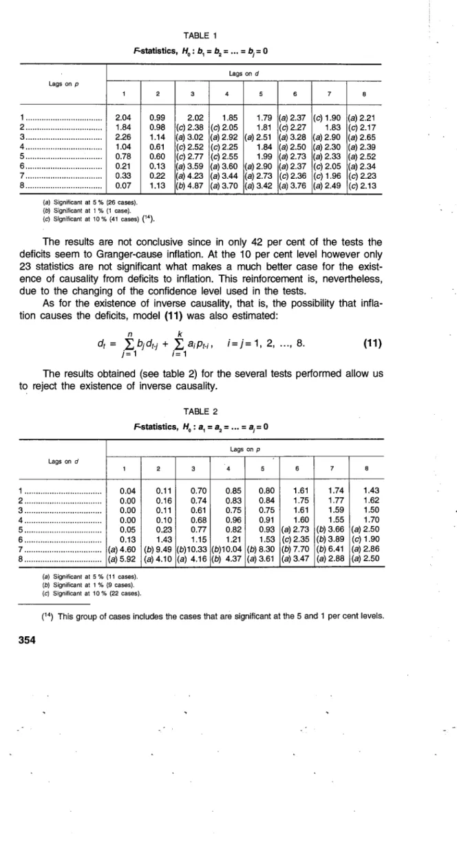
With the number of lags ranging from 1 to 8 for both variables an exhaus-tive set of tests was performed and 64 F-statistics were obtained. From those results, shown in table 1, 26 statistics are significant at the 5 per cent level and 1 at the 1 per cent level that is, in 27 of the 64 situations tested one can-not accept the null hypothesis, H₀ : b₁

= ... =

bj

=

0.

(13) With 0(21) < _t!0_1 we accept the hypothesis that the residuals are a white noise.

TABLE 1

~statistics, H₀ : b₁ = b₂ = ... = b₁ = 0

Lags on p

1

1 ... 2.04 2 ... 1.84 3 ... 2.26 4 ... 1.04 5 ... 0.78 6 ... 0.21 7 ... 0.33 8 ... 0.07 (a) Significant at 5 % (26 cases). (b) Significant at 1 % (1 case).

2 0.99 0.98 1.14 0.61 0.60 0.13 0.22 1.13

(c) Significant at 10% (41 cases) (14_).

Lags on d

3 4 5

2.02 1.85 1.79 (c) 2.38 (c) 2.05 1.81 (a)3.02 (a) 2.92 (a) 2.51 (c) 2.52 (c) 2.25 1.84 (c) 2.77 (c) 2.55 1.99 (a) 3.59 (a) 3.60 (a)2.90 (a)4.23 (a)3.44 (a)2.73 (b) 4.87 (a)3.70 (a) 3.42

6 7 8

(a)2.37 (c) 1.90 (a) 2.21 (c) 2.27 1.83 (c) 2.17 (a)3.28 (a) 2.90 (a) 2.65 (a)2.50 (a)2.30 (a)2.39 (a) 2.73 (a)2.33 (a)2.52 (a) 2.37 (c) 2.05 (a)2.34 (c) 2.36 (c) 1.96 (c) 2.23 (a) 3.76 (a) 2.49 (c) 2.13

The results are not conclusive since in only 42 per cent of the tests the deficits seem to Granger-cause inflation. At the 10 per cent level however only 23 statistics are not significant what makes a much better case for the exist-ence of causality from deficits to inflation. This reinforcement is, nevertheless, due to the changing of the confidence level used in the tests.

As for the existence of inverse causality, that is, the possibility that infla-tion causes the deficits, model (11) was also estimated:

n k

dr = "L,bjdt-j + "L,a;p1_;, i=j=1, 2, ... , 8.

j=1 i=1

(11)

The results obtained (see table 2) for the several tests performed allow us to reject the existence of inverse causality.

Lags on d

1

1 ... 0.04 2 ... 0.00 3 ... 0.00 4 ... 0.00 5 ... 0.05 6 ... 0.13 7 ... (a)4.60 8 ... (a) 5.92 (a) Significant at 5% (11 cases). (b) Significant at 1 % (9 cases). (c) Significant at 10% (22 cases).

2 0.11 0.16 0.11 0.10 0.23 1.43 (b) 9.49 (a) 4.10

TABLE 2

Lags on p

3 4 5

0.70 0.85 0.80 0.74 0.83 0.84 0.61 0.75 0.75 0.68 0.96 0.91 0.77 0.82 0.93 1.15 1.21 1.53 (b)10.33 (b)10.04 (b) 8.30 (a) 4.16 (b) 4.37 (a) 3.61

6 7 8

1.61 1.74 1.43 1.75 1.77 1.62 1.61 1.59 1.50 1.60 1.55 1.70 (a) 2.73 (b)3.66 (a) 2.50 (c) 2.35 (b)3.89 (c) 1.90 (b)7.70 (b) 6.41 (a)2.86 (a)3.47 (a) 2.88 (a) 2.50

From the 64 statistics F, 11 are significant at 5 per cent and 9 are signifi-cant at 1 per cent. Even at 1 0 per cent we can only reject 22 null hypothesis and have to accept it in all the remaining 42 cases.

2.3 - Choice of lags length

A key element for this kind of empirical research is the number of lags allowed for each variable. The bigger the number of lags the bigger is the number of coefficients that have to be estimated which can reduce drastically the de-grees of freedom for each equation. In a multivariate system with

M

variables and

p

lags, the number of parameters to estimate for each equation, including a constant, could be Mp + 1. It is important then to obtain the optimal lags for each variable following for instance the example of McMillin (1986), Ahking and Miller (1986) or Barnhart and Darrat (1988).

One of the criteria

(1

5_{) normally used to obtain the optimal lag length of a .}

variable in a regression is the AIC (Akaike Information Criterion). After imposing the maximum number of lags at eight, the AIC criteria was used in order to obtain the lag length for the two variables included in (11). The resulting model includes four lags for inflation and eight lags for the deficits,

Pt = -0.80 Pt-1 + 0.03 Pt-2 + 0.24 Pt-3-0.30 Pt4 (12) (- 0.46) (0.16) (1.32) (- 1. 79)

+

0.09 d1•1 - 0,41 d1.2 ~ 0.30 d1. 3 -0.03 d14 (0.27) (- 1.61) (- 2.04) (- 0.20) - 0.24 d1

-s-

0,06 dr-6-0.14 d1.7 + 0.02 d1.a

(- 1.61) (- 0.38) (- 0.98) (0.16)

R2

=

0.30 Q (18)

=

11.50 F (8,32)

=

2.39.

The value of the F-statistic for model (12) is significant at the 5 per cent level which allows one to accept the existence of causality from deficits to inflation.

2.4 - A trivariate model

In order to improve the results a monetary variable, the money stock measured by M2., was added to the original bivariate process. It would be pos-sible then to study not only the direct causality from deficits to inflation but also the indirect effect through the money stock.

The observations for M2 are the end of quarter values as published in the Bank of Portugal Quarterly Bulletins. After taking the logarithms, the Box-Jenkins methodology was used and the series filtered by an ARIMA (1, 2, 0) (1, 0, 1)4 ,

which includes autoregressive and moving average seasonal parameters. The

estimati<~>n of the process, which may be written as:

and where M is the logarithm of M2, produced the following results:

Mt

= -

0.627 Mt-1 + 0.8038 Mt-4-0.4132 et-4 + et (14)

(- 5.12) (9.49) (- 2.24)

FP

=

0.999

o

(21)

=

4.65.

The adjusted model is stationary since we have I ¢1 I < 1 and I <1>4 I < 1

being also invertible because the moving average coefficient satisfies the condi-tion I 84 I < 1 . The Q-statistic allows one to accept that the series of the residuals

is probably a white noise.

Using the residuals from model (14) we can estimate a trivariate model and assess the additional contribution of M2 to inflation. The proposed model is:

k n m

Pt

=

L

ai Pt-i +

L

bj dt-j

=

L

Csmt-s

i=1 j=1 5=1

(15)

where we limit the maximum number of lags to four in order to avoid loosing too many degrees of freedom (k =

n

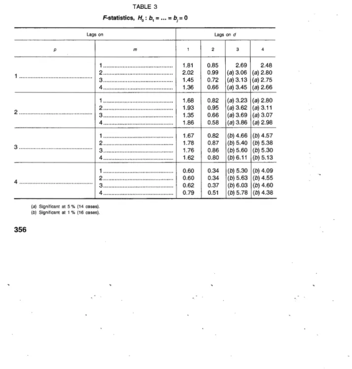
= m = 4).

TABLE 3

F-statistics, H0 : b1 = ...

=

bi

=

0

Lags on

p m

1 ... . 1 ··· 2 ... . 3 ... . 4 ... . 1 ... . 2 ... . 2 ··· 3 ... . 4 ... . 1 ··· 2 ... . 3 ... 3 ... .

4 ... . 1 ··· 4 ··· 2 ... . 3 ... . 4 ... .

(a) Significant at 5% (14 cases). (b) Significant at 1 % (16 cases).

1.81 2.02 1.45 1.36 1.68 1.93 1.35 1.86 1.67 1.78 1.76 1.62 0.60 0.60 0.62 0.79

Lags on d

2 3 4

The values for the F-statistics, computed to evaluate the existence of cau-sality from deficits to inflation are given in table 3. For the 64 (43 _{= 64)} F-statis-tics obtained, 14 are significant at the 5 per cent level and 16 are significant at the 1 per cent level that is, we can accept the existence of causality from defi-cits to inflation in 47 per cent of the tests made

(1

6). The presence of the money stock as an explanatory variable in the inflation regression improves slightly the evidence of causality between deficits and inflation.

The choice of the adequate lags for each variable was also made using the AIC and the result was a specification with four, three and one lags respec-tively for inflation, deficits and money:

Pt=-0.05 Pt-1 + 0.29 Pt-2 + 0.32 Pt-3-0.29 Pt-4 (16)

(- 0.03) (2.27) (2.47) (- 2.22)

+ 0.35 dt-1 - 0,02 d1•2 - 0.45 d1.3 - 1.30 m1.1

(2.05) (- 0.18) (- 3.87) (- 1.1 0)

R2

= 0.32 Q (18) = 1 0.94 F (3,37) = 5.30.

The adjustment presented in (16) is similar to the one produced earlier by the bivariate process, model (12). One can see that the coefficients of the first three lags of the deficits have the same sign, being the first one now statisti-cally different from zero, and that the lags in inflation are also similar. Further-more, the F-statistic now allows the acceptance of the hypothesis of causality at the 1 per cent level while in model (12) that hypothesis was accepted only at the 5 per cent level.

Concerning the issue of inverse causality the causality tests performed led to the rejection of the null hypothesis in 4 cases at the 5 per cent level and in 5 cases at the 1 0 per cent level. It is possible then to reject the existence of inverse causality.

The causality from deficits to money was also evaluated. At the 10 per cent level none of the F-statistics computed is significant. There is therefore no evidence of the inflationary effects of the deficits through money supply as stated in the monetarist paradigm. This result, in parallel with the evidence of the ex-istence of direct causality from deficits to inflation, seems to indicate that the deficits produce a rise in the price level mainly through aggregate demand.

Maybe the absence of causality from deficits to the money stock might be explained by a bad choice of the monetary aggregate. Hamburger and Zwick (1981) say that the acquisition of public debt by the Central Bank is probably going to influence more the monetary base than any other wider monetary ag-gregate. Following those lines we replaced the M2 aggregate by the monetary base in our trivariate process.

The univariate adjustment obtained for the monetary base was an ARIMA (0, 1, 0) (1, 0, 1 )4 written with the lag operator as:

(17)

and where MB is the logarithm of the monetary base. The estimation results were:

MB1 = 0.9584 MB14 - 0.8565 t:14 + t:1 (18)

(19.08) (- 7.98)

~ = 0.982 Q (21) = 1 0.59.

The adjustment reported in (18) is stationary and invertible and one can not reject the hypothesis that the residuals are purely random. Using the series of the residuals from (18) the trivariate model was once again estimated now with the monetary base replacing the aggregate M2.

The monetization hypothesis is once again rejected since from the 64 F-statistics calculated not even one is significant at the 1 0 per cent level. As for the inverse causality hypothesis the tests led us to reject the null hypothesis in 3 cases at the 5 per cent level and in 9 cases at the 1 0 per cent level. The absence of causality from inflation to the deficits in a trivariate model is there-tore accepted either with the money stock or with the monetary base.

When the monetary base is included as a regressor in the model tor infla-tion:

4 4 4

Pt = "Lai Pt·i +

L

bj dt·j +

'L

Csmbr.s, (19)

i=1 j=1 S=1

we have a little more evidence of the existence of the deficits-inflation causality. In tact, 32 of the F-statistics calculated

(1

7) are significant at the 10 per cent level, or, put in another way, in halt of the tests made there is evidence that the deficits Granger-cause inflation.

For the process given in (19) the AIC criterion is minimized with tour lags tor inflation, three lags tor the deficits and also three lags tor the monetary base, the result being presented below:

Pt = 0.08 Pr-1 + 0.22 Pr-2 + 0.30 Pt-3-0.31 Pt-4 (20) (0.64) (1.77) (2.45) ( - 2.42)

+ 0.28 dt·1-0,02 dt·2-0.41 dt·3

(1.69) (0.19) (- 3.69)

+ 0.1 0 mb1•1- 0,23 mb1.2+ 0.29 mb1.3

(0.65) (- 1.54) (1.90)

F/2

= 0.37 Q (18) = 12.73 F (3,35) = 4.61.

The coefficients for the lagged regressors of the deficit in (20) are quite similar to the ones estimated when the monetary aggregate M2 was used [see regression (16)]. In both models the first lag of the deficits affects positively the price level while the third lag has a negative contribution.

3 - Concluding remarks

The empirical findings reported above allow us to conclude that, in the Portuguese case, there is some evidence of causality from the deficits to infla-tion, the deficit being a proxy build with the stock of internal direct debt. This is true in a bivariate model and also in a trivariate model which includes the mone-tary base or even the money stock measured by M2. The contribution of the deficits to inflation is positive and the coefficient of the first lag of the deficits is also statistically significant, either with the monetary base or with the monetary aggregate M2.

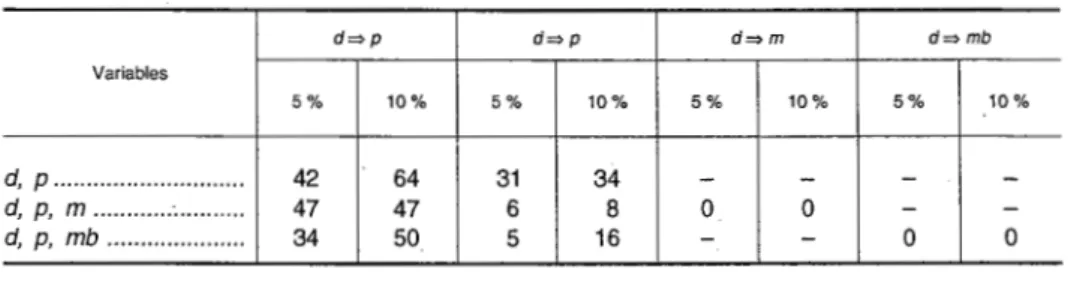
Table 4 presents a summary of the percentage of F-statistics significant at the 5 and 1 0 per cent level. There is no evidence that inflation causes the deficits and the same is true for the monetization hypothesis, so that one can assume that the relation between deficits and inflation is probably through aggregate demand.

TABLE 4

Percentage of significant F-statistics (a)

d=> p d=> p d=> m d=> mb

Variables

5% 10% 5% 10% 5% 10% 5% 10%

d, p ... 42 64 31 34

d, p, m ... : ... 47 47 6 8 0 0

d, p, mb _··· 34 50 5 16 0 0

(a) Number of signijicant cases in the 64 tests made for each causality hypothesis.

The empirical evidence presented above must be used carefully since we only used a maximum of three variables at the same time. This approach is justified, as it was already said, by the number of coefficients that have to be estimated and by the sample size. Therefore it would be advisable to estimate a multivariate model including also the interest rate of the public debt and some measure of the exchange rate. The stock of external public debt could also be added to the stock of internal public debt. Maybe some of the expectations that one usually has about the monetization of the deficit could then be validated.

Concerning the issue of the relation between deficits and inflation there is little known work for Portugal. There are however some calculations made by Santos (1992) who estimates a reduced form equation for inflation where the general government deficit is included as an explanatory variable. The results

(1

8₎ led him also to conclude that the deficit appears to be inflationary.

Another set of results for Portugal is provided by Costa (1984) who also used annual c;fata for the period 1960-1980. The estimation of reaction functions

allowed him to conclude that although deficits appear to have been monetized during the period 1960-1973, it is not possible to obtain empirical evidence of that relation in the period 197 4-1980.

REFERENCES

AFONSO, Antonio M. P. (1992), «Defices publicos e inflac;ao••, October, MSc dissertation, Universidade Tecnica de Lisboa, ISEG, Lisboa.

AHKING, Francis A., and MILLER, Stephen M. (1985), «The Relationship Between Government Deficits, Money Growth, and Inflation», Journal of Macroeconomics, vol. 7, n.Q 4, Autumn, pp. 447-467.

BARNHART, Scott W., and DARRAT, Ali F. (1988), «Budget Deficits, Money Growth and Causal-ity: Further OECD Evidence», Journal of International Money and Finance, vol. 7, n.Q 2, June, pp. 137-149.

SARRO, Robert J. (1989), «The Ricardian Approach to Budget Deficits», The Journal of Economic

Perspectives, vol. 3, n.Q 2, pp. 37-54.

BERNHEIM, B. D. (1989), «A Neoclassical Perspective on Budget Deficits .. , The Journal of

Eco-nomic Perspectives, vol. 3, n.Q 2, pp. 55-72.

BLINDER, Alan S. (1983), «On the Monetization of Deficits» in Meyer, Laurence (ed.), The

Eco-nomic Consequences of Government Deficits, Kluwer-Nijhoff Publishing, Boston.

COSTA, Jose (1984), «Government budget deficits, money supply, and inflation in Portugal»,

Economia, vol. vm, n.Q 1, January, pp. 97-116.

DWYER,G. P., Jr. (1982), «Inflation and Government Deficits», Economic Inquiry, vol. xx, n.Q 3, July, pp. 315-329.

- - (1984), «Inflation and Government Deficits: a Reply .. , Economic Inquiry, vol. xx11, n.Q 4, Oc-tober, pp. 597-601.

EISNER, Robert (1989), «Budget Deficits: Rhetoric and Reality», The Journal of Economic

Per-spectives, vol. 3, n.Q 2, pp. 73-93.

GRAMLICH, E. M. (1989), «Budget Deficits and National Savings: are Politicians Exogenous», The

Journal of Economic Perspectives, vol. 3, n.Q 2, pp. 23-35.

GRANGER, C. W. (1969), «Investigating Causal Relations by Econometric Models and Cross-Spectral Methods», Econometrica, vol. 37, pp. 424-438.

HAFER, R. W., and HEIN, S. E. (1988), «Further Evidence on the Relationship Between Federal Government Debt and Inflation», Economic Inquiry, vol. xxv1, n.Q 2, April, pp. 239-251. HAMBURGER, Michael J., and ZWICK, Burton (1981), «Deficits, Money and Inflation», Journal of

Monetary Economics, vol. 7, n.Q 1, January, pp. 141-150.

HSIAO, C. (1981), «Autoregressive Modelling and Money-Income Causality Detection» Journal of

Monetary Economics, 7, pp. 85-106.

KING, Robert G., and PLOSSER, Charles I. (1985), «Money, Deficits and Inflation», in Brunner, Karl, Meltzer, and Allan H. (eds.) Understanding Monetary Regimes, Carnegie-Rochester Conference Series on Public Policy, 22, pp. 147-196.

LJUNG, G. M. and BOX, G. E. P. (1978), «On a measure of lack of fit in time series models»,

Biometrika, 65, 2, pp. 297-303.

MCMILLIN, W. Douglas (1986), «Federal Deficits, Macrostabilization, Goals, and Federal Reserve Behavior;., Economic Inquiry, vol. xx1v, n.Q 2, April, pp. 257-269.

MILLER, Preston J. (1983a), «Examining the Proposition that Federal Budget Deficits Matter», in Meyer, Laurence (ed.), The Economic Consequences of Government Deficits, Kluwer-Nijhoff Publishing, Boston.

- - (1983b), «Higher Deficit Policies Lead to Higher Inflation», Federal Reserve Bank of

Minneapolis Quarterly Review, Winter, pp. 8-19.

OLIVEIRA, Filomena R. and GARCIA, Antonio (1989), «Moeda e inflac;ao em Portugal- A exis-tencia de causalidade», Gabinete de Estudos do Banco de Portugal, Documento de Trabalho n.Q 16.

PANKRATZ, A. (1983), Forecasting With Univariate Box-Jenkins Models: Concepts and Cases,

Wiley.

PIERCE, David A., and HAUGH, Larry D. (1977), «Causality in Temporal Systems», Journal of

Econometrics, vol. 5, n.Q 3, May, pp. 265-293.

SANTOS, Joao Nunes dos (1989), «Causalidade entre moeda e rendimento da economia portuguesa: 1958-1984», Economia, vol. XIII, n.Q 3, October, pp. 335-357.

- - (1992), «Budget Deficits and Inflation: Portugal and the other EC High Debt Countries»,

Estudos de Economia, vol. xu, n.Q 3, April - June, pp. 245-253.

SCHWERT, G. William (1979), «Tests of Causality: the Message in the Innovations••, in Brunner, K., and Meltzer, A. H. (eds.), Three Aspects of Policy and Policymaking: Knowledge, Data and Institutions, Carnegie-Rochester Conference Series ou Public Policy, 10.

THORNTON, DanielL., and BATTEN, Dallas S. (1985), «Lag-Length Selection and Tests of Granger Causality between Money and Income», Journal of Money, Credit and Banking, May, pp. 164-178.