Eurasian Journal of Business and Economics 2011, 4 (8), 1-12.
Reconsidering the Relationship between Oil
Prices and Industrial Production: Testing for
Cointegration in some of the OECD Countries
Ibrahim Halil EKSI
*, Berna Balci IZGI
**,
Mehmet SENTURK
***Abstract
This paper investigates the effects of crude oil prices on the industrial production for some of the OECD countries. According to it, the empirical results sign that there is statistical meaningful short term causality from crude oil price to industrial production in all countries except France. In France however, causality is from industrial production to oil price in short run. The error correction mechanism is run for US. The causality is from oil price to industrial production in long run for US. These results show us that oil prices do affect industrial production index. Another interesting finding that, similar results were observed for oil exporting and importing countries such as Saudi Arabia and Iran as well. This situation is important that firm sensitivity towards oil price shows a similarity among the countries.
Keywords: Crude Oil Price, Industrial Production, Cointegration, VAR.
JEL Code Classification: D01, L60, F14.
*
University of Kilis 7 Aralik, Turkey E-mail: [email protected]
1. Introduction
Crude oil is the world's most actively traded commodity both in volume and in value. Until the creation of futures markets in mid 1980s, crude oil was largely sold by producers to consumers under long term contracts. Since then the oil market has become liberal and highly liquid in which price discovery has been concentrated around three marker crudes - WTI, Brent and Dubai. These markers are considered to be the reference for all oil traded worldwide (Cuaresma, Jumah, Karbuz, 2007:114). In the literature OECD countries for which are studied widely -the United States, -the United Kingdom, Canada, France, Germany, -the Ne-therlands, Italy, and Japan--differ in ways which could be expected to influence their vulnerability to oil price shocks (Jones and Leiby, 1996:21). They differ in their industrial structures, their compositions of overall energy supply, their societies’ and governments priorities and macroeconomic and microeconomic policies, and their labor market structures and institutions. Also, not all the data from these countries are exactly comparable, as Mork et al. (1994, pp. 25-26) note in some detail. Darby (1982, p. 741) has questioned the quality of the relevant data from France, Italy, and Japan, while Mork et al. (1994, p. 27) have raised similar questions about German GDP data as a result of their statistical performance. Accordingly one would not expect to find exactly the same response pattern to any shock across these countries.
It is widely accepted that fluctuations in price of oil have substantial real effects on macroeconomic variables (Hamilton, 1983:228-248; Loungani 1986:536-539; Peron 1989:1361-1401). Oil prices may have an impact on economic activity through various channels (Lardic and Mignon, 2008:847-855).
According to Hamilton, oil price increases seem to be one of the main cause of recessions in USA prior to 1972 (Hamilton, 1983:228-248). Within a vector autoregression (VAR) framework Hamilton (1983, 1996) have found a strong causal and negative correlation between oil price change and real U.S. GNP growth from 1948 to 1980. When the sample period is extended to 1988:2 the correlation becomes only marginally significant and that there are asymmetric effects. GNP growth has a definite negative correlation with oil price increases and an insignificant correlation with oil price decreases. Many of the quarterly oil price increases observed since 1985 are corrections to even bigger oil price decreases from the previous quarter. When one looks at the net increase in oil prices over the year, recent data are consistent with the historical correlation between oil shocks and recessions (Hamilton, 1996:215-220).
their original estimation period (1960:I-1993:IV). Besides this the increased volatility of oil prices in their period (1960:I-1993:IV) was found (Darrat, Gilley and Meyer, 1996:158). However, Hamilton obtained his "evidence" of a significant relationship with the real economy in his paper, that their estimation period is characterized by several major episodes of oil price changes, ranging from the hikes of the mid-1970s, to the sharp declines of the early 1980s, to the more recent spikes of the Gulf War era.
In the mid 1970s, downturns in the industrial production would probably occur at any event and the oil price increase served to deepen a recession that was already on the way (Burbidge and Harrison, 1984:459-484). Burbidge and Harrison (1984), found significant impacts of oil and energy shocks on real activity for the U.S. using annual data. They have used an unrestricted systems of equations estimated for five countries in OECD for the period 1962 to 1982 and estimated a seven-variable vector autoregression (VAR) for each. The main finding of their study was a significant difference between the effects of the 1973-1974 set of oil price shocks and those of the 1979-1980 shocks .
Mork (1989), was the first who attained the asymmetry of the oil price shocks on economic activities. He separated the real oil price variable into upward and downward movements in order to analyze the oil price increases and decreases. In Mork’s paper, the results were weaker than Hamilton’s results (Mork, 1989:740-744). However in both of the studies any oil price change regardless of direction causes some costly resource allocation. Those two effects worked against and could largely offset each other when oil prices fell while they operated in the same direction when oil prices increased. Mork and Olson (1994) again verified that there was a negative and significant relationship between an oil price increase and national output, while no statistical significance could be attributed to them when the oil price falls (Mork and Olson, 1994:19-35).
employment to oil price shocks is asymmetric, the response to postive shocks is ten times larger than that to negative shocks (Davis and Haltiwanger, 2001:465-512).
Blanchard and Gali (2007), have used structural VAR technique to analyze the effects of oil price changes on macroeconomic variables. Their results show that, the estimated response for employment and output become weaker over time, with point estimates becoming slightly positive for the most recent period. There were other adverse shocks in 1970s; the price of oil explains only part of the stagflation episodes of the 1970s (Blanchard and Gali, 2007: 1-78).
The effects of a given change in the price of oil have changed substantially over time. They explain that one of the reasons for this change is the decline in wage rigidities. According to Alper and Torul (2008), oil price increases do not significantly affect the manufacturing sector in aggregate terms, some sub-sectors are adversely affected. They have taken into account exogeneity of oil prices, extreme oil reliance and import-dependence, as well as asymmetric responses of oil product prices to world crude oil price changes (Alper and Torul, 2008). According to Blanchard and Gali (2007), it appears that there are three potential changes in economies over time. These are behavior of wages, role of monetary policy and importance of oil. The role of monetary policy has changed since 1970s. In 1970s the central banks didn’t know how to react and central banks credibility was low. In the 2000s supply shocks are no longer new, monetary policy is clearly set and credibility is much higher. Thirdly the importance of oil in the economy has declined over time. Increases in the price of oil have led to substitution away from oil, and a decrease in the relevant shares of oil in consumption and in production (Blanchard and Gali, 2007:1-78).
output of the main manufacturing industries in six OECD countries. The pattern of responses to an oil price shock by industrial output is diverse across the four European Monetary Union (EMU) countries under consideration (France, Germany, Italy, and Spain), but broadly similar in the UK and the US (Rodriguez, 2008:3095-3108).
Herrera,Lagalo and Wada (2010) have found that costly reallocation of factor inputs across sectors might play an important role in explaining the response of industrial production to oil price shocks, even though the response of real GDP has been shown not to be significantly asymmetric. According to Mehrara and Sarem (2009), there is a strong causality from oil price shocks to output growth for Iran and Saudi Arabia. Moreover, the oil prices–output relationship in these two countries appears more significant when asymmetric specifications are used to model the relationship between variables. In the case of Indonesia, however, none of the oil proxies have any significant effect on output both in the short and long run. The results confirm the relatively successful experience of countries such as Indonesia in the diversification of the real sector to minimize the harmful effects of oil booms and busts. Reyes and Quiros (2005) have found that raises in oil price affects in a negative and statistically significant way to stock returns and to industrial production, but the effect on stock returns is stronger than on industrial production.
2. Methodology and Data
2.1. Methodology
There is a huge literature about the effects of oil prices on macroeconomic variables. However, this study has a different aspect from the others in the sense that, it specifically deals with the effects on industrial production in a causality relationship. The relationship between variables investigated with Johansen Cointegration Approach. For cointegration testing, Johansen test is generally used (Trešl and Blatná, 2007:299).
Granger and Engle (1987) in their studies have indicated that linear combinations of two or more unstationary series may be stationary. If there is a stationary linear combination exists in this kind of unstationary series, these series are called as cointegrated. This linear stationary combination shows the longrun relationship among the variables and is called as cointegrated equation. We used cointegration tests, based on the methodology of Johansen’s VAR model (Engle and Granger,1987:270). Pth VAR model is shown below:
t t p
t p t
t A y A y Bx
y = 1 −1 + ... + − + + ε
(1)
1
1 1
p
t t i i t i t t
y y− =− y− B x ε
∆ = Π +
∑
Γ ∆ + + (2)In this equation, ıt is defined as
∏ = ∑ = −
p
i 1 A i I and Γ = −∑ = +
p i
j j
i 1 A (3)
The coefficient of П shows that if the reduced rank (r)is smaller than the endogeneous variable number (r<k if), than П=αβ’ and β’y is I(0)and there exist kxr number of α and β matrices. r shows the number of cointegration relationship and each column of β is the cointegration vector. Two test statistics are used for testing the cointegration relationship in number r. The first one of these is called as trace test. In this test H0 investigates r and H1 investigates k number of cointegration relationship (k is the number of endogeneous variables). Trace statistics is calculated as shown below (Johansen and Juselius, 1990:170)
∑
= + −−
= k
r
i i
tr r k T
LR ( / ) 1 log( 1 λ ) (4)
λi is the ith eigen value of П matrice. The second test statistics is called as eigen value statistics. It investigates r+1 number of cointegration relationship against r. Eigen value statistics is calculated as shown below.
) 1
log( )
1 /
( 1
max r r + = −T − r+
LR
λ
(5)2.2. Data
The study’s data were monthly and covered from 1997:1 to 2008:12. Industrial production data were taken from OECD web site and Energy Information Administration (EIA) for the oil prices. The reason why these country groups have been used is that, some of the OECD countries have changed their index measuring in some years (Italy 1995-05, Belgium 1996-06). Such countries were not included in the analysis, instead Turkey, US, Germany, Spain, France, South Korea and Japan were included. US in one side, while Turkey, Germany, Spain and France in the other side and South Korea and Japan represent far east countries in the analysis.
The following notations were used for the above model:
LOP: Logaritmic values of oil prices(world),
LIP: Logaritmic values of index of industrial production, ∆LOP: First log difference of oil price,
∆LIP: First log difference of industrial production
3. Results
3.1. Unit Root and Cointegration Tests Results
A cointegrating relationship exists between non-stationary series, if there is a stationary linear combination between them. Therefore, one needs to test the stationarity of the series first. Augmented-Dickey-Fuller (ADF) and Phillips-Perron (PP) tests and KPSS tests are used to determine whether or not the series are stationary.
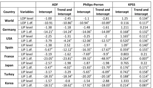
In the Table 1 superscript a denotes significance at 1% critical level. Optimum lag lengths are set according to SC for ADF, Newey-West method for PP and KPSS.
The ADF and PP tests have the null hypothesis of existence of a unit root, rejection of which indicates stationarity. Table 1 presents the results for the unit root tests.
Table 1: Unit Root Test Results
ADF Philips-Perron KPSS
Country Variables Intercept Trend and
Intercept Intercept
Trend and
Intercept Intercept
Trend and Intercept
World LOP level -1.00 -2.45 -1.1 -2,81 1.25 0.134
a
LOP 1.df. -10.91 -10.86a -10.94a -10.89a 0.116 0.117a Germany LIP level -1.38 -1.18 -1.48 -1.61 1.211 0.214 LIP 1.df. -14.21a -14.24a -14.06a -14.09a 0.168a 0.132a USA LIP level -2.25 -1.31 -3.25 -2 1.165
a 0.111a
LIP 1.df. -3.79 -4.24a -12.06a -12.57a 0.520a 0.136a Spain LIP level -1.38 2.52 -1.97 0 1.09
a
0.140a LIP 1.df. -5.67a -12.12a -16.35a -17.67a 0.359a 0.155a
France LIP level -3.19 -1.62 -7.69
a
-9.9a 0.803 0.21 LIP 1.df. -23.05a -23.81a -39.32a -48.97a 0.264a 0.007a
Japan LIP level -2.57 -1.98 -1.87 -1.98 0.765 0.22 LIP 1.df. -3.47a -4.02a -15.83a -15.79a 0.176a 0.171a Turkey LIP level -3.17 -3.29 -5.65
a
-6.09a 0.742a 0.158a LIP 1.df. -18.35a -18.34a -20.20a -20.18a 0.188a 0.114a Korea LIP level -1.57 -0.8 -1.54 -2.88 1.333 0.124
a
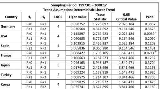
Table 2: Cointegration Test Results
Sampling Period: 1997:01 – 2008:12 Trend Assumption: Deterministic Linear Trend
Country H0 H1 LAGS Eigen value
Trace Statistic
0.05
Critical Value Prob.
Germany R=0 R=1 4 0.058752 1.273.097 2.026.184 0.3857 R≤1 R=2 0.030564 4.314.692 9.164.546 0.3673
USA R=0 R=1 4 0.145897 2.769.423 2.026.184 0.0039
a
R≤1 R=2 0.040685 5.773.437 9.164.546 0.2090
Spain R=0 R=1 4 0.102915 2.456.237 2.526.184 0.1203 R≤1 R=2 0.065836 9.066.280 9.164.546 0.1431
France R=0 R=1 5 0.088427 1.793.105 1.549.471 0.0211
b
R≤1 R=2 0.106663 3.154.523 3.841.466 0.1232
Japan R=0 R=1 5 0.046163 8.946.187 1.549.471 0.3704 R≤1 R=2 0.017412 2.423.996 3.841.466 0.1195
Turkey R=0 R=1 2 0.069224 1.132.919 1.549.471 0.1920 R≤1 R=2 0.008575 1.214.307 3.841.466 0.2705
Korea R=0 R=1 4 0.059825 1.219.972 1.549.471 0.1476 R≤1 R=2 0.025741 3.624.895 3.841.466 0.1169 Superscripts a and b denote rejection of the null hypothesis at the 1% and 5% levels of significance, respectively.
3.2. Granger Causality and Vector Error Correction Models
According to this approach, if two variables are cointegrated, then, there is an error correction mechanism (ECM) to revise instability in short term (Engle and Granger, 1987). ECM is used to see the speed of adjustments of the variables to deviations from their common stochastic trend. ECM corrects the deviations from the long-run equilibrium by short-long-run adjustments. This shows us that changes in independent variables are a function of changes in explanatory variables and the lagged error term in cointegrated regression. Granger and Engle (Granger and Engle, 1987) have showed that in case of a cointegration between the variables, there may be one way or two way Granger-causality between the variables which have stochastic error terms in I (0). Thus, regression is purified from spurious regression. Error terms are derived for France and US. ECM’s of France and US are shown in Tables 3 and 4.
Table 3: ECM for France
F
ra
n
ce
Dependent Variable: ∆LOP Causality Results Variables Prob. Coefficient Short Term Long Term
ECT t-1 0.0162 0.979072
∆LIP → ∆LOP No
∆LOP t-1 0.6286 0.042674
∆LOP t-2 0.3882 -0.076956
∆LOP t-3 0.0976 0.153894
∆LOP t-4 0.3602 -0.086248
∆LIP t-1 0.0144 -0.913332
∆LIP t-2 0.4710 -0.412290
∆LIP t-3 0.1823 -0.785160
∆LIP t-4 0.3196 -0.523671
∆LIP t-5 0.4011 -0.306540
Constant 0.8307 0.001763 f-wald test 0.0903 19515 c
Dependent Variable: ∆LIP Causality Results Variables Prob. Coefficient Short Term Long Term
ECT t-1 0.0000 0.474431
No No
∆LIP t-1 0.0000 -0.844381
∆LOP t-1 0.2756 -0.029167
∆LOP t-2 0.1121 -0.044069
∆LOP t-3 0.2453 -0.032323
∆LOP t-4 0.6401 0.013060
Constant 0.7763 -0.000715 f-wald test 0.3078 1214499
Table 4: ECM for US
1U
S
A
Dependent Variable: ∆LOP Causality Results
Variables Prob. Coefficient Short Term Long Term ECT t-1 0.0003 0.997188
∆LIP → ∆LOP No ∆LOP t-1 0.6797 0.033770
∆LIP t-1 0.0424 2232072
Constant 0.9111 0.000871 f-wald test 0.0424 4198239 b
Dependent Variable: ∆LIP Causality Results
Variables Prob. Coefficient Short Term Long Term ECT t-1 0.0701 -0.039827
b
∆LOP → ∆LIP ∆LOP → ∆LIP ∆LIP t-1 0.8750 -0.013601
∆LOP t-1 0.0016 0.020229
∆LOP t-2 0.0865 0.011284
Constant 0.1058 0.000976 f-wald test 0.0017 6687886 b
1
In ECM for US, there seems to be no long term relationship from industrial production index to crude oil prices so the ECM didn’t work. For the f-wald test for short term, there was causality from industrial production to oil prices. Both long and short term causality was found from crude oil prices to industrial production index and ECM has worked for US. Results of the Granger causality test are shown below:
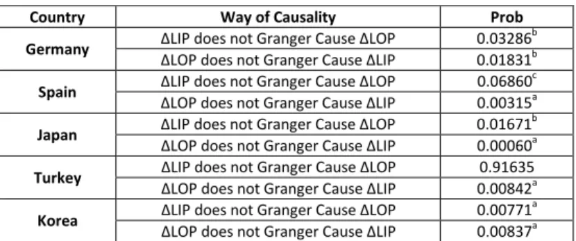
Table 5: Granger Causality Test for Selected OECD Country
2 Country Way of Causality ProbGermany ∆LIP does not Granger Cause ∆LOP 0.03286
b
∆LOP does not Granger Cause ∆LIP 0.01831b Spain ∆LIP does not Granger Cause ∆LOP 0.06860
c
∆LOP does not Granger Cause ∆LIP 0.00315a Japan ∆LIP does not Granger Cause ∆LOP 0.01671
b
∆LOP does not Granger Cause ∆LIP 0.00060a
Turkey ∆LIP does not Granger Cause ∆LOP 0.91635 ∆LOP does not Granger Cause ∆LIP 0.00842a Korea ∆LIP does not Granger Cause ∆LOP 0.00771
a
∆LOP does not Granger Cause ∆LIP 0.00837a
In Granger causality test, there is a casual relationship from crude oil prices to industrial production index. A causal relation from industrial production to oil prices is valid except for Turkey.
4. Conclusion and Policy Implications
This study tried to understand the causality between industrial production indexes and crude oil prices for 7 OECD countries. Empirical findings show that, there is statistical meaningful short term causality from crude oil price to industrial production in all countries except France. In France however, causality is from industrial production to oil price in short run. The error correction mechanism is run for US. The causality is from oil price to industrial production in long run for US. These results show us oil prices do affect industrial production index. The conspicuous point here is that the relationship between these two variables makes no difference for the oil balance among these countries. In other words, similar results were observed for oil exporting and importing countries.
The causality from industrial production to oil price can be associated with oil demand. Foreseeing the oil price has crucial importance for these countries. An obvious potential direction for future research may be that the expansion of the present analysis to a multivariable (CPI, real exchange rate, energy price index may be included) context. With this way it is possible to explain the dimension and
2
existence of the relationship between the oil price and industrial production more accurately. Industrial production is very crucial for economies and especially for the manufacturing firms. The crude oil price may be the sign of ambiguity as well as a cost element. The firms are unconstrained by the volatility of oil prices. The firms could be successful as far as they can reflect those price changes to their costs. One of the most important indicators of firm behavior towards oil prices is industrial production itself.
We thus propose policy suggestions to solve the oil price effect on industrial production for these countries: foreseeing the crude oil price is still very crucial for these economies. In spite of the knowledge we have about the new energy alternatives and the decrease in usage of oil products, oil still has a vital importance on production itself. Therefore, enhancing oil supply security and guaranteeing oil supply to set up national strategic oil reserve for oil dependent industries is very crucial.
References
Alper, E. and Torul, O. (2008), “Asymmetric Effects of Oil Prices on the Manufacturing Sector in Turkey”, 31st IAEE International Conference in Istanbul, June 2008.
Blanchard, O. and Gali, J. (2007) “The Macroeconomic Effects of Oil Shocks: Why Are The 2000s So Different From 1970s”, NBER Working Paper, Vol. 66, pp. 1-78.
Bohi (1989), Energy Price Shocks and Macroeconomic Performance, Resources for the Future, Washington, DC.
Burbidge, J., Harrison, A. (1984), “Testing for The Effects of Oil Price Rises Using Vector Autoregressions”, International Economic Review, Vol. 25, pp. 459-484.
Cuaresma, Jumah,A.,Karbuz,S. (2007), “Modeling and Forecasting Oil Prices: The Role of Asymmetric Cycles”, Working Papers in Economics and Statistics Modeling - University of Innsbruck, Vol. 22, pp. 1-14.
Darby, M. R. (1982), "The Price of Oil and World Inflation and Recession," American Economic Review 72:738-751.
Darrat Ali,F., Gilley Otis,W., Meyer Don,J. (1996), “U.S. Oil Consumption, Oil Prices, and the Macroeconomy”, Empirical Economics.
Davis, S. J., Haltiwanger, J. (2001), “Sectoral Job Creation and Destruction Responses to Oil Price Changes”, Journal of Monetary Economics, Vol. 48, No. 3, pp. 465-512.
Granger, C.W.J., Engle, R. F. (1987), “Co-Integration and Error Correction: Representation, Estimation, and Testing”, Econometrica, Vol. 2, pp. 51-76.
Hamilton, J. (1983), “Oil and The Macroeconomy Since World War II”, Journal of Political Economy, Vol. 2, pp. 228-248.
Hamilton, J. (1996), “This is What Happened to Oil Price Relationship”, Journal of Monetary Economics, Vol. 2, pp. 215-220.
Herrera,A.M; Lagalo, L.G;Wada,T. (2010), “Oil Price Shocks and Industrial Production: Is the Relationship Linear?”, http://people.bu.edu/perron/seminar-papers/HLW_wada.pdf Johansen S., Juselius, K. (1990), “Some Structural Hypotheses in a Multivariate Cointegration Analysis of the Purchasing Power Parity and the Uncovered Interest Parity for UK” Discussion Papers 90-05, University of Copenhagen, Department of Economics.
Jones,D.W; Leiby,P.N. (1996). “The Macroeconomic Impacts of Oil Price Shocks: A Review of Literature and Issues”, Prepared by the OAK Ridge Natıonal Laboratory OAK Ridge, Tennessee 37831 Managed by Martin Marietta Energy Systems, Inc. for the U.S. Department
of Energy under Contract No. DE-AC05-840R21400,
http://www.esd.ornl.gov/eess/energy_analysis/files/Prshock1.pdf
Kilian and Park (2007), Kilian, L., Park, C., 2007. “The Impact of Oil Price Shocks on the U.S. Stock Market” CEPR Discussion Paper No. 6166.
Lardic, S., Mignon, V. (2008), “Oil Prices and Economic Activity: An Asymmetric Cointegration Approach”, Energy Economics, Vol. 30, No. 3, pp. 847-855.
Lee K., Ni S. (2002), “On the Ddynamic Effects of Oil Price Shocks: A Study Using Industry Level Data”, Journal of Monetary Economics Vol. 49, pp. 823–852.
Loungani, P. (1986), “Oil Price Shocks and The Dispersion Hypothesis”, The Review of Economics and Statistics, Vol. 3, pp. 536-539.
Mehrara,M; Sarem,M. (2009). “Effects of oil price shocks on industrial production: evidence from some oil-exporting countries”, Volume (Year): 33 (2009), Issue (Month): 3-4 (09), Pages: 170-183. http://ideas.repec.org/a/bla/opecrv/v33y2009i3-4p170-183.html
Mork, K. A. (1989), “Oil and The Macroeconomy When Prices Go Up and Down : An Extension of Hamilton’s Results”, Journal of Political Economy, Vol. 97, No. 3, pp. 740-744. Mork, K.A., Olson M.H.T. (1994), “Macroeconomic Responses To Oil Price Increase and Decreases In Seven OECD Countries”, Energy Journal, Vol. 15 No. 4 pp. 19–35.
Perron, P. (1989), “The Great Crash, The Oil Price Shock and The Unit Root Hypothesis”, Econometrica, Vol. 6, pp. 1361-1401.
Reyes,R.C; Quiros, G.P (2005), “The effect of oil price on industrial production and on stock returns”,ThE Papers 05/18, Departamento de Teoria e Historia Economica Universidad de Granada.
Rodriguez, R. J. (2008), “The Impact of Oil Price Shocks: Evidence from the Industries of Six OECD Countries”, Energy Economics, Vol. 30, No. 6, pp. 3095-3108.