Estudos de Economia, vol. IX, n. • 4, Jul.-Set., 1989
REAL EFFECTS OF UNANTICIPATED MONETARY SHOCKS
IN THE CONTEXT OF SMALL OPEN ECONOMIES
Abel
L.
Costa Fernandes
(*)
I - Introduction
There are in the economic literature numerous examples of studies test-ing the hypothesis that only unexpected changes in the rate of monetary growth can affect the behavior of real economic variables, like real income and employ-ment. Barra (1977, 1978a) developed and applied a model to US annual data on the basis of which he could conclude that, indeed, anticipated monetary shocks do not matter, only unanticipated ones do. However, Barra's methodol-ogy and his implementation of it have been criticized by authors like Small (1979), Gordon (1 980), and Mishkin (1982). In addition, when Barra (1978b) him-self applied the same approach to a group of Latin-American countries, the results he got no longer supported the hypothesis. Blejer and Fernandez (1982) pointed-out that Barra's modelling did not take into due consideration the par-ticularities of small open economies, and in this sense Blejer and Fernandez's work was a major step forward. These authors extended Sarro's basic frame-work to the case of a small open economy with fixed exchange rates. In par-ticular, they considered an economy producing tradable and nontradable goods, and where the money supply is an endogeneous variable, in the way stated by the monetary approach to the balance of payments.
Some recent empirical work has questioned Barra's conclusion that antic-ipated monetary shocks are neutral. Boschen (1985), for example, states the following: «The empirical tests indicate that unobserved monetary growth has positive, significant effects on both output and employment. However, the results also show that the real effects of unobserved money growth are roughly the same as those of observed money growth. Indeed, the hypothesis that mone-tary nonneutrality is unrelated to whether the money growth is observed or unob-served cannot be decisively rejected.»
It seems, therefore, that the validity of that hypothesis is not a settled issue at this time.
The objective of this paper is to investigate empirically the impact of unan-ticipated monetary shocks on the real output of small open and semi-open econ-omies with managed floating. This is done after having derived a partial equilibrium
model tor real income supply whose major innovation is the inclusion of unantici-pated changes in the rate of change the exchange rate as an explanatory varia-ble. This approach is justified on two grounds: (1) the exchange rate is regarded as a monetary variable, along the lines professed by the monetary approach to . the exchange rate, and (2) it is widely accepted that exchange rate changes have a pervasive impact on the behavior of small open and semi-open economies. Conditional on the methodolody chosen to distinguish between the antici-pated and unanticiantici-pated components of the monetary variables, when the model is applied to Portuguese quarterly data, and for two different time periods, it is concluded that the nonneutrality or neutrality of unexpected monetary shocks on real output apparently depend on the particular time period for wich the empirical tests are carried on. In this manner, we are unable to state that unan-ticipated monetary surprises are always nonneutral regarding real output for-mation, even in the case of a specific country.
In part 11 of the paper we derive and discuss the theoretical model to be tested, whereas in part 111 we carry on the actual empirical tests, and present and discuss their results. The paper ends with some rather short final remarks.
II - The theoretical model
Assume, as shown in equation (1 ), that the supply of real output follows a Cobb-Douglas production function. In its specification we have included the factor time, reflecting the secular growth of the economy caused by, among other things, technological developments:
Yr=
a+
od+ f3Lr+ (1-(3) Kr (1)where Y is the supply of real output; L and K are, respectively, the inputs of labor and capital; t stands for time, whereas a, a and (3 are parameters, such that (3< 1. Each variable is written in logarithmic form; in fact, and unless stated otherwise, all variables will be expressed in this manner from now on. If one assumes that the stock of capital grows according to trend, equa-tion (1) can be written as:
Yr =A+ -yt
+
f3Lt (2)Once equation (2) is given (1), it is necessary to explain how the total amount of labor employed
L
is determined. That can be done based on the functioning of the labor market.The demand for labor can be specified as a negative function of real wages; on the other hand, the supply of that same input can be specified as
(1) A
=
a + (1-f3)K0. y =a+ (1-{J)w.a positive function of the expected real wage for time t, based on all the infor-mation available at the end of time (t- 1 ):
L1=ca+c,
(P-W)tLf=c2+C3 (W-P8)t
(3)
(4)
Ld denotes the demand function for labor, whereas U stands for the sup-ply function; W is the money wage rate and pe is the price level expected to prevail at time
t based on all the information available in the previous period;
finally,c;
with i=
0 ... 3, are parameters.It is further assumed that W is equalized across all sectors of the econ-omy, on account of assumed perfect labor mobility. Hence, we can solve the labor market system for the money wage rate that clears the market, and sub-stitution into equation (3) yields the solution for the quantity of the equilibrium amount of labor being hired, as shown next:
Lt
=
c4+
Cs (P-P8)t (5)Equation (5) (2
) conveys the very important idea that the equilibrium level
of labor employment is a positive function of forecast errors concerning the price level. However, in case P
=
pe, then L=
C4, with C4 standing for somet-ing like the natural rate of employment.Equation (5) can be further developped by making explicit the determinants of the price level. With this in mind, and along the views professed by Friedman and others, we assume that changes in the price level are an essentially mone-tary phenomenon. Therefore, we emphasise money market conditions in general and, in particular, a stable demand function for money. Moreover, we also assume that the alternatives to holding domestic money are: (a) commodities, and (b) foreign currency. As a consequence, the opportunity cost of holding money is measured by the expected rate of inflation and by the rate of devalua-tion of the domestic currency. The real demand funcdevalua-tion for money is then speci-fied as follows:
(6)
K, Yf, <1>, tp are parameters;
e
is the rate of devaluation of the exchange rate at time t; pe is the expected rate of inflation for time t conditional on all the information available at the end of time (t- 1 ); finally, yr is potential income, and the substitution of potential income for actual income is particu-larly significant because it introduces a true scale variable undisturbed by cycli-cal fluctuations. Moreover, this approach is perfectly consistent with studies using permanent income as an explanatory variable.Setting the money market equilibrium condition, and then solving for P and
pe, on the assumption that potential income grows along trend, i.e., yr
=
Yo+nt,
yields:(2) c4 = (c0c3 + c1 c2)/(c1 + c3). c5
=
c1c3/(c1 + c3).Substituting now equation (7) into equation (5), and the resulting expres-sion into equation (2) yields the final explanatory equation for real output supply:
(8)
u1 is an error term assumed to be N/0(0, T~).
Equation (8) (3) states that the supply of real output depends positively on: (a) all the factors subsumed under t; (b) the current unexpected component of the nominal money stock, and (c) the current unanticipated change in the exchange rate.
A somewhat different approach would also include lagged independent vari-ables in the specification of the model on account of, among other things, adjustment costs for changes in labor input. In that case, the testable equa-tion becomes:
(9)
where the terms 0(L) and d(L) are polynomials in the lag operator L.
Ill - The empirical tests
The main step required to test the hypotheses formulated in equation (9) is to decompose both the actual money sotck and the actual rate of devaluation of the exchange rate into their anticipated and unanticipated com-ponents. We have accomplished this by modelling the relevant time series as Box-Jenkins ARIMA processes. As stated by Fernandez (American Eco-nomic Review, September 1977, p. 598, footnote 3) «It has been customary in the economics profession to call these models 'naive models' because of the rather simple structure by which only past values of a variable are used to predict future values of the same variable. However, it has been recently shown (Zellner and Palm) that these models might not be naive at all. Indeed these models (the ARIMA models) represent the 'final form' for a variable implied by a highly sophisticated model.» On that basis, we have defined the anticipated values for each variable as the one period ahead forecasts, based on all the values taken by the two variables of interest in the past, and included in the data sample.
The empirical tests were performed on quarterly data, and each variable has been defined in the following manner: (a) since there are no published quart-erly data on portuguese real income, we used the seasonally adjusted index
(3) 8
=
A + Bc4. E>=
fJcs.of industrial production as a proxy; (b) the money stock is the
M1
aggregate, and finally (c) the exchange rate is the Portuguese escudo/US dollar rate (4).
Based on data samples from 1973: I to 1985: II, we have identified and esti-mated the two ARIMA processes, as reported in table 1 (5
).
Test of residuals:
0=4.52;
D. F.= 10.
Test of residuals:
0=7.11; D. F.= 10.
TABLE 1
Estimated quarterly ARIMA models (1973:1 to 1985:11)
I - For the money stock (M)
(1-B} (1-B4)M
1=(1-0.884B4)u1 (19.43) (*)
II - For the exchange rate (E)
(*) 1- statistic in parentheses, and statistically significant at least at the 5 % level.
0 is the modified Ljung and Box (1976} statistic to test the hypothesis that the time series of interest is white noise, for the case of small data samples.
The within sample forecasting accuracy of the estimated ARIMA models seems to be highly satisfactory. In fact, their forecasting accuracy was evalu-ated by means of various statistics, i. e.: (a) the mean square error (MSE); (b) the mean absolute deviation (MAD); (c) the mean absolute percentage error (MAPE), and (d) Theil's U statistic. The computed values for all those statistics are reported in table 2 below, and all of them agree on the reliability of the forecasts produced, even though they are slightly better in the case of the monetary aggregate.
(4) The data sources are:
Index of industrial production, IFS statistics, line 66 .. c. Exchange rate, IFS statistics, line ae.
Money stock, Bank of Portugal Quarterly Bulletin; several issues; and it refers to the M1 aggregate.
MSE .. MAD MAPE Theil's U ..
TABLE 2
Statistics on forecasting accuracy
Statistics M
0.001 0.028 0.217 0.001
E
0.005 0.051 1.3 0.009
For testing purposes, the data sample relative to the whole period being studied, i.e., 1974:1V to 1985:11, was partitioned in the two following subsets: (a) from 1974:1V to 1977:1V, and (b) from 1978:1 to 1985:11. This choice is justified by the highly distinctive economic conditions prevailing in Portugal at that time. The economic policies adopted immediately after the revolution of April 25 th, 197 4, mainly oriented towards income redistribution, led to severe balance of payments problems. As a result, in 1977 Portugal signed its first Letter of Intent with the IMF, agreeing to enforce from March, 1978, to April, 1979, an economic programme directed at the reequilibrium of its external accounts. The balance of payments did, indeed, improve, and probably because of that the newly elected government decided to give high priority to internal equilibrium objectives, thus abandoning the external equilibrium goal. Yet, these new poli-cies were rather short-lived; indeed, during the first semester of 1981 the dise-quilibrium in the balance of payments had reached a level that could no longer be sustained, and in July, 1981, the authorities decided once again to take effec-tive measures towards external equilibrium. It was decided by then to: (a) increase bank's requirements on reserves; (b) raise interest rates, and (c) tighten the enforcement of credit policy. These policies were further stren-ghtened in December, 1981, when the rate of crawl of the exchange rate was raised to 0.75% a month, and again in April, 1982, when interest rates were raised one more time. However, it seems that all these measures were insuffi-cient to solve the basic problem of the Portuguese economy at that time. There-fore, in September, 1983, Portugal signed its second Letter of Intent with the IMF, in order to reequilibrate its balance of payments, and it can be correctly stated that restrictive economic policies were vigorously enforced for the whole of 1984 and for the most part of 1985 as well.
The period from 197 4: IV to 1977: IV can then be associated with no inter-vention of the IMF in the Portuguese economy, whereas the second of the sub-periods considered felt the effects of economic policies agreed with the IMF.
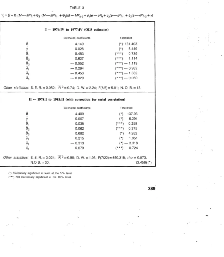
Equation (9) was tested for those two subperiods, with the lag structure being empirically determined. The estimates are reported in table 3 (6).
Table 3 shows that for the first of the two subperiods only the intercept and the time variable are statistically significant. Monetary surprises, where we include unanticipated changes in the exchange rate, have no real effects whatsoever. But from 1978:1 to 1985:11 the estimates tell quite a differente story; in addition to the intercept and the time variable, monetary shocks impact significantly upon real income as well. However, the impact of unan-ticipated money occurs with some delay. This variable is not statistically sig-nificant neither contemporaneously nor in the previous quarter, but it is both significant and positive two quarters in the past, as shown by
0
3. Thisbehavior might probably be explained by adjustment costs in labor input, most specially because Portuguese labor laws have been understood as quite res-trictive by actual and potential employers alike.
TABLE 3
I - 1974:IV to 1977:1V (OLS estimates)
Estimated coefficients
4.140 O.G28 0.483 0.627 -0.552 -0.264 -0.453 -0.020
!-statistics
(*) 131.403 (*) 5.449 (***) 0.739 (***) 1.114 (***)-1.119 (***)- 0.982 (***)- 1.382 (***)- 0.060
Other statistics: S. E. R. = 0.052; Ff2 = 0.74; D. W. = 2.24; F(7/5) = 5.91; N. 0. B.= 13.
II - 1978:1 to 1985:11 (with correction for serial correlation)
Estimated coefficients !-statistics
8
4.409 (*) 137.93y 0.007 (*) 6.291
01 0.038 (* **) 0.258
02 0.062 (* **) 0.375
03 0.682 (*) 4.282
J1 0.215 (*) 1.951
J2 -0.313 (*)- 3.318
J3 0.079 (* **) 0.724
Other statistics: S. E. R.
=
0.024; FF = 0.99; D. W. = 1.93; F(7/22) = 650.315; rho= 0.573;N.O.B. = 30. (3.456) (*)
Contemporaneous and one quarter in the past unanticipated changes in the exchange rate have also a significant impact on real income. Yet, while
3
1 conforms to the hypothesis, the same is not true with3
2. A tentativeexpla-nation for this apparently puzzling result requires not to focus on the labor mar-ket alone, as we have done so far, but to consider other marmar-kets' conditions as well, particularly the foreign exchange market. For most of that period, the US dollar appreciated considerably vis-a-vis most of the world's currencies, including the Portuguese escudo. At the same time, the Portuguese economy was unable to provide savers with attractive alternatives where to invest their excess liquitity; besides, businessmen lacked confidence in the national politi-cal and economic institutions, considerig that they were both characterized by a high degree of instability. Moreover, one could hardly find any investment as profitable and almost riskless as foreign exchange speculation, at a time when the US dollar was appreciating continuously. Indeed, it seems that for-eign exchange speculation reached very high amounts in those days. Follow-ing the explanation we propose, the negative estimate for d2 is picking-up the effects of speculators' forecast errors, in other words, when speculators real-ize that their one period ahead forecasts were inaccurate, they try do catch-up with events, which they do by revising their expectations and level of specula-tive engagement as well. For example, if e1.
1 turns out to be greater than e~ 1 ,
they exterpolate this outcome into the next quarter. As a result, speculation increses, and in the process productive resources are diverted away from real income producing activities. Implicitly, we have been asuming that Portuguese speculators(?) do not form their expectations rationally, but instead that they draw on their past experience according to some adaptive expectation mechanism.
It is evident that the model we have proposed performs differently, depend-ing on which subperiod we are considerdepend-ing. Its failure when usdepend-ing data from 1974:1V to 1977:1V might be due to the inherent abnormality of a revolutionary era more than to anything else. Additionally, the variance of money stock growth was much lower than in the following subperiod, i. e., 0.0026 versus 0.0036. This means that, in spite of everything else, the behavior of money was more predictable than it became latter on, which might also contribute to explain the different performances of the model.
We have performed a Chow test to validate or dismiss the assumption taken for granted up now that the whole sample period (1974:1V to 1985:11) was characterized by two different policy regimes. The test produced a F(8/27)
=
7.08, which is statistically significant at the 1 % level; accordingly, the initial assumption is fully validated.Bearing in mind the very high statistical significance of both the intercept and the time variable, we have looked at the joint significance of the remain-ing variables in the regression from 1978:1 to 1985:11. The null-hypothesis is that
0
1,0
2,
0
3,3
1,3
2 and3
3 are jointly zero. However, the computed F-test shows a value of F(6/22)=
10.47, which is also significant at the 1 % level, and in so being we reject the null-hypothesis. That is, this last result allows us to conclude that unanticipated monetary shocks do indeed matter in real income determination.IV -
Final remarksAll the tests undertaken have concurred on the idea that unexpected mone-tary shocks impact significantly upon real income, at least during the second of the time periods considered. The failure of the hypothesis formulated in equa-tion (9) to explain real income formaequa-tion from 1974:1V to 1977:1V might be due to a set of reasons, such as the inherent abnormality of a revolutionary period when the political, social and economic structures of a country are in the process of being deeply, and sometimes violently, transformed.
REFERENCES
BARRO, R. (1972), «Unanticipated money growth and employment in the US», American Economic Review, March.
(1978a), «Unanticipated money, output, and the price level in the United States>>, Journal of Political Economy, August.
(1978b), «Money and output in Mexico, Colombia and Brazil>>, in Jere, R. Behrman and J. Hanson (eds.).
BLEJER, M., and FERNANDEZ, R. (1980), «The effects of unanticipated money growth on prices and on output and its composition in a fixed-exchange-rate open economy>>, Canadian Jour-nal of Economics, February.
' BOSCHEN, J. (1985), «Employment and output effects of observed and unobserved monetary growth>>,
Journal of Money Credit and Banking, May.
FERNANDEZ, R. (1977), «An empirical inquiry on the short-run dinamics of output and prices>>, Ameri-can Economic Review, September.
GORDON, R. (1980), «Comment>>, in Rational Expectations and Economic Policy, edited by Stanley Fischer, University of Chicago Press, for N. B. E. R.
MISHKIN, F. (1982), «Does anticipated aggregate demand policy matter? Further economic results>>,
American Economic Review, September.
SMALL, D. (1979), «Unanticipated money growth and employment in the United States: Comment»,