Eduardo Barbosa Araújo
Scientific Collaboration Networks from Lattes
Database: Topology, Dynamics and Gender Statistics
Eduardo Barbosa Araújo
Scientific Collaboration Networks from Lattes Database:
Topology, Dynamics and Gender Statistics
Tese de Doutorado apresentada ao Programa de Pós-Graduação em Física da Universidade Federal do Ceará como requisito parcial para obtenção do título de Doutor em Física.
Área de Concentração: Física da Matéria Conden-sada.
Orientador: Prof. Dr. José Soares de Andrade Jr.
Trabalho aprovado. Fortaleza - Brazil, 25 de maio de 2016.
BANCA EXAMINADORA
Prof. Dr. José Soares de Andrade Jr.
(Orientador)
Universidade Federal do Ceará (UFC)
Prof. Dr. André Auto Moreira
Universidade Federal do Ceará (UFC)
Prof. Dr. Humberto de Andrade Carmona
Universidade Federal do Ceará (UFC)
Prof. Dr. Tarcísio Haroldo Cavalcante Pequeno
Universidade de Fotaleza (UNIFOR)
Profa. Dra. Suani Tavares Rubim de Pinho
Acknowledgements
Many persons, and institutions, were undoubtedly essential to the development of this thesis, not only on the practical aspects of the research undertaken but, and equally important, on the support given during these years. I could not thank these individuals enough and hope that I can somehow retribute their contributions in the future. Some of them I feel obliged to name. They are listed in the following. Those who I might forget, I ask to be forgiven and, next time you meet me, ask me for a drink.
Professor Dr. José Soares de Andrade Jr., for the opportunity of initiating this journey and, in this long path, for the many discussions, advice, helps and, more important, for your patience.
Professor Dr. André Auto Moreira, for all discussions and the opportunity of collaboration. Prof. Dr. Hans Jürgen Herrmann, for the opportunity of collaborating with your group at ETH-Zürich.
Luciano da Silva, Vasco Furtado, Tarcísio Pequeno and Nuno Araújo, for the works we did together.
Laura Barth, for the companionship, the motivation and the patience since the beginning of the Doctorate. I can not thank you enough.
The friends I met during these years: Saulo, Erneson, Hygor, Heitor, Rilder, Tatiana, Felipe, César, Rubens, Diego, Davi, Levi, Vagner, Vitor, Alexandre, Marcos (UFSC), Lineu (CBPF), Julian, Miller, Nicolas, Fahrang, Klara, Lucas, Gustavo, Amanda and Anabela.
My family.
The man who comes back through the Door in the Wall will never be quite the same as the man who went out. He will be wiser but less sure, happier but less self-satisfied, humbler in acknowledging his ignorance yet better equipped to understand the relationship of words to things, of systematic reasoning to the unfathomable mystery which it tries, forever vainly, to comprehend.
Resumo
Compreender a dinâmica de produção e colaboração em pesquisa pode revelar melhores estratégias para carreiras científicas, instituições acadêmicas e agências de fomento. Neste trabalho nós propo-mos o uso de uma grande e multidisciplinar base de currículos científicos brasileira, a Plataforma Lattes, para o estudo de padrões em pesquisa científica e colaborações. Esta base de dados in-clui informações detalhadas acerca de publicações e pesquisadores. Currículos individuais são en-viados pelos próprios pesquisadores de forma que a identificação de coautoria não é ambígua. Pesquisadores podem ser classificados por produção científica, localização geográfica e áreas de pesquisa. Nossos resultados mostram que a rede de colaborações científicas tem crescido exponen-cialmente nas últimas três décadas, com a distribuição do número de colaboradores por pesquisador se aproximando de uma lei de potência à medida que a rede evolui. Além disso, ambas a distribuição do número de colaboradores e a produção por pesquisador seguem o comportamento de leis de potência, independentemente da região ou áreas, sugerindo que um mesmo mecanismo univer-sal pode ser responsável pelo crescimento da rede e pela produtividade dos pesquisadores. Tam-bém mostramos que as redes de colaboração investigadas apresentam um típico comportamento assortativo, no qual pesquisadores de alto nível (com muitos colaboradores) tendem a colabo-rador com outros semelhantes. Em seguida, mostramos que homens preferem colaborar com outros homens enquanto mulheres são mais igualitárias ao estabelecer suas colaborações. Isso é consisten-temente observado em todas as áreas e é essencialmente independente do número de colaborações do pesquisador. A única exceção sendo a área de Engenharia, na qual este viés é claramente menos pronunciado para pesquisadores com muitas colaborações. Também mostramos que o número de colaborações segue o comportamento de leis de potência, com umcutoff dependente do gênero. Isso se reflete no fato de que em média mulheres produzem menos artigos e têm menos colabo-rações que homens. Também mostramos que ambos os gêneros exibem a mesma tendência quanto a colaborações interdisciplinares, exceto em Ciências Exatas e da Terra, nas quais mulheres tendo mais colaboradores são mais propensas a pesquisas interdisciplinares.
Abstract
Understanding the dynamics of research production and collaboration may reveal better strategies for scientific careers, academic institutions and funding agencies. Here we propose the use of a large and multidisciplinary database of scientific curricula in Brazil, namely, the Lattes Platform, to study patterns of scientific production and collaboration. Detailed information about publications and researchers is available in this database. Individual curricula are submitted by the researchers themselves so that co-authorship is unambiguous. Researchers can be evaluated by scientific pro-ductivity, geographical location and field of expertise. Our results show that the collaboration net-work is growing exponentially for the last three decades, with a distribution of number of collab-orators per researcher that approaches a power-law as the network gets older. Moreover, both the distributions of number of collaborators and production per researcher obey power-law behaviors, regardless of the geographical location or field, suggesting that the same universal mechanism might be responsible for network growth and productivity. We also show that the collaboration network under investigation displays a typical assortative mixing behavior, where teeming researchers (i.e., with high degree) tend to collaborate with others alike. Moreover, we discover that on average men prefer collaborating with other men than with women, while women are more egalitarian. This is consistently observed over all fields and essentially independent on the number of collaborators of the researcher. The solely exception is for engineering, where clearly this gender bias is less pro-nounced, when the number of collaborators increases. We also find that the distribution of number of collaborators follows a power-law, with a cut-off that is gender dependent. This reflects the fact that on average men produce more papers and have more collaborators than women. We also find that both genders display the same tendency towards interdisciplinary collaborations, except for Ex-act and Earth Sciences, where women having many collaborators are more open to interdisciplinary research.
Contents
1 INTRODUCTION . . . 23
2 NETWORKS . . . 26
2.1 Origins . . . 26
2.2 Elements and Types of Graphs . . . 26
2.3 Graph connectivity . . . 29
2.4 Representation of Graphs . . . 31
2.5 Properties of graphs . . . 33
2.6 Calculating paths . . . 34
2.7 Classical Random Graphs. . . 35
2.8 Barabási-Albert Model . . . 39
2.9 Small-world phenomenon . . . 39
2.10 Strogatz and Watts Model. . . 40
2.11 Random graphs with specified degree sequence . . . 41
3 LATTES COLLABORATION NETWORKS . . . 44
3.1 Scientific collaborations . . . 44
3.2 Co-authorship versus collaboration. . . 45
3.3 The network approach to scientific collaboration . . . 46
3.4 Lattes Platform . . . 47
3.5 Data acquisition and parsing . . . 48
3.6 Building a collaboration network . . . 52
3.7 The Total Collaboration Network. . . 53
3.8 Conclusions . . . 66
4 GENDER AND COLLABORATION . . . 68
4.1 Introduction . . . 68
4.2 Methods . . . 71
4.3 Results . . . 71
4.4 Conclusions . . . 78
5 CONCLUSIONS . . . 80
List of Figures
Figure 1 – The problem of the seven bridges of Königsberg. (a) The bridges connect land masses. It is asked if it is possible for one person to make a walk through the city while crossing each bridge once and only once. (b) Euler solved the prob-lem considering only the connectivity of the land masses. Considering the land masses points connected by lines representing the bridges, one can see that ex-cluding the starting and ending points, for each bridges to be crossed only once, the number of lines must be even: half are used to arrive at that land mass and half to leave it. Since all land masses are connected by an odd number of bridges, such walk is impossible. . . 26
Figure 2 – (a): An undirected graph G(V, E), with vertex set V = {1,2,3,4,5} and
edge set E = {(1,2),(1,5),(2,3),(2,4),(2,5),(3,4)}, which elements are
unordered pairs. Vertices 1 and 5 are adjacent since there is an edge(1,5)∈E.
Vertices 3 and 4 are the endpoints of the edge(3,4), and incident with this edge.
(b) A digraph G(V, E), where V = {1,2,3,4,5} and E = {⟨1,2⟩, ⟨1,5⟩, ⟨2,3⟩, ⟨2,4⟩, ⟨4,3⟩, ⟨5,2⟩}, which elements are ordered pairs. Arrows point
from the initial vertex of the edge to the final vertex. Vertex 1 is the initial ver-tex of the edge⟨1,5⟩, while vertex 5 is the final vertex of such edge. Note that
(a) is the undirected version of this graph. . . 27
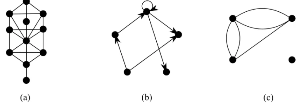
Figure 3 – Examples of graphs. (a): A simple undirected graph with 11 vertices and 17 edges. (b): A digraph with 5 vertices and 6 directed edges, one of them being a self-loop. Arrows point from initial vertex to final vertex. (c): A multigraph, in which there is more than one edge incident with the same pair of vertices. . . . 28
Figure 4 – A bipartite graph. Vertices can be partitioned into two disjoint sets, black circles and red squares. Edges must join vertices of different partitions. For example, for a citation network we may take squares as papers and circles as authors. Authors who are adjacent to a same paper are co-authors. . . 28
Figure 5 – Connectivity relationships on a digraphG(V, E). The correspondence (also called
neighbors) of vertices are:Γ(1) = {2,3}, Γ(2) = {3},Γ(3) = ∅,Γ(4) = ∅
andΓ(5) ={3,5}. The inverse correspondences are:Γ−1 =∅,Γ−1(2) ={1}, Γ−1(3) ={1,2,5},Γ−1(4) =∅andΓ−1(5) ={5}. The in-degree of vertices
are: δin(1) = 0, δin(2) = 1, δin(3) = 3, δin(4) = 0 andδin(5) = 1. The
out-degree of vertices are:δout(1) = 2,δout(2) = 1,δout(3) = 0,δout(4) = 0
andδout(5) = 1. The vertex 4 is isolated, sinceδin(4) =δout(4) = 0. . . . 30
Figure 6 – An undirected graph with 5 vertices and 7 edges. . . 32
Figure 7 – Particular random graphs obtained using theGN,pmodel withN = 20for
Figure 8 – Histogram of the degree distribution for aGN,pnetwork withN = 10000 and
p= 0.004. Dots represents the data points. The gray line is a fit using a Poisson
distribution (Eq. 2.24). The parameterz = 39.8898was obtained by maximum
likelihood estimation, close to the expected value for the average degree,39.996. 37
Figure 9 – G1000,prandom graph withpvarying from 0.00001 to 0.00500. Thus, the
aver-age degree of the networks varies from 0.001 to 5.00. For each value ofpwe
have built 10 different networks. The size of the giant component for each of these was obtained and the average value was taken for each value ofp. . . 38
Figure 10 – The Watts-Strogatz model [1]. We start with a regular lattice, here a ring lattice withN = 20vertices. Each vertex has degree 4, being adjacent to its nearest
neighbors and second-nearest neighbors. Initially, the graph displays high clus-tering and high average path length, l. For each edge there is a probability p
of changing one endpoint of the edge with the condition that we do not allow self-loops and multiple edges. The rewiring of edges creates shortcuts, causing
l to diminish. Ifp = 1we obtain a ER random graph, but with low clustering.
For intermediate values ofpthe graph displays both small average path length
and high degree of clustering. . . 41
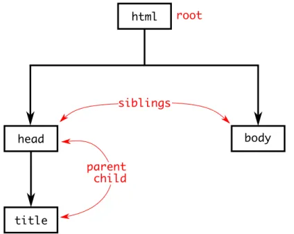
Figure 11 – Document tree of an xhtml document. <html> is the root element, with two children: <head> and <body>. <head> has a child <title>. . . 49
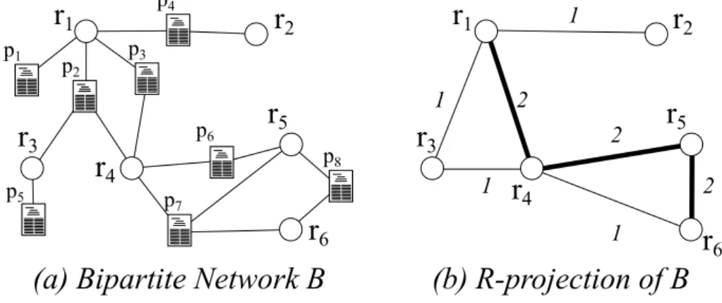
Figure 12 – (a) Bipartite networkBcontaining node classesRandPrepresenting researchers
(circles) and papers (rectangles), respectively. (b)R-projection ofB, where
re-searchers are connected if the share a paper inB. The weight of the link is given
by the number of shared papers. . . 52
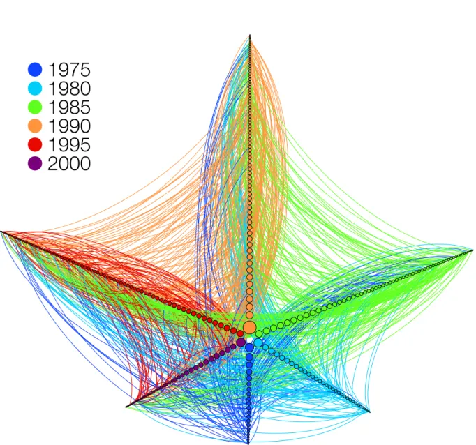
Figure 13 – Sample network extracted from the collected Lattes Database. Links shown are between researchers (nodes) who were granted a scholarship and working in fields of Medicine in the state of São Paulo. Node size is proportional to the degree of the researcher in the whole database. Researchers were grouped ac-cording to the year of their first published paper. The first cohort (dark blue) comprises all researchers who published their first paper before 1975. Each sub-sequent one, in the counterclockwise direction, comprises researchers who pub-lished within 5 years from the previous one, up to 2000. The edges are directed, colored according to the most senior. . . 54
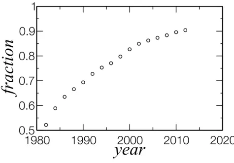
Figure 14 – Evolution of the fraction of the giant component of TCN since 1982. For every two years, the respective cumulative network was produced and the number of researchers in the largest component was divided by the number of researchers in collaboration in that year. . . 55
Figure 15 – Distribution of component sizessin the TCN, excluding the giant component.
Figure 16 – Left: Number of researchers with published papers (black circles) and collab-orations between them (red stars) present in the cumulative collaboration net-work. Dashed lines are exponential fits in the forms = aeαtup to 2009, seen
as straight lines in the linear-log plot. The coefficientαis shown in the picture
for each curve. Deviations of the 2012 data points from the exponential fit are due to the early acquisition of the curricula, in June of 2012. Right: Superlinear scaling of the number of collaborations with the number of researchers. Dashed line is a power-law curve with exponentαc/αr = 1.31. . . 57
Figure 17 – Evolution of the largest component. Data points represent the fraction of re-searchers present in the largest component for a five year time window centered in the respective year. More than 80% of the researchers engaged in collabora-tions in the last 5 years are in the largest component. They represent 61% of the researchers in TCN. . . 57
Figure 18 – Scaling ofC(k)withkfor the TCN (main graph) and the SCN (inset). The red
lines are power-law fits of the respective data (C(k) = Ak−σ). For the TCN,
σ = 0.71±0.009. For the SCNσ = 0.58±0.020. . . 59
Figure 19 – Distribution of scientific production of researchers belonging to the TCN group. The solid red line is the best fit to the data points of a power-law with exponential cutoff, P(n) = Apn−βpe−n/lp, whereβp = 1.58and lp = 129. The dashed
black line is a power-law with exponent−1.58. . . 60
Figure 20 – Normalized distribution of the number of collaborators (k) of researchers with
scholarship (blue stars), without (black circles) and for the TCN (red triangles). The distribution for researchers with scholarship decreases slowly up to one hundred collaborators, although most of them still have a small number of col-laborators. The higher proportion of researchers with high k might reflect the
CNPq policy of considering the proponent’s participation in research groups, international immersion and human resources development to grant the schol-arship. . . 61
Figure 21 – Variation of the average nearest-neighbor degree (knn) withk. Being an
increas-ing function of k, the network displays assortative mixing. Researchers with
high k are more likely to collaborate with other well connected researchers.
This tendency, however, increases logarithmically withk, as indicated by the
regression fit (dashed line). . . 61
Figure 22 – (a) Time evolution of the distribution of the number of collaborators in the TCN. (b) Rescaling the distribution in (a) by the relative number of collaborators for each year shows a collapse onto a single curve. We also show the respective cumulative distributions in (c) and (d). As the network ages, the fraction of re-searchers with highkincreases (c), but the evolution of the network shows that
Figure 23 – Interstate collaborations obtained from the Lattes Database. Vertices radii are proportional to the fraction of researchers in TCN. Edges are proportional to the total number of collaborations. Southeast states concentrate most of the collab-orations, specially São Paulo. . . 63
Figure 24 – Top: Distribution of number of collaborators in the TCN for the 26 Brazilian states and the Federal District. The distributions display the same behavior as the TCN (Fig. 22). The dashed line is guide for the eye in the form of a power-law with exponent 1.63 (P(k) =Ak−1.63). Bottom: the average number of
collab-orators versus the number of researchers in each state. The circles correspond to the results for 26 Brazilian states and the Federal District. The dashed line is the best fit obtained by linear regression of the data to a power-law⟨k⟩s∼ Nsδ
in logarithmic scale, with exponentδ= 0.12±0.01. . . 64
Figure 25 – Cumulative distributionsPCof the number of papers published per researchern
(a) and number of collaborators (b) for each of the 8 major fields. The respective distributions for the rescaled data are shown in (c) and (d). Lines represent dif-ferent fields, colored according to the symbol in the legend. Scientists working on social sciences and related fields (Lin, Soc and Hum) are less likely to have published more than one hundred papers than others. They also are less likely to have more than one hundred collaborators. Considering the average publica-tion count⟨n⟩f and average number of collaborations⟨k⟩f in each field, all the
curves collapse to a single universal behavior. The insets show the respective (non-cumulative) distributions. . . 65
Figure 26 – Study of interdisciplinary collaborations. Vertices represent different fields with sizes proportional to the fraction of collaborations with researchers of other fields. The directed edges are colored according to the source vertex and the width is proportional to the fraction of collaborations made with the target ver-tex. While some pairs are expected as Exa–Eng and Lin–Hum, the small frac-tions of collaborafrac-tions between researchers of Bio with Eng could indicate that biotechnology is still a maturing field. . . 67
Figure 27 – Average of the number of papers for male (blue bars) and female (red bars) researchers for the TCN and for each of the eight major fields: Agricultural Sci-ences (Agr), Applied Social SciSci-ences (Soc), Biological SciSci-ences (Bio), Exact and Earth Sciences (Exa), Humanities (Hum), Health Sciences (Hea), Engineer-ing (Eng) and LEngineer-inguistics and Arts (Lin). . . 71
Figure 29 – Top: number of male (blue squares) and female (red circles) researchers who published their first paper per year. It is clear that since 2000 women are the majority joining the collaboration network. In the bottom, we show the same data with the number of researchers in logarithmic scale, for better visualization of the transition point. . . 72
Figure 30 – a) Distribution of the number of recurrent collaborations (weights) between re-searchers, divided into male and female researchers. b) Distribution of the num-ber of collaborators, divided into male and female researchers. Women are less likely to display large values for both quantities. . . 74
Figure 31 – knnas a function of the number of collaborators (k) for male (blue squares) and
female (red circles) researchers. . . 75
Figure 32 – Fraction of new collaborators acquired as a function of time since the first pub-lished paper. Both male and female researchers display an exponential decay with a change in behavior occurring after 30 years. The dashed lines are expo-nential fits for the first 30 years:p(t) = Ae−λt. The calculated exponents are λw = 0.132±0.002for women andλm = 0.0998±0.001for men. . . 75
Figure 33 – Fraction of new collaborators who joined the collaboration network after the researcher, for men (blue squares) and women (red circles). While in the be-ginning of a researcher career most of his or her collaborators are older (i.e., joined the network before them), after only 5 years they display a balance be-tween older and younger collaborators. After 20 years of research, around 90% of new collaborators are younger and after 30 years, only a small fraction of new collaborators are older. The same behavior is observed for both genders. . . 76
Figure 34 – Mean values ofg-ratiofor each field of expertise: Agricultural Sciences (Agr), Applied Social Sciences (Soc), Biological Sciences (Bio), Exact and Earth Sci-ences (Exa), Humanities (Hum), Health SciSci-ences (Hea), Engineering (Eng) and Linguistics and Arts (Lin). Red and blue bars represent values for female and male researchers, respectively. Yellow triangles show the proportion of female researchers in the respective field. . . 77
List of Tables
Table 1 – Some relevant elements in the Lattes CV XML files and some corresponding attributes. . . 50
Table 2 – Cost and example of operations in Damereau-Levenshtein Algorithm implemen-tation used in this work. . . 53
Table 3 – Fraction of fields in the last 5 years. The network was constructed by projecting the bipartite network onto a network containing only researchers connected if they share a paper published in the last 5 years. Sum of fractions is not 100% because the field information is not available for all researchers. . . 56
Table 4 – Statistics for the networks studied in this work. . . 58
Table 5 – Statistics for researchers working on the 8 major fields associated with the TCN. 66
Table 6 – Number of male and female professors and researchers in Brazil. Source: Lattes Database (http://lattes.cnpq.br/), collected on 2015 January. . . 70
23
1 Introduction
Nowadays, scientific collaboration is understood as extremely valuable, as it integrates skills, knowledge, apparatus and resources, allows division of labor and the study of more difficult prob-lems, including interdisciplinary ones. It also brings recognition and visibility and increases the net-work of contacts of the researchers involved [2–4]. Scientific collaboration is strongly correlated with production measured by publication output and other indexes in Scientometrics [5–7], which has substantially contributed to raise the interest of the scientific community in studying itself over the last decades [3,5,8–11]. More recently, due to the fast growth and enormous development of the complex network science [1,12–22] the subject of scientific collaboration has been extensively studied under the framework of rather powerful and universal paradigms [23–29].
The Internet and the fact that traveling became substantially less costly have facilitated interna-tional collaborations. Still, geographical constraints affect the dynamics of research [30–32]. Differ-ent countries have differDiffer-ent funding policies and this fact impacts the publication outcome, which is correlated to collaboration. For a country to be above the world average number of citations, it must spend more than one hundred thousand US dollars per researcher per year [32]. At the same time, scientists with more investment in their research projects are more engaged in collaborations [33].
The social nature of collaboration [3,34] might be the cause for the big disparity in production and number of collaborators [35]. Inequalities in income (Pareto distribution [36]) and movie co-appearance [37] are examples of social distributions, characterized by a power-law profile. For scientific collaborations, such distributions also appear, as demonstrated by Lotka in 1926 [38], from the analysis of two empirical sets of publications data in natural sciences.
Although in Lotka’s analysis [38] only the senior authorship has been considered, the obtained power-law distributions was shown to be consistent with empirical bibliometric data taking all au-thors into account [39]. The so called Lotka’s Law therefore seems to be valid even in different fields than those originally considered [39,40]. It is also worth noting that highly prolific authors were excluded in Lotka’s procedure due to the limited number of persons in the samples. These teeming researchers might lie outside the pure power-law distribution. Considering that engaging in collaboration is a time consuming activity, the number of collaborators can not be arbitrarily large, i.e., must be somehow limited. An exponential cutoff has then been suggested as a correction to fit the distribution of productivity [27]. Measuring the distributions of citations by city or coun-try, a power-law distribution also arises [32], which indicates the presence of self-similarity in the science system [41].
ex-24 Chapter 1. Introduction
perimental work is usually rewarded with a co-authorship [4]. Also, analysing co-authorship makes it feasible to study collaboration of a greater number of researchers as compared by interviewing each individual.
Despite the numerous studies about scientific production, citations and collaborations found in the literature, it is difficult to compare these variables as the databases used in these studies are usually unrelated [42]. Another problem is the small number of samples, due to a low number of respondents in questionnaires or data used only from a specific journal. To analyse the big picture is paramount to work with a dense information database. Here, we used data from Lattes Platform (http://lattes.cnpq.br), an online database maintained by CNPq (National Council of Technological and Scientific Development), a government agency that finances scientific research in Brazil. It contains the curricula of almost all researchers in Brazil and some of their collaborators abroad, as well as information concerning their research groups. The Lattes Curriculum became the standard national scientific curriculum in Brazil, and compulsory for those requiring financial support from the Brazilian government. The curricula present detailed information concerning the researcher, in-cluding, but not limited to, full name, professional address, academic titles, field of expertise and list of papers. Researchers are classified in 9 major fields: Agricultural Sciences (Agr), Applied So-cial Sciences (Soc), Biological Sciences (Bio), Exact and Earth Sciences (Exa), Humanities (Hum), Health Sciences (Hea), Engineeing (Eng), Linguistics and Arts (Lin), Technologies1, and Others
(Oth). Most information in the curriculum is provided by the researcher themselves, for example, their list of publications.
By using this database, we may overcome some of the limitations found by other authors [23,24]. Due to the lack of individual information of the researcher, the problem of author name disambigua-tion [24,43] becomes relevant, when, for example, two or more authors share initials and surnames. This is not the case with the Lattes Platform, where co-authorship is unambiguous. Researchers themselves update their curricula with detailed information about their publications and profes-sional activity. As a consequence, this type of data allows us to study scientific production and collaborations of individual researchers and correlations between fields of expertise.
The science of networks is built upon the mathematical concept of graph. In physics, its ap-plication can be traced back to the works of Kirchhoff on electric circuits. Networks can be used as a model to study the dynamics of non-linear phenomena, as disease spreading [44–46] and the physics of the brain [47,48]. The technological advancement allowed scientists to study massive networks, a prohibitive task decades ago. This was facilitated not only by means of more powerful processors and greater data storages but also by the availability of high quality data and faster means of communication, in special the Internet.
The sequence of this work is as follows. In the second chapter we present the concept of graph and discuss different types of graphs. Following this, we summarize some concepts which are rel-evant for this work, such as degree, degree distribution, components of graphs, path length and
1 This field was recently included and was not available when this research was conducted. Hence, it will not be
25
clustering. We discuss real network properties and models, starting with the Erdős-Renyi random graph [49,50] and its inadequacy to describe real networks. We present the preferential attachment model [23], which reproduces the degree distribution observed in real networks. In the sequence, we discuss the small world phenomena [51] and a small-world model which incorporates clustering of vertices [1].
In the third chapter we give a review of works on scientific collaboration networks. We present the views on what consists a scientific collaboration and how collaboration networks are built. Af-terwards, we present findings which characterize scientific collaboration networks. We present the Lattes Platform as an object of study, discussing the extensive available information. Afterwards, we discuss our method of data mining and data storage for further processing. The construction of the networks are described. We discuss results on the collaboration network of the Lattes Plat-form. We investigate the evolution of the network, the differences and similarities between fields of expertise.
In the fourth chapter we characterize the general aspects, performance and differences between male and female researchers for different fields of expertise. We introduce two original metrics to investigate divergent behaviour of male and female researchers and show the existence of a gender bias, which is a relevant factor contributing to the underrepresentation of women in academy.
2 Networks
2.1 Origins
The study of networks is built upon the mathematical concept of graph, which had its inception in 1736 with a work of the Swiss mathematician Leonhard Euler (1707-1783). Euler presented the solution to the following problem: in Königsberg, Prussia (nowadays Kaliningrad, Russia), there was a river which surrounded an island and was divided into two branches, as shown in Fig.1. There were seven bridges crossing the river and connecting the land masses. Concerning these bridges, would it be possible to find a route crossing each bridge once and only once? Euler proved that this was impossible and his ingenious solution resulted in the birth of a new branch of mathematics.
2.2 Elements and Types of Graphs
A graph consists of a collection of elements which we call vertices (nodes, actors, site and
pointsare also used in the literature) whose relationships to one another are represented as edges
(orlinks,ties). Thus, we characterize a graphGby its sets of verticesV and edgesE asG(V, E).
This very broad concept allow us to use graphs to represent very different systems: the world
A
B
D C
(a)
A C
B
D
(b)
2.2. Elements and Types of Graphs 27
1
2
3 4
5
(a)
1
2
3 4
5
(b)
Figure 2 – (a): An undirected graph G(V, E), with vertex set V = {1,2,3,4,5} and edge set
E = {(1,2),(1,5),(2,3),(2,4),(2,5),(3,4)}, which elements are unordered pairs.
Vertices 1 and 5 are adjacent since there is an edge(1,5) ∈ E. Vertices 3 and 4 are
the endpoints of the edge(3,4), and incident with this edge. (b) A digraph G(V, E),
whereV ={1,2,3,4,5}andE ={⟨1,2⟩,⟨1,5⟩,⟨2,3⟩,⟨2,4⟩,⟨4,3⟩,⟨5,2⟩}, which
elements are ordered pairs. Arrows point from the initial vertex of the edge to the final vertex. Vertex 1 is the initial vertex of the edge⟨1,5⟩, while vertex 5 is the final vertex
of such edge. Note that (a) is the undirected version of this graph.
wide web (WWW) [52], the internet [53], actors networks [1,37], network of sexual contacts [54], products networks for recommendation systems, mobility [55], food webs [56], genetic networks, the brain [48,57], metabolic networks [58], evolution of diseases [59] and even networks of net-works [60]. Graphs can be pictorially represented as dots, symbolizing the vertices, and bars joining dots, symbolizing the edges.
Each edge has two vertices as itsendpointsand these are said to beadjacentto each other and
incidentwith this edge. The relationship expressed by the edge may have a directional quality. For example, due to the subjective concept of friendship, it is possible that a person considers another as his or her friend but this might not be reciprocal. In this case, we call the edges of the graphdirected
and the graph itself adirected graphordigraph. In a directed edge, we have aninitial vertexand afinal vertex. If there is no such directional property, we haveundirected edgesand anundirected graph. This is the case of co-authorship networks, when we consider that there is a link between co-authors of a paper. We represent the edges of a digraph as an ordered pair of vertices⟨v1, v2⟩, where v1 is the initial vertex andv2 the final vertex. For undirected graphs this pair is unordered and represented as(v1, v2).
28 Chapter 2. Networks
(a) (b) (c)
Figure 3 – Examples of graphs. (a): A simple undirected graph with 11 vertices and 17 edges. (b): A digraph with 5 vertices and 6 directed edges, one of them being a self-loop. Arrows point from initial vertex to final vertex. (c): A multigraph, in which there is more than one edge incident with the same pair of vertices.
Figure 4 – A bipartite graph. Vertices can be partitioned into two disjoint sets, black circles and red squares. Edges must join vertices of different partitions. For example, for a citation network we may take squares as papers and circles as authors. Authors who are adjacent to a same paper are co-authors.
at all is anempty graphand a graph with all possible edges is a complete graph: every vertex is adjacent to one another.
For all graphs considered until now, there is no conceptual correlation between edges and ver-tices. This is not the case for all possible graphs. For example, consider as vertices of a graph the students enrolled in disciplines and the disciplines themselves. Consider also that there is an edge between a student and a discipline if the student is enrolled in that specific discipline. We can see that in this case the graph will not have any edge between students or between disciplines. This is what we call abipartite graph. In bipartite graphs, we can partition the vertices into two disjoint sets such that there are no edges between elements belonging to the same partitioned set (see Fig.
2.3. Graph connectivity 29
We may generalize the definition of a graph including another setWof elements calledweights.
Weights are numbers which can be associated to vertices or edges of a graph, now denoted by
G(V, E, W). A graph with weights associated to edges is called anedge-weighted graph. Numbers
can also be associated to vertices, forming avertex-weighted graph. In this work we refer to edge-weighted graphs simply asweighted graphs. We call thestrengthof a vertexs(v)the sum of the
weightswiof the edges incident withv
s(v) =∑wi. (2.1)
2.3 Graph connectivity
We define thecorrespondenceΓ(v)of a vertexv in a digraphG(V, E)as the set
Γ(v) ={v′ ∈V|⟨v, v′⟩ ∈E}. (2.2)
For undirected graphs, the correspondence of a vertex is defined as the the correspondence of such vertex in the directed version of the graph. The correspondence of a set of vertices is defined as the union of the correspondence of each of those vertices,
Γ({v1, v2, . . . , vn}) = Γ(v1)
∪
Γ(v2)
∪
· · ·∪Γ(vn). (2.3)
Theinverse correspondenceΓ−1(v)of a vertexvin a digraphG(V, E)is the set
Γ−1(v) = {v′ ∈V|⟨v′, v⟩ ∈E}. (2.4)
For a vertex in an undirected graph, the inverse correspondence is obtained by computing its value for the directed version of the graph. For a set of vertices, the inverse correspondence is analogous to the correspondence,
Γ−1({v1, v2, . . . , vn}) = Γ−1(v1)
∪
Γ−1(v2)
∪
· · ·∪Γ−1(vn). (2.5)
We may apply the correspondence function successively and define
Γp(v) = Γ(Γp−1(v)), p∈N. (2.6)
The setΓ(v)is called theneighboring setofv and all its elements are calledneighborsofv. The
cardinality ofΓ(v)is called thedegreeof vertex1v,δ(v),
δ(v) =n(Γv). (2.7)
A vertex with δ(v) = 0 is called isolated (node 4in Fig. 5). For a digraph, a vertex v has two
degrees associated. Thein-degreeδin(v)is the number of edges withvas the final vertex,
30 Chapter 2. Networks
1
2
3
4 5
Figure 5 – Connectivity relationships on a digraph G(V, E). The correspondence (also called
neighbors) of vertices are: Γ(1) = {2,3}, Γ(2) = {3}, Γ(3) = ∅, Γ(4) = ∅
and Γ(5) = {3,5}. The inverse correspondences are: Γ−1 = ∅, Γ−1(2) = {1},
Γ−1(3) = {1,2,5}, Γ−1(4) = ∅ andΓ−1(5) = {5}. The in-degree of vertices are:
δin(1) = 0,δin(2) = 1, δin(3) = 3, δin(4) = 0andδin(5) = 1. The out-degree of vertices are:δout(1) = 2,δout(2) = 1,δout(3) = 0,δout(4) = 0andδout(5) = 1. The vertex 4 is isolated, sinceδin(4) =δout(4) = 0.
Theout-degreeδout(v)is the number of edges withv as the initial vertex
δout(v) =n(Γ(v)), (2.9)
see Fig.5.
Awalk in an undirected graph is a sequence of alternating vertices and edges, starting with a
source vertex and ending with atarget vertex, with each edge having as endpoints the adjacent vertices in the sequence. If the source and target vertices are the same, we have aclosed walk. A
trailis a walk in which each edge appears only once. Apathis a trail in which each vertex appears only once. A cycle is a closed trail in which all vertices but the source and target are distinct. A graph containing a cycle is acyclic graph. A graph with no cycle is anacyclic graphor aforest. We say that two vertices areconnectedon an undirected graph if there is a path with one of them as source and the other as target. An undirected graph in which all pairs of distinct vertices are connected is called aconnected graph. A connected forest is a tree. For digraphs, we define adirected-walk
as a sequence of vertices and directed edges in which the edges have as ending points the adjacent vertices in the sequence. Likewise, we definedirected-trails,directed-pathsanddirected-cycles
when the edges in sequence are directed.
The set of vertices for which there is a directed-path starting from a vertexvis the reachable set
of vertexv,R(v). If we have the correspondences of each vertex of a graphG(V, E),R(v)can be
found computing,
R(v) = {v}∪Γ(v)∪Γ2(v)· · ·∪ΓN(v), (2.10)
2.4. Representation of Graphs 31
where N = n(V)is the number of vertices in the graph. The set of vertices for which there is a
directed-path ending in a vertexv is the reaching set of vertexv,Q(v). If we have the
correspon-dences of each vertex of a graphG(V, E),R(v)can be found computing
Q(v) ={v}∪Γ−1(v)∪Γ−2(v)· · ·∪Γ−N(v), (2.11)
whereN =n(V)is the number of vertices in the graph.
We call a digraphstrongly-connected ifR(v) = V, ∀v ∈ V. If its underlying graph is
con-nected, we say that a digraph isweakly-connected. For an undirected graph, ifR(v) ̸=V for any v ∈V we call this adisconnected graph.
LetG(V, E)be a graph. If we takeV′ ⊆ V andE′ ⊆ E such that for every endpointv of e ∈E′,v ∈V′,G′(V′, E′)is asubgraphofG(V, E). IfG′ ̸=G, we sayG′is aproper subgraph
of G. For any disconnected graphG(V, E), we call componentsof G, the disjoint set of connect
subgraphs of G which are not contained in a connected subgraph with more vertices or edges.
For any digraph Gwe may consider the maximum subgraph G′ which is strongly connected.G′
is then called thestrongly-connected component ofG. In the same sense, we call theconnected
component of a graph G, the maximum subgraph of G which is weakly-connected. In network
science, this connected component may also be referred as the giant component or the largest component.
2.4 Representation of Graphs
Although a graphG(V, E)is completely defined by the setsV andE, there are more convenient
representations, specially when they are created and/or processed by computer programs. A suitable way of representing a graph G(V, E)is by an adjacency matrixA = [aij]. For a graph with n vertices (n(V) = n), this is a square n × n binary matrix which rows and columns represent
individual vertices and an elementaij is 1 if vertexiis adjacent to vertexj and 0 otherwise. More precisely, its elements are defined as
aij =
{
1 , ifj ∈Γ(i)
0 , ifj ∈/ Γ(i) (2.12)
For undirected graphs, this is a symmetric matrix and the sum of the elements of a line or column equals the degree of the respective vertex. Notice that this representation is equivalent to consider
32 Chapter 2. Networks 1 2 3 4 5 e1 e2 e3 e4 e5 e6 e7
Figure 6 – An undirected graph with 5 vertices and 7 edges.
As an example, consider the graph shown on Fig.6. Its adjacency matrixAis given by
A=
x1 x2 x3 x4 x5
x1 0 1 1 0 1
x2 1 0 0 1 1
x3 1 0 0 0 1
x4 0 1 0 0 1
x5 1 1 1 1 0
Another useful representation is by anincidence matrix. Considern(V) =nandn(E) =m.
The incidence matrix is an×mmatrix with rows representing the vertices and columns representing
the edges. For undirected graphs this is a binary matrix and an elementbij is 1 if vertexiis incident with edgejand 0 otherwise. For directed graphsbijcan be -1, 0 or 1, depending on whether vertex
iadjacent with edgej as a start vertex (1), end vertex (−1)or is not adjacent(0). The incident
matrix for the graph shown in Fig.6is
B =
e1 e2 e3 e4 e5 e6 e7
x1 1 1 1 0 0 0 0
x2 1 1 0 1 0 0 0
x3 0 1 0 0 0 1 0
x4 0 0 0 1 0 0 1
x5 0 1 1 1 0 1 1
These representations may become inefficient if the graph issparse: the number of edges on the graph is comparable to the number of vertices. In this case, the matrix representations contain many zeros, being computationally costly. A more common way of representing a graph is using anedges list, which uses2mdata units, wheremis the number of edges in the graph.
Other matrices of interest are the reachable matrix and reaching matrix. The former is defined as
Rij =
{
1 , ifj ∈R(i)
0 , ifj ∈/ R(i) (2.13)
and the latter
Qij =
{
1 , ifj ∈Q(i)
2.5. Properties of graphs 33
They represent all vertices that can be reached (reach) by paths starting (ending) on vertex i. For
undirected graphsR =Q. For a connected undirected graph all elements are 1. For disconnected
undirected graph, the matrices can be put in the form of a diagonal block matrix, where each block represents a connected component of the graph.
2.5 Properties of graphs
Thedegree distribution p(k)of a graph G(V, E)is defined as the number of vertices of V
which have degree equal tok,
p(k) = |{v ∈V|δ(v) = k}|. (2.15)
We can normalizep(k)and interpret it as the probability of randomly selecting a vertex with degree
k. The degree distribution is usually represented as a histogram. In some cases this histogram is
better visualized when displayed in a log-log scale, as for a power-law degree distribution.
The histogram of the degree distribution is a first step in network analysis, as the degree distribu-tion is related to the mechanism of network evoludistribu-tion. For a completely random network, where the probability of an edge to be present in the network is the same for all edges, the degree distribution follows a Poisson distribution [49], as it shall be demonstrated latter in this chapter. But in general the degree distributions for real networks seldomly display this behavior [61]. This deviation from the expected behavior for a random network provides evidence for an underlying mathematical structure governing the formation of edges.
For an undirected graphG(V, E), the shortest pathbetween two vertices v1, v2 ∈ V is the path fromv1to v2 with the least number of edges. The number of edges in the shortest path is the shortest path distance,d(v1, v2). It is possible that there are several paths with the same distanced. If verticesv1 andv2 are in different components,d(v1, v2) =∞. Theeccentricitye(v)of a vertex
v if defined as the maximum shortest distance fromv to any other vertex of the network,
e(v) =max
x∈V {d(v, x)}. (2.16)
Theradiusr(G)of a graphG(V, E)is the eccentricity of the vertex with lowest eccentricity in the
graph,
r(G) =min
v∈V e(v). (2.17)
Thediameterdiam(G)of a graphG(V, E)is the eccentricity of the vertex with largest eccentricity
in the graph,
diam(G) = max
v∈V e(v). (2.18)
The sum of the distances from a vertex to all other vertices in the network is calleddistance sum,
dsum(v) =∑u∈V d(v, u). An important statistical measure for graphG(V, E)is the average path lengthl,
l =
∑
v∈V dsum(v)
34 Chapter 2. Networks
wheren=n(V). Notice that in this definition we included the distance from a vertex to itself, which
is zero. Excluding these distances from the mean is equivalent to multiplyl by(n−1)/(n+ 1).
When the graph is disconnected, this definition leads to an infinitel. One solution is to consider only
paths with finite distance when computing the mean. This can be avoided by changing the average path length definition to the harmonic mean of the distance sums,
l−1 =
∑
v∈V d−sum1 (v)
n(n+ 1)/2 . (2.20)
Computing all-pair shortest paths for unweighted graphs can be done using a simple breadth-first search algorithm [62] (also known as ‘burning algorithm’ in physics), whereas for weighted graphs Dijkstra [63] or Bellman-Ford [64,65] algorithms give the desired metric.
The clustering coefficient C introduced by Watts and Strogatz [1] measures the likelihood
that an edge exists between two vertices connected to a given vertex. For example, it tell us the probability that two friends of a given person are also friends. It is defined as follows. Consider a vertexv of a graphG(V, E)with degreekv. Consider the subgraphV′ formed by v and itskv neighbors and all theneedgese∈Ebetween them. If this subgraph were complete, it would have
kn(kn−1)/2edges.Cv defined as the ratio of theneexisting edges and the total of the complete graph. The clustering coefficient is them the average ofCnover all vertices of the graph.
Another metric used in network analysis is theclustering coefficient c(v)of a vertex, defined
as
c(v) = number of triangles connected to vertexv
number of triples centered on vertexv . (2.21)
Note thatc(v)is ill-defined ifδ(v) = 0or 1. In this case, we setc(v) = 0. Hence, the clustering
coefficient of a graphCis
C = 1
n
∑
v∈V
c(v), (2.22)
wheren =n(V).
2.6 Calculating paths
There are several algorithms for calculating the distance between vertices on a graph. For un-weighted simple graphs, the breadth first search algorithm [62] can be used to calculate the average path distance, diameter and radius of the graph. For weighted graphs, Dijkstra algorithm [63] can be used for the task, when weights are positive. For network with negative, weights the Bellman-Ford algorithm [66] can be used.
The breadth first search algorithm calculates the distance from a source vertex to any other reachable vertex of the graph. This algorithm can also be used to determine the number of connected components of an undirected graph. By applying the algorithm for every vertex in the graph, we can calculate the average path lengthl.
2.7. Classical Random Graphs 35
Listing 2.1 – Pseudocode describing the breadth-first search algorithm.Gis a graph andG.V is the
vertex set ofG.sis the source vertex. Status is a vertex property with string values
unburnt, burning or burnt. Time is a vertex property given by an integer number. Parent is a vertex property indicating which adjacent vertex changed the status of the former. The shift operation remove the first element of a set.
f o r each v e r t e x u∈G.V− {s}
u . time = ∞
u . s t a t u s = ‘ u n b u r n t ’
␣u . p a r e n t␣=␣n i l s . s t a t u s␣=␣‘ b u r n i n g ’ s . time = 0
s . p a r e n t = n i l b u r n i n g = {s}
while b u r n i n g ̸={∅} u = b u r n i n g . s h i f t f o r each v i n Γ(u)
i f v . s t a t u s == ‘ u n b u r n t ’
␣␣␣v . s t a t u s␣==␣‘ b u r n i n g ’ v . time = u . time + 1 v . p a r e n t = u b u r n i n g << v u . s t a t u s = ‘ b u r n t ’
1. only unburnt trees can be ignited and become burning trees in the next time step;
2. at each time step, any burning tree ignites its adjacent unburnt trees and becomes burnt.
Hence, to calculate distances from any tree to a specific one (called the source), we consider that in the begining (t= 0) the source is burning and every other tree is unburnt. At each time step, we
increase the time by 1 and apply the rules above. The algorithm stops when there are no burning trees in the begining of the time step. The time in which a tree becomes burnt is the desired distance. The pseudocode describing the algorithm is given in Listing2.1.
2.7 Classical Random Graphs
The study of particular networks2may elucidate observed relatioships between topological and
dynamical variables of the systems represented. For example, it may help us to identify the most critical transmission lines in a power grid [67] or to how to minimize the effect of genetic disor-ders [68]. Nonetheless, in many situations we do not have knowledge of the complete topology of the systems under consideration. Furthermore, it is also interesting to study general properties of similar systems, which evolve based on the same underlying principle; however, due to randomness, they develop into different networks. Concerning these subjects is the study of random graphs. A random graph is not a specific graph obtained by a random procedure but a statistical ensemble of such graphs, each with some realization probability. This is similar to the concept of ensemble in statistical physics, where we obtain thermodynamical properties by averaging that property over all
2 From now on we will adopt the term network instead of graph when describing real systems, in order to emphasize
36 Chapter 2. Networks
p=0.00
(a)
p=0.15
(b)
p=0.30
(c)
p=1.00
(d)
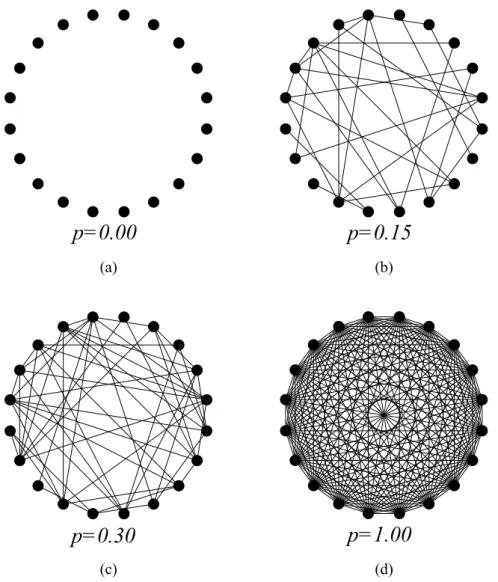
Figure 7 – Particular random graphs obtained using theGN,p model withN = 20 for different probabilitiesp: (a)p= 0.00, (b)p= 0.15, (c)p= 0.30and (d)p= 1.00.
the systems comprising the ensemble. Once we define our random graph we may obtain properties which are shared by a large fraction of the ensemble elements.
During the 1950s, the study of random graphs was undertaken by several authors. The first authors to consider this subject were Solomonoff and Rapoport [69,70]. The ensemble defined by them is known today as the Gilbert modelGN,p, due to Gilbert’s latter description of the model in 1959 [71]. In this model we have a set ofN vertices and a probabilitypthat any two vertices are
connected. To construct the ensemble elements, we start withN isolated vertices. For each pair of
vertices,vi andvj, we add an edge(vi, vj)to GN,pwith probability p. Thus, the existence of an edge is independent of any other. Using only these two parameters we form an ensemble of graphs. In Fig.7we show some random graphs obtained by different probabilitiesp.
By the end of the 1950’s, Erdős and Rényi rediscovered the random graphs [49,50], however, considering a different ensemble. Instead of considering a probabilityp, they studied all graphs with
self-2.7. Classical Random Graphs 37
0
20
40
60
k
0
0.01
0.02
0.03
0.04
0.05
0.06
0.07
p(k)
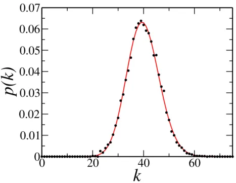
Figure 8 – Histogram of the degree distribution for aGN,pnetwork withN = 10000andp= 0.004. Dots represents the data points. The gray line is a fit using a Poisson distribution (Eq.
2.24). The parameter z = 39.8898 was obtained by maximum likelihood estimation,
close to the expected value for the average degree,39.996.
loops, which are not present in theGN,pmodel. Although these models are conceptually different, in the limit of large sparse graphs the difference can be neglected. Thus, in the following we shall discuss properties of theGN,pmodel.
For each vertex inGN,pthere areN −1vertices to which it may be connected by an edge. Let us consider a vertexv with degreeδ(v) = k. There are(n−k1) ways of connectingv to the other
vertices. Meanwhile the probability of v to be connected to exactly k other vertices is given by pk(1−p)n−1−k. Therefore, the probability distribution of degrees in the network is given by
P[δ(v) =k] =
(
n−1
k
)
pk(1−p)n−1−k, (2.23)
which is the binomial distribution. The average degree for such distribution is z = p(n−1). In
the limit of largeN while keepingzconstant, this distribution can be approximated by the Poisson
distribution,
P(k) = e
−zzk
k! . (2.24)
Figure8shows the degree distribution for a network with 10000 vertices andp= 0.004.
Consider a vertexvin aGN,prandom graph. Letkbe the degree ofv. The number of triangles containing v is (k2). The number of actual edges between neighbors of v isp(k2). Thus, c(v) =
p(k2)/(k 2
)
38 Chapter 2. Networks
0
1
2
3
4
5
〈
z
〉
0
200
400
600
800
1000
S
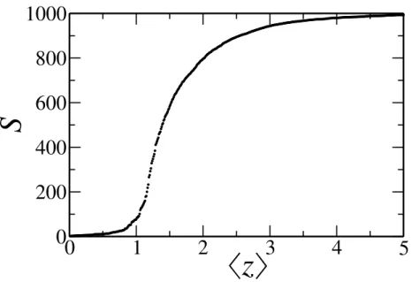
Figure 9 – G1000,prandom graph withpvarying from 0.00001 to 0.00500. Thus, the average degree of the networks varies from 0.001 to 5.00. For each value ofpwe have built 10 different
networks. The size of the giant component for each of these was obtained and the average value was taken for each value ofp.
graph. Hence,C is also equal top. Hence, GN,p random graphs with a small linking probability also display a small degree of clustering.
The most striking result concerningGN,prandom graphs is the emergence of a giant component. For small value ofpthe graph is disconnected, consisting of several small connected components.
There is a critical value ofpfor which there is a non-zero probability for any given vertex to belong
to this giant component. This critical value marks a phase transition from a low-density state, with many small components, to a high-density state with a very large component containing most of the vertices of the graph and the remaining vertices grouped in very small components. The critical value for this phase transition isp = z/(N −1)[14]. For largeN, this is equivalent toz = 1.
Hence, we have the following behavior, depending on the value ofz. Forz < 1, there are only
small components, the largest with sizes=O(lnn). Atz = 1, we have a critical point marking the
emergence of a giant component with sizes=O(N2/3). At this point, the cluster size distribution follows a power-law with exponent5/2. Finally, forz > 1, there is a giant component with size
O(N). The second largest component has sizes=O(lnn).
Figure9shows the emergence of the giant component. We have builtG1000,p random graphs withpvarying from 0.00001 to 0.00500. Thus, the average degree of the networks varies from 0.001
to 5.00. For each value ofpwe have built 10 different networks. The size of the giant component
2.8. Barabási-Albert Model 39
The average path length for ER random graphs is given by [72]
l = lnN −γ
lnz +
1
2, (2.25)
where γ is the Euler-Mascheroni constant (γ ≈ 0.5772). We see that the average path length
in-creases slowly, namely, with the logarithm of the size of the graph. As a result, even for large networks, vertices are at a small distance from each other.
2.8 Barabási-Albert Model
The degree distribution of real networks does not follow that observed in ER networks. More-over, many real networks display a heavy-tailed degree distribution, which in some cases, agrees with a power-law distribution [61]. Such networks are known asscale-free networks.
In a seminal 1999 paper [52], Barabási and Albert studied the degree distribution of networks of actors, the world wide web (WWW) and the power-grid network. They found that these distributions were better represented by a power-law, instead of a Poisson distribution. In order to understand why different systems as these give rise to a similar behavior, they proposed a model today known as the Barabási-Albert (BA) Model, composed of two ingredients:
1. The networks evolve continuously by the addition of new vertices. This is not the case for the ERGN,pmodel in which the number of vertices is fixed from the beginning and unrelated to the formation of edges.
2. When new vertices are added, they are linked preferentially to vertices with a high degree.
Barabási and Albert [52] have shown through computational simulation that, by following these simple rules, a power-law degree distribution is obtained, with exponent 2.9. Real scale-free net-works exhibit diverse exponents; nonetheless modifications of the BA model can produce different values. One distinctive feature of scale-free networks is the existence of hubs, namely, vertices with a very high degree. This is not observed in Poisson or Gaussian degree distributions due to their fast decrease for values distant from their mean. This feature is preserved by power-law distributions, which decay slowly compared to the former ones. Although successful in identifying a mathemat-ical structure leading to observed degree distribution, the BA model fails to produce the clustering observed in social networks.
2.9 Small-world phenomenon
40 Chapter 2. Networks
that the distance between any two persons in this network is awkwardly small. In the network of our society, everyone would be close to a movie start, to a politician or, even more surprisingly, to an undistinguished factory worker living in the suburb.
By the 1960’s, there were two views on this matter. First it was believed that the small-world phenomenon was true for our society and everyone would be close, as stated in the last paragraph. The second view considered that it was also true but that not every pair of persons would have a path between them: people would be close to the ones in their community, but people from other communities could not be linked. In other words, in this view, the network of the society did not form a connected network: each connected component would be a community, isolated from each other.
In 1967, Stanley Milgram carried out an experiment to investigate the possibility of studying the small-world phenomenon [51]. The experiment consisted in asking subjects, sampled from men and women from all walks of life, to deliver a letter to a target person living somewhere in the United States. If the person did not know the target on a first-name basis, he or she was asked to send to one of his or her acquaintances which, by their judgment, were the most likely to know the target on a personal basis, with the same instructions. Along with the letter there was a roster on which everyone who received the letter should write his or her name down. This allowed tracking the number of persons the letter passed through until it was delivered to the target. As a side effect, it would also prevent the letter to loop around a group of acquaintances.
The result of the experiment was startling: the median of intermediate acquaintances for the letter to reach the target person was only five. Thus, between those persons there were six links, giving origin to the now widely known expression ‘six degrees of separation’. Even the following criticism on the poor statistics and low response rate of the experiment did not reduce the importance of the work. Recently, the experiment was reproduced using e-mail instead of letters [73]. More than 60,000 e-mails users were asked to attempt to reach 18 target persons in 13 countries. The 348 completed tasks have an average of only 4.05 links.
2.10 Strogatz and Watts Model
The small-world phenomenon is not exclusive to the network of acquaintances. Many real net-works exhibit a rather small average path length, which is linked to clustering of vertices: there is a high probability that neighbors of a vertex have an edge between them as compared to a random graph as the ER model. This is measured by the clustering coefficient, which for ER graphs is equal to the probability of two vertices sharing an edge,p. When modeling real networks, this value must
be usually small, since it is related to the average degree of the networkz = p(N −1). Thus, ER
graphs, although having a small average path length, do not reproduce the clustering observed in the real world. Nonetheless, clustering is not a sufficient condition to produce a small-world network. Regular lattices are highly clustered while exhibiting a high average path length.
2.11. Random graphs with specified degree sequence 41
p=0
p=1
increasing randomness
Figure 10 – The Watts-Strogatz model [1]. We start with a regular lattice, here a ring lattice with
N = 20vertices. Each vertex has degree 4, being adjacent to its nearest neighbors and
second-nearest neighbors. Initially, the graph displays high clustering and high average path length,l. For each edge there is a probabilitypof changing one endpoint of the edge
with the condition that we do not allow self-loops and multiple edges. The rewiring of edges creates shortcuts, causinglto diminish. Ifp= 1we obtain a ER random graph,
but with low clustering. For intermediate values of p the graph displays both small
average path length and high degree of clustering.
networks [1]. Starting from a clustered regular lattice, the disorder observed in random networks can be obtained by rewiring some edges, changing one of the endpoints. This procedure, while keeping the clustering of the network, creates shortcuts between distant vertices on the original lattice, shrinking the average path length.
Consider a ring lattice, withnvertices and each vertex withkedges. Each edge has a probability pof being rewired at random. Thepparameter acts as a controller for a continuous phase transition
from an ordered state (p= 0) to an ER random graph (p= 1).
We show in Fig.10a ring lattice withN = 20vertices. Each vertex has degree 4, being adjacent
to its nearest neighbors and second-nearest neighbors. Forp= 0, the graph displays high clustering
and high average path length,l. With probabilityp, we change one endpoint of each edge (but not
allowing self-loops and multiple edges). This rewiring procedure creates shortcuts between vertices in the graph, diminishingl. Forp= 1the WS model reproduces the ER model, which displays low
clustering. The parameterpcan be ajusted for the obtained graph to exhibit high clustering and low l.
2.11 Random graphs with specified degree sequence
42 Chapter 2. Networks
It is possible to generate graphs which do not follow the preceding degree distributions, but any desiredpk. This can be done by working with a specific degree sequence{ki}, i = 1, . . . , n, wherenis the number of vertices in the network, chosen in such a way that the number of vertices
with degree k tends topk in the limit of large n [75]. Such degree sequence can be obtained by numerically drawing random numbers frompk.
The process to obtain a network can be pictured as giving sticks to the n vertices according
to the degree sequence. Then, we chose two sticks uniformly at random and add an edge to the vertices owing them. Notice that this procedure allows self-loops. Also, the sum of the terms in the degree sequence generated must be even. This procedure defines an ensemble of graphs with degree distributionpk.
Some properties of this model can be obtained in the limit of largen. In order to study the size
of the largest component, we must focus our attention to the number of neighbors of a vertex at a specific distance. The average degree of the first neighbors of a vertex isz = ⟨k⟩. For second
neighbors, we should in general subtract the average number of neighbors at distance 2 which are also at distance 1 from the vertex. In other words, we should take into account the clustering of vertices. However, we shall consider that the probability of two neighbors of a vertex to be joined by an edge goes asn−1.
Now, to find out the average number of second neighbors, we must consider the degree distri-bution of a vertex reached by following an edge. This is notpksince it is more likely that such edge belongs to a vertex with high degree. The actual distribution iskpk. Furthermore, the edge we used to reach that vertex leads back to the former, hence not increasing its number of second neighbors. Thus, we are interested in the remaining degree distribution of a vertex reached by following an edge,qk. The normalized distribution is
qk =
(k+ 1)pk+1
∑
jjpj
. (2.26)
The average degree of this vertex is
∞
∑
k=0
kqk =
∑∞
k=0k(k+ 1)pk+1
∑
jjpj
=
∑∞
k=0k(k−1)pk
∑
jjpj
= ⟨k
2⟩ − ⟨k⟩
⟨k⟩ . (2.27)
Multiplying this second neighbor average degree by the average number of first neighbors we obtain the average number of second neighbors,z2,
z2 =⟨k2⟩ − ⟨k⟩. (2.28)
We can repeat this procedure for more distant neighbors, obtaining the following expression for the number of neighbors at distancem,
zm =
⟨k2⟩ − ⟨k⟩
⟨k⟩ zm−1 =
z2
z1
zm−1 =
(
z2
z1
)m−1
z1. (2.29)
2.11. Random graphs with specified degree sequence 43
giant component do not exist (notice that we are considering the limit of infinite n). Thus, the
network exhibits a phase transition at the point wherez2 =z1. This condition can be rewritten as
⟨k2⟩ −2⟨k⟩= 0or
∞
∑
k=0
k(k−2)pk= 0, (2.30)
known as Molloy-Reed criterion for the existence of a giant component [76].
Thus, the presence of a giant component is not unique to classical random graphs but expected for arbitrary degree distributions as long as the Molloy-Reed criterion is satisfied. Notice that if
z2/z1 ≫1, most of the vertices in the giant component will be away from a specific vertexv. Since they outnumber the immediate neighborhood of v, the average path lengthlto vis approximately
the distance to these peripheral vertices. Settingzl≈n, we obtain
l ≈ ln(n/z1)
ln(z2/z1)
+ 1. (2.31)
For example, for an ER graph, we have
z1 =z, (2.32)
z2 =⟨k2⟩ − ⟨k⟩=z2. (2.33)
Then, in the limit of largenwe havel≈ln(n)/ln(z), which agrees with the exact result (Eq.2.25).

![Figure 10 – The Watts-Strogatz model [1]. We start with a regular lattice, here a ring lattice with N = 20 vertices](https://thumb-eu.123doks.com/thumbv2/123dok_br/15275988.542035/43.892.221.714.145.357/figure-watts-strogatz-model-regular-lattice-lattice-vertices.webp)