Atmos. Chem. Phys., 15, 7369–7389, 2015 www.atmos-chem-phys.net/15/7369/2015/ doi:10.5194/acp-15-7369-2015
© Author(s) 2015. CC Attribution 3.0 License.
Large-eddy simulation of contrail evolution in the vortex phase and
its interaction with atmospheric turbulence
J. Picot1, R. Paoli1, O. Thouron1, and D. Cariolle1,2
1CNRS/CERFACS, URA 1875, Sciences de l’Univers au CERFACS, Toulouse, France 2Météo France, Toulouse, France
Correspondence to:R. Paoli ([email protected])
Received: 07 October 2014 – Published in Atmos. Chem. Phys. Discuss.: 28 November 2014 Revised: 13 May 2015 – Accepted: 29 May 2015 – Published: 09 July 2015
Abstract.In this work, the evolution of contrails in the vor-tex and dissipation regimes is studied by means of fully three-dimensional large-eddy simulation (LES) coupled to a Lagrangian particle tracking method to treat the ice phase. In this paper, fine-scale atmospheric turbulence is generated and sustained by means of a stochastic forcing that mimics the properties of stably stratified turbulent flows as those oc-curring in the upper troposphere and lower stratosphere. The initial flow field is composed of the turbulent background flow and a wake flow obtained from separate LES of the jet regime. Atmospheric turbulence is the main driver of the wake instability and the structure of the resulting wake is sensitive to the intensity of the perturbations, primarily in the vertical direction. A stronger turbulence accelerates the onset of the instability, which results in shorter contrail de-scent and more effective mixing in the interior of the plume. However, the self-induced turbulence that is produced in the wake after the vortex breakup dominates over background turbulence until the end of the vortex regime and controls the mixing with ambient air. This results in mean microphysi-cal characteristics such as ice mass and optimicrophysi-cal depth that are slightly affected by the intensity of atmospheric turbulence. However, the background humidity and temperature have a first-order effect on the survival of ice crystals and particle size distribution, which is in line with recent studies.
1 Introduction
Aircraft-induced cloudiness in the form of condensation trails (contrails) and contrail cirrus is among the most uncer-tain contributors to the Earth radiative forcing from aviation (Lee et al., 2009). One of the main reasons of this uncer-tainty is the large disparity of scales that exists between the near field of aircraft engines, where emissions are produced, and the grid boxes of global models that are used to evaluate their global atmospheric impact (Burkhardt et al., 2010). In order to bridge this gap and develop more refined parame-terizations of unresolved plume processes into global mod-els, one has to gain better knowledge of the dynamical and the microphysical properties of contrails and their precursors. For that purpose, high-fidelity numerical simulations such as large-eddy simulations (LES) are now becoming a reliable instrument of research in the atmospheric science community as they allow for accurate description of the physicochemi-cal processes that occur in aircraft wakes (Unterstrasser and Gierens, 2010a; Paugam et al., 2010; Naiman et al., 2011).
even-tually leads to the formation of an upward-moving secondary wake (Spalart, 1996), where part of the exhausts and ice par-ticles are detrained (Gerz and Ehret, 1997). The vortices also interact with each other via a kinematic process of mutual in-stability (Crow, 1970; Widnall et al., 1974) until they break up and release the exhaust in the atmosphere (dissipation regime). For high ambient humidity, ice particle size can in-crease dramatically by condensation of ambient water vapor (Lewellen and Lewellen, 2001; Paugam et al., 2010; Naiman et al., 2011). During the final diffusion regime, the contrail evolution is controlled by atmospheric motion via shear and turbulence (Gerz et al., 1998) and by radiative transfer pro-cesses and sedimentation (Unterstrasser and Gierens, 2010a, b) until complete mixing, which is usually within a few hours.
From a computational perspective, the vortex regime is particularly challenging because of the intricate transforma-tions that occur in the wake and changes in the flow topol-ogy, which manifest as abrupt expansions of the contrail in both horizontal and vertical directions (Sussmann, 1999). These transformations necessarily affect the ice microphys-ical properties. Most numermicrophys-ical simulations of contrails in the vortex regime in the literature rely on Eulerian formula-tions for the treatment of ice particles. For example, Lewellen and Lewellen (2001), Huebsch and Lewellen (2006), and Paugam et al. (2010) used three-dimensional LES with dif-ferent levels of sophistication of ice microphysics, difdif-ferent setups of the dynamics, and different resolutions to cover timescales beyond the end of the vortex regime. The re-sults of these studies showed that ambient humidity, strat-ification, and turbulence are among the factors controlling the survival of ice crystals and their spatial distribution at the end of the vortex regime. These findings have been con-firmed by LES coupled to a Lagrangian particle tracking (LPT) method in three-dimensional (Naiman et al., 2011) and two-dimensional frameworks (Unterstrasser and Sölch, 2010). The latter authors also compared the results obtained with Eulerian- and Lagrangian-based methods on the same computational grid and observed that the LPT allows for a more accurate representation of ice microphysics. This as-pect was recently investigated by Unterstrasser et al. (2014) in the context of tracer dispersion in aircraft wake vortices. They observed that LPT appears to be less dissipative than Eulerian formulations in reproducing particle dispersion in aircraft wake vortices, although the details depend on the ac-curacy of the numerical scheme and the computational grid.
The dynamics of aircraft wake vortices have been studied traditionally in the wake vortex community for wake hazard applications. (The reader is invited to consult the reviews by Spalart, 1998; Gerz et al., 2002; Holzäpfel et al., 2003, and references therein for further details on this subject). The in-teraction between wake vortices, turbulence, and tracer dis-persion has been studied in the past by Gerz and Holzäpfel (1999) and more recently by Misaka et al. (2012), who
ana-lyzed the fine-scale dynamics and the mixing of exhaust trac-ers with ambient air.
An aspect that has not been fully investigated so far is the role of atmospheric turbulence in determining the three-dimensional structure of contrails and the ice microphysi-cal properties. For example, it is likely that turbulence en-hances the mixing of ice crystals with atmospheric water va-por, especially in the secondary wake, and it influences the detrainment of exhausts at the vortex boundaries. In addition, vortex instabilities such as Crow instability (Crow, 1970) or elliptical instability (Widnall et al., 1974) can be triggered by atmospheric turbulence, which ultimately leads to their breakup and decay. Unterstrasser et al. (2008) used two-dimensional LES with modified diffusion of the vortex core to mimic the effects of three-dimensional vortex decay in a turbulent environment, a procedure that was also used by Un-terstrasser and Gierens (2010a) and UnUn-terstrasser and Sölch (2010). Lewellen et al. (2014) recently proposed a “quasi-three-dimensional” approach which consists in resolving a certain narrow axial range of three-dimensional eddies that are imposed a priori rather than emerging naturally from the turbulent cascade. Comparisons of mean contrail parameters with those obtained using full three-dimensional LES were reported to be satisfactory for selected case studies. While the procedures described above are fast and suitable for sen-sitivity analysis of mean contrail properties to background turbulence, the treatment of vortex dynamics and the repre-sentation of atmospheric turbulence remain strongly param-eterized. In fully three-dimensional LES of contrail realized to date, turbulence models have been mainly used to trig-ger vortex instabilities rather than investigate the effects of background turbulence on the wake structure and the contrail properties. Paugam et al. (2010) introduced rather idealized perturbations in the form of sine waves, while Naiman et al. (2011), Lewellen et al. (2014), and Unterstrasser (2014) used divergence-free random fields with imposed spectra which are evolved in order to develop coherent turbulent eddies that constitute the initial condition for the contrail simulations. However, during this transient time turbulence decays, which makes it difficult to control the level of the atmospheric tur-bulence that effectively interacts with the wake vortices.
J. Picot et al.: LES of contrails in atmospheric turbulence 7371 and was specially devised for strongly stratified turbulent
flows such as those occurring in the upper troposphere and lower stratosphere (UTLS) (Paoli and Shariff, 2009; Paoli et al., 2014). To the authors’ knowledge, this is the first time such sophisticated treatment of atmospheric turbulence is employed for contrail simulations. This point is crucial to have a correct representation of turbulence that is strongly anisotropic and hence substantially different and more com-plex than classical Kolmogorov turbulence. The application of the forcing technique to the UTLS turbulence is described in the LES by Paoli et al. (2014), who analyzed and com-pared the statistical proprieties with theoretical analysis of strongly stratified flows (Brethouwer et al., 2007). The study showed that a substantial amount of turbulent kinetic energy is present at sub-kilometer scales relevant to the wake flow dynamics, which are then properly resolved. In particular, the LES data revealed the typical flow structures character-ized by horizontally layered eddies or “pancakes” (Riley and Lelong, 2000) that are a signature of the background field used for the present contrail simulations.
Although full unsteady spatial simulations of wake for-mation including the exhaust jets would help understanding the details of ice nucleation in rapidly changing thermody-namic conditions, they have not been performed so far as they would require far higher resolution and computational re-sources that are hardly available on present supercomputers. Hence, for the present study, the initial wake-flow field was reconstructed using data from temporal LES of the jet regime at a wake age of 10 s that takes into account the jet/vortex interaction process (Paoli et al., 2013) In addition, the nu-merical model uses a fully three-dimensional Lagrangian ap-proach to track the crystals. Since turbulence can be fully controlled, this methodology allows for a sensitivity analy-sis of the wake and contrail properties in the vortex regime as a function of turbulence intensity. The sensitivity to back-ground humidity and temperature is also discussed and com-pared to the sensitivity to turbulence.
The paper is organized as follows: Sect. 2 summarizes the model equations, Sect. 3 describes computational setup of the simulations, and Sect. 4 presents the results of the simu-lations. Conclusions are drawn in Sect. 5.
2 Model equations
The computational model used in this work is based on an Eulerian–Lagrangian approach: the large-scale eddies of the gaseous atmosphere are solved with compressible Navier– Stokes equations, while ice crystals are treated by a La-grangian tracking method and mass transfer between the two phases. As this model has already been presented else-where (Paoli et al., 2008, 2013), only a summary is presented here. The densityρ, velocityu, total energyE=CvT+12u2 (whereT is the temperature), and water vapor mass fraction
Yvare solution of the Favre-filtered Navier–Stokes equations: ∂ρ
∂t + ∇ ·(ρu)=ωv, (1a)
∂ρu
∂t + ∇ ·(ρu⊗u)+ ∇p=∇ ·T+ρg, (1b) ∂·ρE
∂t + ∇ ·((ρE+p)u)=∇ ·(Tu)+ρg·u− ∇ ·q, (1c) ∂ρYv
∂t + ∇ ·(ρYvu)= − ∇ ·ξ+ωv, (1d) where the source term ωv in Eq. (1a) and (1d) represents the mass transfer between vapor and ice phases detailed in Sect. 2.1; the tensor T=2µS−13Skk1
is the shear stress withS=12(∇u+ ∇u⊺),µ=µ
mol+µsgs, whereµmol and µsgs are, respectively, the molecular viscosity of air (mol) and the subgrid-scale (sgs) viscosity (the latter ob-tained from the filtered structure function model by Ducros et al., 1996); the vector g is the gravitational accelera-tion; the pressure p is obtained from the perfect gas law p=ρRT with R the gas constant for air; and the vectors q=qmol+qsgs and ξ=ξmol+ξsgs are the heat and va-por diffusion fluxes, respectively, each one composed of the molecular and sgs fluxes. Given the high Reynolds number flows considered in this study, the molecular transport are small compared to the turbulent transport, so that in prac-ticeµ≃µsgs,q≃qsgsandξ≃ξsgs. These are related to the gradient of temperature and vapor mass fraction by means of turbulent Prandtl and Schmidt numbers:qsgs= −Cpµ
sgs Prt ∇T andξsgs= −
µsgs
Sct ∇Yv. For typical atmospheric flows,P rand Scdepend on Richardson number and other atmospheric pa-rameters (see, e.g., Schumann and Gerz, 1995); however, at the resolution of O(1 m)considered here (see Table 1) the subgrid-scale turbulence can be considered isotropic (the Ozmidov scale in the UTLS is 1 order of magnitude larger; see, e.g., Brethouwer et al., 2007) and they are taken con-stant with valuesPrt=Sct=0.419 as in Gerz and Holzäpfel (1999).
Equation (1) are discretized on collocated, Cartesian meshes with non-uniform grid spacing. The spatial deriva-tives are computed with a sixth-order compact scheme refor-mulated for stretched grids (Lele, 1992; Gamet et al., 1999). A high-order selective artificial dissipation (Tam and Webb, 1993; Tam et al., 1993) was used to enforce numerical sta-bility while retaining the sixth-order spectral-like resolution at the resolved scales (see Barone, 2003 for details). Finally, time integration is performed by a third-order Runge–Kutta method with a Courant–Friedrichs–Lewy number fixed to CFL=0.5.
2.1 Ice model
ice forms by deposition of water vapor. Given the large soot emission index EIs=O(1015)kg−1(Kärcher and Yu, 2009), it would be prohibitive to track all soot particles in the wake, so only a reduced number of numerical particles are tracked by the model. A numerical particle represents a cluster of nc=n/np (identical) physical particles that have massmp, center of massxp, and velocityup. As particles remain small compared to flows structures, the point-force approximation (Boivin et al., 1998) can be used for particle-flow interac-tions, which means that all fluid properties at particle posi-tion are obtained through an interpolaposi-tion of the values at neighborhood grid points:
dxp
dt =up, p=1, . . ., np, (2a)
dup dt = −
up−u(xp) τp
+g, p=1, . . ., np, (2b) where the relaxation timeτp takes into account the aerody-namic drag of the numerical particle:
τp= ρicedp2
18µ
1 1+0.15Re0.687
p ,
Rep= ρdp
µ kup−u(xp)k, (3) whereρice=917 kg m−3is the density of ice andRepis the Reynolds number of the particle.
The mass of vapor removed through deposition is −ωv(x)=X
p ncdmp
dt δ(x−xp), (4)
whereδis the Dirac delta function. In numerical applications, the vapor mass must be removed from the nodes surround-ing a numerical particles in order to conserve the total mass, which is done by replacingδin Eq. (4) by a weighting func-tion that depends on the inverse distance between the node and the particle (Boivin et al., 1998). Similar budgets can be established with drag momentum and thermal exchanges, but they are neglected in Eq. (1) because the mass ratio between ice and gaseous phases remain small.
To close the problem, a model for the deposition rate dmp/dt is needed in Eq. (4). The formation of nucleation sites is the result of complex microphysical processes that are beyond the scope of the present study (Kärcher et al., 1998). In a simplified picture, for a nucleation site to be activated the air surrounding the particle needs to be saturated with re-spect to water to form a supercooled droplet that freeze after-wards. The time needed for this freezing depends on the par-ticle size among other parameters, but this is in general much smaller than the time step used for fluid dynamics simula-tions. Hence, as done in previous LES, we assume instanta-neous freezing (Unterstrasser and Sölch, 2010; Naiman et al., 2011; Paoli et al., 2013). This newly formed crystal subse-quently grows by deposition of water vapor. Hence, in the
present model, activation is represented by the flag
Hpact= (
1 ifmp>0 orYv(xp)≥Yv,ps,w,
0 else (5)
whereYv,ps,w=Yvs,w(T (xp))andYvs,wis the equilibrium spe-cific humidity with respect to water. This picture is consistent with recent studies (Kärcher and Yu, 2009) showing that in the soot-rich regimes as those characterizing modern turbo-fans, the activation is a thermodynamically controlled pro-cess. The deposition process is obtained by assuming spher-ical crystals of diameterdp, i.e.,
mp= π 6ρiced
3
p, (6)
where the soot core size (of the order of nanometers) can be neglected compared to the mass of deposed ice. The deposi-tion rate is (Kärcher et al., 1996)
dmp dt =H
act p
π
2dpG(Knp) Dv,pρ(xp) Yv(xp)−Y s,i v,p
, (7) whereKnp=2λv,p/dp is the Knudsen number of the par-ticle;Yv,ps,i=Yvs,i(T (xp)), whereYvs,i is the equilibrium spe-cific humidity with respect to ice; and the collisional factor Gaccounts for the transition from gas kinetic to continuum regime (Kärcher et al., 1996).
G(Knp)=
1 1+Knp
+4 3
Knp α
−1
, (8)
where the accommodation factor is given by α=0.5, the upper limit of the analysis by Kärcher et al. (1996) (we did not explore the sensitivity to this parameter in this study); the mean free path of vapor molecules in airλv,p= λv(p(xp), T (xp))and the diffusion coefficient of vapor in air Dv,p=Dv(p(xp), T (xp)) are computed with relations that explicitly account for the dependence on pressure and tem-perature (Pruppacher and Klett, 1997):
λv(p, T )=λov po
p
T
To
, (9)
Dv(p, T )=Dov po
p
T
To 1.94
, (10)
with po=1 atm, To=0◦C, λo
v=61.5 nm, and Dvo= 0.211 cm2s−1. The equilibrium specific humidity are ob-tained from corresponding equilibrium vapor pressure throughYvs,χ =εpvs,χ/(εpvs,χ+(p−psv,χ)), whereχ=w,i denotes either water or ice andε≈0.6219 is the ratio be-tween vapor and dry air molar masses. The equilibrium va-por pressure in the temperature of interest, i.e., between 200 to 300 K, is taken from the fit by Sonntag (1994).
J. Picot et al.: LES of contrails in atmospheric turbulence 7373
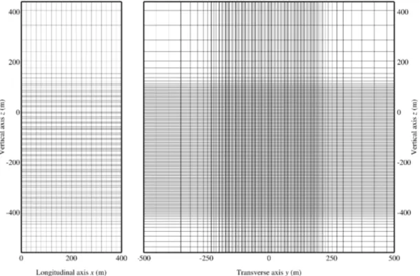
Figure 1.Vertical cross sections of the computational domain and along the contrail longitudinal axis (left panel) and transverse axis (right panel). The mesh is regular in the subdomain[0 m,400 m] × [−200 m,200 m] × [−350 m,+100 m]. For the sake of clarity, one out of five grid points are shown.
Figure 2.Vertical (left) and horizontal (right) cross sections of potential temperature differenceθ−θbin K for the atmospheric flow field
used in cases 2 and 4. The data from Paoli et al. (2014) are extracted in the regions delimited by the black boxes and used to initialize the present simulations.
the impact of this effect relative to other potential effects in Sect. 4.3. It is readily seen from Eq. (7) that the variation of crystal size depends on the local ice saturation ratio
s(xp)= ρv(xp)
ρv,ps,i
=Yv(xp) Yv,ps,i
≈pv(xp) psv,p,i
(11)
with respect to 1. Thus, the model can also deal with evapo-ration (dmp/dt <0) that occurs whens <1. The lower limit for crystal shrinking is the soot core diameterdn=20 nm.
3 Numerical setup and initial condition
Table 1.Reference values common to all cases. Aircraft data refer to a B747 (4-engines) aircraft. Exhaust jet values are expressed in meter of flight.
Quantity Unit Value(s)
Computational domain
Grid cells 100×519×619
Grid spacing1x×1y×1z m 4×1×1
DomainLx×Ly×Lz m 400×1000×1000
Atmosphere
Brunt–Väisälä frequencyN s−1 0.012
Reference altitudez0 m 11 000
Reference pressurep0 Pa 24 286
Wake vortices (B747 data)
Initial circulationŴ m2s−1 565
Core radiusrc m 4
Initial separationb m 47
Exhaust jets (B747 data)
Emitted vapor mass 4×Mv,e g m−1 4×3.75
Emitted nucleation sitesne m−1 1012
of wake vortex systems. The computational domain is a box of lengths Lx=400 m, Ly=1 km, and Lz=1 km in the
axial, transverse, and vertical directions, respectively. The axial domain is chosen to capture the long-wave instability of the vortex system (Crow instability). The reference trans-verse and vertical coordinates y0=0, z0=0 for the com-putational domain correspond to the position of the aircraft, which cruises at an altitude of 11 km. The mesh is regular with uniform grid spacing 1x=4 m in the axial direction and1y=1z=1 m in the region of the cross-sectional do-main containing the wake, while it is stretched far away from the wake (see Fig. 1). Periodic and open boundary conditions are imposed in the axial and transverse direction, respec-tively. In the vertical direction, all flow variables are relaxed toward a thermodynamic state representative of a stratified atmosphere with a uniform Brunt–Väisälä frequency (Paoli et al., 2013). The initial condition consists of an atmospheric flow field onto which the wake of the aircraft is inserted.
The background atmosphere is representative of an upper troposphere lower stratosphere region, i.e., stably stratified. The background thermodynamic variables Tb,pb andρb= pb/(RTb)depend onzand satisfy the relations
N2 g =
1 θb
dθb
dz, (12a)
dpb
dz = −ρbg, (12b)
Table 2.Table of simulations. The parameterǫis the eddy dissipa-tion rate of the background turbulence,η0is the relative turbulence
intensity,T0is the temperature at flight level, ands0is the
satura-tion ratio (in the whole domain). Across the following figures, each simulation is represented by a unique symbol or line pattern, which is indicated in this table.
Case ǫ( m2s−3) η0 T0(K) s0 Symbol and line
1 12.5×10⁻⁵ 0.095 218 1.30
2 1.6×10⁻⁵ 0.048 218 1.30
3 0.57×10⁻⁵ 0.034 218 1.30
4 1.6×10⁻⁵ 0.048 218 1.10
5 1.6×10⁻⁵ 0.048 218 0.95
6 1.6×10⁻⁵ 0.048 215 1.30
whereN=0.012 s−1is the Brunt–Väisälä frequency, while θbis the background potential temperature defined by
θb p(γθ −1)/γ
= Tb
pb(γ−1)/γ
, (13)
where pθ=105Pa and γ=1.4, the ratio of specific
heats for air. Pressure and density at flight level are kept fixed atpb(z0)=p0=242.86 hPa andρb(z0)=ρ0= 0.3881 m3s−1, while temperature at flight level, Tb(z0)= T0, is varied to analyze the effects of temperature on con-trail properties (see Table2). The background specific hu-midityYv,b is chosen to keep vapor saturation with respect to ice s0 constant in the computational domain: Yv,b(z)= s0Yvs,i(Tb(z)). Vapor saturations0 is also varied to analyze the effects of humidity on contrail properties. Atmospheric (or background) turbulence flow fields were provided by sep-arate LES of such stratified flows with specific eddy dissipa-tion rateǫ. Because of atmospheric stratification, turbulence is organized in horizontally layered structures, reflecting the anisotropy of turbulent fluctuations in the horizontal and ver-tical directions as shown in Fig. 2. In the work by Paoli et al. (2014), it was shown that a resolution of 4 m in the mid- and low-turbulence cases and 10 m in the strong-turbulence case are adequate to resolve the Ozmidov and buoyancy scales. Further details of the turbulent field are given in the Ap-pendix.
The initial turbulent fields for the present simulations were extracted from the larger computational domain as shown by the black box in Fig. 2. Periodic boundary conditions in the longitudinal direction are enforced by replacingf (Lx)=
f (0) for any variable f. Although this operation slightly modifies the background turbulent fields, the latter equili-brate to this constraint in a few time steps (furthermore, the amplitude of ambient fluctuations are small compared to the Lamb–Oseen vortex flow field).
J. Picot et al.: LES of contrails in atmospheric turbulence 7375
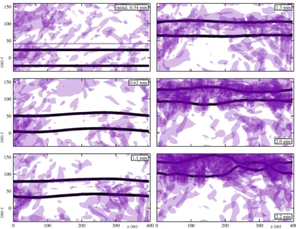
Figure 3.Top views of iso-contoursλ2=λ2,0/10 (black) andλ2=λ2,0/400 000 (colored) in a horizontal planexyat different instants
for case 2. Black contours show the cores of the trailing vortices, whereas the colored contours show the vortical structures of atmospheric turbulence. The development of instabilities is dominated by the long-wave (Crow) instability. The short-wave (elliptical) instability is also visible aftert=2 min as are secondary vorticity structures around each trailing vortex. The displacement of the wake along theydirection is due to the oscillation of a large-scale energetic mode in the background turbulent field.
Table 3.Summary of main contrail characteristics: lifespantb of
wake vortices, fraction of surviving crystals at the end of the vortex regime, and mean optical thicknessδ¯at the end of the vortex regime.
Case Lifespantb Fraction of surviving Optical thickness crystals at 4 min δ¯at 4 min
s % –
1 95 99.89 0.22
2 132 99.74 0.22
3 111 99.66 0.22
4 132 74.71 0.06
5 132 2.78 <0.03
6 118 99.71 0.18
of counter-rotating vortices and engine emissions including vapor and nucleation sites. Each vortex has a circulation of Ŵ=565 m2s−1 and a core radius rc=4 m, and the vor-tices are spaced by b=47 m. The mass of vapor emitted per unit flight distance isMv,e=3.75 g m−1per engine (the total emitted vapor is denoted byMv,0=15 g m−1) and the number of nucleation sites emitted per unit flight distance is
ne=1012m−1. Thus, the number of nucleation sites in the computational domain isn=4neLz, although the number of
numerical particles isnp=2×10⁶.
At this wake age all particles are already activated. In or-der to characterize the interaction between background tur-bulence and vortex dynamics, it is useful to introduce the relative turbulence intensityη0 that represents the velocity ratio between turbulent fluctuations and vortex descent ve-locity (Crow and Bate, 1976):
η0= vb w0=
2π Ŵ
3 p
ǫb4. (14)
The effective Reynolds number based on circulation Reeff=Ŵ/νtot, whereνtot=νmol+νsgs, ranges between 103 and 104 based on the maximum turbulent viscosity in the flow field and between 106and 107based on the mean turbu-lent viscosity.
in-tensity, respectively (this nomenclature is the same used by Paoli et al., 2014). Saturation has been reduced in cases 4 and 5 tos0=1.10 ands0=0.95, respectively. Finally, tempera-ture has been reduced in case 6 to T0=215 K. All simula-tions parameters are summarized in Tables 1 and 2.
4 Results
4.1 Dynamics of wake vortices
Wake vortices are detected using the λ2 field, which is defined as the second eigenvalue of the symmetric tensor S2+2 with S and being the symmetric and the anti-symmetric parts of the velocity gradient tensor, respectively (Jeong and Hussain, 1995). The vortex cores are charac-terized by negative values of λ2 with lower values corre-sponding to stronger vortices. The initial minimum value of λ2is found in the flow region inside the wake vortices, λ2,0=minx,y,z{λ2(x, y, z;0)} = −49.67 s−2, which is much smaller than the value corresponding to the vortex tubes of at-mospheric turbulence,λatm2 = −0.001 s−2. The evolution of λ2iso-surfaces reported in Fig. 3 illustrates the mechanism of vortex instability for the reference case. It is known from sta-bility analysis that counter-rotating vortices are prone to both long-wave (Crow) instability with wavelength λlw=8.6b and short-wave (elliptical) instability with wavelengthλsw= 0.37b (Crow, 1970; Widnall et al., 1970). For the present study, these values areλLW=405 m andλSW=17.4 m, re-spectively. The vortical structures identifying the wake vor-tices and the background turbulence are characterized by the values λ2=λ2,0/10 and λ2=λ2,0/400 000≈λatm2 /10, re-spectively. The figure shows that turbulence triggers pertur-bations of the wake vortex system that develop until the two vortex tubes collide and break up. The largest flow structure corresponds to the size of the axial domain and can then be identified withλLW. Starting att=2.0 min, the vortex tubes start to get closer and eventually collide att=2.2 min at two axial locations,x=250 m andx=350 m. In the other sim-ulations, a single collision between the vortex tubes is ob-served, see Fig. 4. It is also interesting to observe the emer-gence of another flow structure with wavelength of about 25 m starting at t=1 min, which can be identified with a short-wave instability. Although this has a higher growth rate (Widnall et al., 1970) than the long-wave instability, in the present case it is not sufficiently strong to overwhelm it and break the vortices before the latter develops. Elliptical instability in combination with Crow instability have been studied theoretically (e.g., Fabre et al., 2000), experimen-tally (e.g., Laporte and Leweke, 2000), and numerically (e.g., Paugam et al., 2010). Their emergence depends on character-istics of the vortex system (vortex core radius and spacing) and on the initial perturbation of the vortex system. Typi-cal perturbations include sinusoidal waves corresponding to the excited instability modes (Laporte and Corjon, 2000;
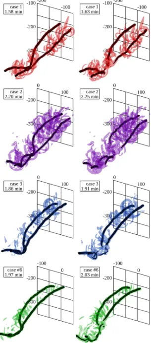
Le Dizès and Laporte, 2002; Paugam et al., 2010), broad-band white noise, and spectral perturbations satisfying model spectra of isotropic or anisotropic turbulence. The latter ap-proach has been used in the wake vortex literature and partic-ularly in the studies that attempted to analyze the interaction of the wake with the background turbulence (Lewellen and Lewellen, 1996; Gerz and Holzäpfel, 1999; Han et al., 2000; Holzäpfel et al., 2001) and more recently by Hennemann and Holzäpfel (2011) who focused on the identification of vortex flow topology, and by Misaka et al. (2012) who analyzed pas-sive scalar transport in addition to the fine-scale structures of the wake. The main difference with the present study is that here the background turbulence is sustained, yet the three-dimensional snapshots shown in these studies as well as the various pictures of wake instabilities reported in the literature Crow (1970), Chevalier (1973), and Sussmann and Gierens (1999) corroborate the structures visualized in Fig. 3. Isomet-ric views of iso-surfacesλ2=λ2,0/10 andλ2=λ2,0/1000 are drawn in Fig. 4 for cases 1, 2, 3, and 6 taken immedi-ately before and after the vortex tubes collide. The snapshots are similar for the three cases except for the double colli-sion appearing in case 2, which ensures the reproducibility of these flow structures by the present LES. In general, the vor-tex breakup always starts in the lowermost part of the wake because the wake descent is inversely proportional to the vor-tex separation (which goes to 0 at the collision point).
In order to measure the lifespan of wake vortices, their in-tensities are evaluated as a function of time: the minimum value ofλ2of each vortex is measured along the longitudi-nal axis. The conditionλ2< λ2,0/10 is used to discriminate
wake vortices from secondary vortices. Noticing on Fig. 4 that this condition may not be reached on some parts of the longitudinal axis, we define the vortex lengthxvas the length of the longitudinal axis range covering all axial sec-tions where this condition is verified. The length ratioxv/Lx
and the average vortex intensityλ¯2 are plotted in Fig. 5 for each vortex and for cases 1,2,3,and 6. The magnitude ofλ¯2 quickly decreases at the beginning before its rate of variation stabilizes at a constant value of−0.1|λ2,0|per minute. The ratioxv/Lxis initially equal to 1, meaning that coherent
J. Picot et al.: LES of contrails in atmospheric turbulence 7377
Figure 4.Iso-contoursλ2=λ2,0/10 (black) andλ2=λ2,0/1000
(colored) taken immediately before (left panels) and after (right panels) the vortex tubes collide. Black iso-contours represent the wake vortices, while colored iso-contours represent the secondary vortices.
All collected data show a similar trend: weaker relative tur-bulence leads to longer lifespan (as observed for example by Holzäpfel, 2003). Similar trends were recently reported us-ing the normalized Brunt–Väisälä frequencyN∗=N t0and the vortex sinking distancezb=w0×tbinstead of the vortex lifespan tb (Schumann, 2012; Jeßberger et al., 2013; Schu-mann et al., 2013), and Fig. 7 shows a general good agree-ment with those data.
0 1
xv
/
Lx
-1 ¯λ/2
|
λ2,
0
| case 1
left vortex (y<0)
right vortex (y>0)
0 1
xv
/
Lx
-1 ¯λ/2
|
λ2,
0
| case 2
left vortex (y<0)
right vortex (y>0)
0 1
xv
/
Lx
-1 ¯λ/2
|
λ2,
0
| case 3
left vortex (y<0) right vortex (y>0)
0 1
xv
/
Lx
-1
0 1 2 3 4
¯λ/2
|
λ2,
0
|
Wake aget(min)
case 6
left vortex (y<0) right vortex (y>0)
Figure 5.Time histories of vortex length ratiosxv/Lxandλ2/λ2,0.
for cases 1, 2, 3, and 6. The horizontal dashed lines for each case indicate the threshold valuesλ2=λ2,0/10 that is used to
discrim-inate the wake vortex tubes from the background turbulence. The two vertical dashed lines correspond to the times selected in the iso-contours of Fig. 4 (i.e., immediately before and after the vortex breakup) and define the lifespans of the wake vortices.
1 10
0.1
Lifespan
tb
/
t0
Turbulence intensityη0 Cessna 170
Boeing 727
Aero Commander 560 F
Figure 6.Lifespans of wake vortices as a function of relative tur-bulence intensity. The solid line is the analytical estimation by Crow and Bate (1976), the dashed line outlines lifespans obtained by numerical simulations of (Spalart and Wray, 1996), and black crosses are in situ measurements (Crow and Bate, 1976). Simula-tions:tions: casecase 1,
in-situ
1, case 2,2, casecase 3, andand casecase 6.
Figure 7.Non-dimensional maximum descentzb/bof wake vor-tices as a function of non-dimensional Brunt–Väisälä frequency N×t0for the present simulations and a collection of
experimen-tal and numerical data (adapted from Schumann (2012)).
Simula-tions:tions: casecase 1, in-situ
1, case 2,2, casecase 3, andand casecase 6. Note that
zb/b=w0×tb/b=tb/t0witht0=2π b02/ Ŵ. In all cases consid-ered in this study,t0≃25 s andN×t0≃0.3 (see Table1).
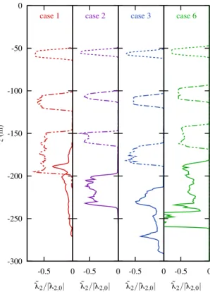
separation goes to 0, this phenomenon is observed again in Fig. 8 as the vertical spreading has accelerated att=2 min in cases 1, 3, and 6. Besides, the minimum value ofeλ2has in-creased towards 0 in cases 1 and 3 in accordance with Fig. 5. At the end of the vortex regime, the primary wake is found between 200 and 300 m below flight level.
-300 -250 -200 -150 -100 -50 0
-0.5 0
z
(m)
˜
λ 2/|λ2,0| case 1
-0.5 0 ˜
λ 2/|λ2,0| case 2
-0.5 0 ˜
λ 2/|λ2,0| case 3
-0.5 0 ˜
λ 2/|λ2,0| case 6
Figure 8.Vertical profiles ofeλ2/λ2,0that is used to track the wake
vortices as they move downwards and break up. The four pro-files shown for each case correspond toto t=0.5 min,, 655 t=1 minmin,, t=1.5 minmin,, tt=2 min.
4.2 Contrail microphysics
J. Picot et al.: LES of contrails in atmospheric turbulence 7379
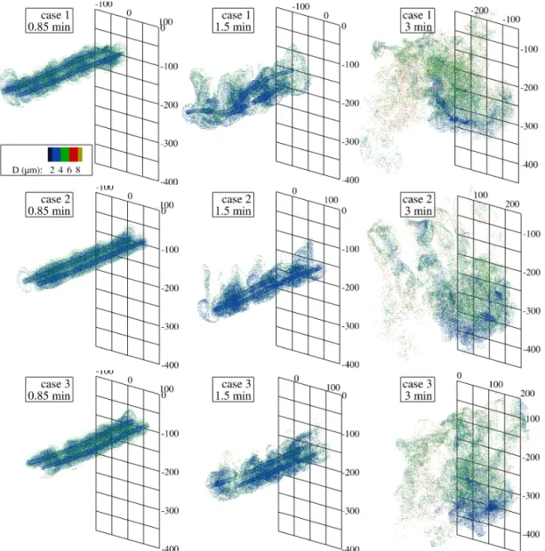
Figure 9.Snapshots of ice crystals spatial distribution for cases 1, 2, and 3. Crystals are colored with diameters. The figure shows the development of the secondary wake att=1.5 min and 3 min (center and right panels) and the formation of puffs att=3 min (right panels). It can be observed that the size of crystals slightly increases during the instability process of the vortex regime (t≤1.5 min), whereas it increases considerably in the dissipation regime (t=3 min) with larger crystals found in the secondary wake. Crystals appear more mixed in the strong atmospheric turbulence case (top panels).
and favors the development of Crow instability. The vertical extension reduces with the turbulence intensity because the vortices tend to destabilize and break up earlier in the case of strong turbulence compared to weak turbulence. This is further confirmed by the vertical profiles of ice crystal num-ber and mass reported in Fig. 10 taken at the same time as in Fig. 4.
Contrail diffusion is analyzed in Fig. 11 that shows the evolution of the contrail volume per unit flight distanceVp normalized by the initial volumeVp,0. The contrail volume is
computed as the sum of volume of the grid cells containing at least one crystal and defined over a regular mesh with 1 m of resolution. Up tot=1 min the volume expansion is
sim-ilar for the three turbulence levels. At approximatelyt=tb the volume expands faster with stronger turbulence, as also observed in snapshots of Fig. 9. It is interesting to note that the expansion rate is the same for all cases at the end of the simulation, even for case 6 (T0=215 K). This means that the wake turbulence is the main contributor to contrail dif-fusion in the dissipation regime (even though atmospheric turbulence is expected to become predominant as wake tur-bulence dissipates).
-300 -250 -200 -150 -100 -50 0
0 0.05
z
(m)
˜ n/np case 1
0 0.05
˜ n/np case 2
0 0.05
˜ n/np case 3
0 0.05
˜ n/np case 6
-300 -250 -200 -150 -100 -50 0
0 0.05
z
(m)
˜ Mi/Mv,0
case 1
0 0.05
˜ Mi/Mv,0
case 2
0 0.05
˜ Mi/Mv,0
case 3
0 0.05
˜ Mi/Mv,0
case 6
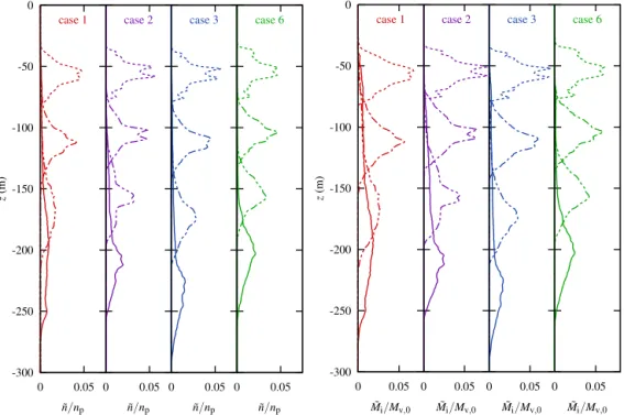
Figure 10.Vertical profiles of normalized numberen(z)/ntot (left panels) and massMei(z)/Mv,0 (right panels) of ice crystals. The four
profiles shown for each case correspond toto t=0.5 min,, 655t=1 min,min, t=1.5 min,min, tt=2 min.
0 100 200 300 400
0 1 2 3 4
Normalised
contrail
v
olume
Vp
/
Vp
,
0
Wake aget(min)
Vortex Dissipation
case 6 case 1 case 2 case 3 case 4 case 5
Figure 11. Normalized contrail volume per unit flight distance. Note the increased mixing following the vortex breakup where the exhaust material is released into the atmosphere.
Eq. (6): Mi= 1
Lz X
p
ncmp= 1 Lz
X
p ncπ
6d 3
pρice. (15) At the beginning of the vortex regime, the emitted water vaporMv,0has been completely deposed on ice crystals. The ambient vapor entrained in the plume during the first 10 s (see, e.g., Paoli et al., 2013) also contribute to the overall ice mass so that initially Mi> Mv,0. When ambient air is
sub-saturated (case 5), the ice mass decreases exponentially, con-sistently with observations of non-persistent contrails. When
0 1
2 3 4
5 6 7 8
0 1 2 3 4
Normalised
ice
mass
Mi
/
Mv
,
0
Wake aget(min)
Vortex Dissipation
case 1
case 2 case 3 case 4 case 5 case 6
Figure 12.Ice mass per unit flight distance normalized by the mass of emitted water vapor. Adiabatic compression reducesMi at the
end of the vortex regime, and this is particularly effective when the atmosphere is weakly supersaturated (case 4). The breakup of the vortices causesMito increase at a rate that depends on atmospheric
temperature, saturation, and, to a much lesser extent, turbulence.
J. Picot et al.: LES of contrails in atmospheric turbulence 7381
-400 -300 -200 -100 0
0 0.05
z
(m)
Mi/Mv,0 2.2 min 2.8 min 3.5 min 3.9 min 4.5 min
-500 -400 -300 -200 -100 0 100
0 0.01 0.02 0.03 0.04
z
(m)
˜ Mi/Mv,0
case 2
s0=1.3
0 0.01 0.02 0.03 0.04 ˜
Mi/Mv,0 case 4
s0=1.1
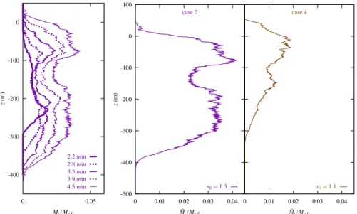
Figure 13.Vertical profiles of normalized massMei(z)/Mv,0. Left panel: profiles at different wakes ages in the dissipation regime for case
2. Right panel: comparison att=4.5 min between case 2 (s0=1.3) and case 4 (s0=1.1).
This decrease indicates the sublimation of crystals, explained by the process of adiabatic compression occurring in the pri-mary wake (Unterstrasser et al., 2008). However, the mix-ing of the secondary wake with ambient air partly compen-sates sublimation so that the ice mass reduction is less pro-nounced when increasing the turbulence intensity, and even completely compensates sublimation in case 1. In the dissi-pation regime, the ice mass grows again as the consequence of induced turbulence. Att=4 min,Mireaches 2Mv,0when s0=1.10 (case 4), 4.5Mv,0whenT0=215 K (case 6), and 8.5Mv,0whens0=1.30,T0=218 K, regardless of the tur-bulence level. The less-pronounced increase of ice mass for lower ambient temperature can be understood by observing that ambient saturation is kept constant between cases 2 and 6. Hence, the density of water vaporρv=sρvs,i(T )decreases when decreasing T (since ρvs,i is a monotonic function of temperature). In case 6, the mass of vapor entraining in the contrail and condensing into ice is then reduced compared to case 2 as shown in Fig. 12.
The vertical structure of the contrail is further analyzed in Fig. 13 in the dissipation regime. While the “curtain” con-necting the primary and secondary wakes forms as soon as the vortex pair start the descent, ice tends to substantially ac-cumulate in the secondary wake after the breakup until, at t=4.5 min, the two peaks are approximately the same for case 2 (s0=1.3). For case 4 (s0=1.1) most of ice crystals in the primary wake sublimated so that only the peak in the sec-ondary wake is apparent at the end of the dissipation regime. (Note these results closely resemble those obtained recently by Unterstrasser, 2014).
The number of particles surviving the adiabatic compres-sion is an important parameter to consider when evaluating
0 0.2 0.4 0.6 0.8 1
0 1 2 3 4
Ratio
of
acti
v
ated
particles
Wake aget(min)
case 1 case 2 case 3 case 4
case 5 case 6
Figure 14.Normalized number of activated particles (fraction of surviving crystals). Adiabatic compression is strong enough in weakly supersaturated atmosphere (case 4) to completely subli-mate 30 % of crystals, but it is not able to evaporate any crystals in strongly supersaturated atmosphere.
the global and climate impact of contrail (e.g., Burkhardt et al., 2010; Burkhardt and Kärcher, 2011).
0 0.2 0.4 0.6 0.8 1 1.2 1.4
0 1 2 3 4
Ratio
of
deposed
mass
Mi
/
Me
Wake aget(min) Vortex Dissipation
case 1 case 2 case 3
case 4
case 6
Figure 15.Ratio of deposed mass. In the vortex regime, the con-trail is close to equilibrium (Mi≈Me) only when the atmosphere is
strongly supersaturated. In the dissipation regime, the strong mix-ing between the contrail and ambient air causes a depart from the equilibrium state (Mi< Me).
It is interesting to evaluate the mass of ice that would be formed by a model that would enforce equilibrium between ice and vapor phase at each time step. This kind of models may be attractive as they are less computationally expensive. The equilibrium ice massMeis defined by
Me=Mi+Mv,awithMv,a= Z
Vp
ρv−ρvs,idVp (16)
and represents the ice mass of ice if all available vapor were instantaneously deposed onto crystals (note thatMv,ais not the available mass of vapor in the “true” situation). Figure 15 shows the ratio of deposed mass Mi/Me. At t=25 s, the ratio is close to 1 consistently with the equilibrium state suggested earlier in this section. The competition between ice sublimation due to the adiabatic compression and ice deposition by mixing of the secondary wake is seen again here at the end of the vortex regime. Turbulence favors mix-ing and entrainment of supersaturated ambient air into the plume. This in turn increases the ice deposition rate, which scales with the local supersaturation orYv(xp)(the amount of vapor available at particle position). When turbulence is strong (case 1) deposition is stronger than sublimation as Mi/Me.1, whereas when turbulence is weak (case 3) sub-limation is stronger than deposition asMi/Me&1. When su-persaturation is reduced to s0=1.10 (case 4), sublimation is much stronger than deposition and the equilibrium mass Meapproaches 0 (whileMi/Mediverges so the assumption of equilibrium is not valid fors0=1.10 ). In the dissipation regime, the ratioMi/Mereduces due to the mixing produced by the induced turbulence and reaches a constant value of 0.7 whens0=1.30 (regardless turbulence intensity or back-ground temperature) and 0.45 when s0=1.10. This result can be explained with an estimation of the rate of change of vapor in the contrail. On the one hand, the quantity of vapor
0.98
1 1.02
1.04 1.06
0 1 2 3 4
Mean
saturation
ratio
¯
s
Wake aget(min)
Vortex Dissipation
case 1 case 2
case 3
case 4
case 6
Figure 16.Mean saturation ratio computed as an ensemble average over all ice particles. The contrails is slightly subsaturated during the initial vortex descent between 1 and 2 min and supersaturated in the dissipation phase after 2 min.
is increased by mixing at a rate ofQm=s0ρvs,i(T0)dVp/dt, neglecting temperature variations in the contrail vicinity. On the other hand, the quantity of vapor is decreased by deposi-tion at a rate ofQd=ndmp/dt=Cn(s−1)ρsv,i(T0), where Cdepends on the mean particles radius and can be assumed constant between 1 and 2 min as the ice mass (see Fig. 12). The temperature dependence ofG(Knp)Dv,p in Eq. (7) can reasonably be neglected in this context. Figure 15 shows that theses rates are balanced at the end of the simulation. WhenT0is reduced, bothQmandQdare decreased by the same amount, which does not change the balance (although the time needed to reach this balance increases). When s0 is reduced by 15 % from 1.30 to 1.10, Qm is reduced by 15 % whileQdis reduced (throughn) by 25 %, and the bal-ance is then changed towards higher amounts of vapor in the contrail. A potential drawback in the definition of Mv,a in Eq. (16) is that it depends on the definition of Vp, which may not be suitable to evaluate the non-equilibrium in the actual contrail. To that end, we calculated the mean satura-tion ratiosby means of an ensemble averages(xp)over all ice particles. Its evolution is shown in Fig. 16. In the mid-dle of the vortex phase between 1 and 2 min, thermodynamic conditions are very close to equilibrium (relative humidity is slightly less than 100 %) because of the sublimation due to adiabatic heating balancing the deposition due to the en-trainment of fresh ambient vapor (similar levels of relative humidity were observed for example by Naiman et al., 2011, their Fig. 8). In the dissipation phase humidity is greater than 100 % as the ice crystals originally trapped in the vortices are fully exposed to ambient vapor although it does not exceed 105 % for the conditions of this study.
The optical thickness of the contrailδ¯is shown in Fig. 17. It is evaluated by first computing the optical thicknessδ(Sxy)
over each columnSxy= [x, x+1x[×[y, y+1y[×Lz and
J. Picot et al.: LES of contrails in atmospheric turbulence 7383
0
0.1
0.2 0.3 0.4
0 1 2 3 4
Mean
optical
thickness
¯δ
Wake aget(min)
Vortex Dissipation
case 1 case 2
case 3 case 4
case 5
case 6
! △ ♦
△
♦
Figure 17.Mean optical thickness. The horizontal black line rep-resent the visibility criterion δ >¯ 0.03 (Kärcher et al., 1996). The mean optical thickness decreases during the vortex regime and sta-bilizes during the dissipation regime. Its evolution depends mainly on atmospheric temperature, saturation, and, to a lesser extent, tur-bulence. The symbols on the right of the figure shows the values of the optical thickness for different aircraft and atmospheric situa-tions measured in the CONCERT campaign (Voigt et al., 2011) as reported by Jeßberger et al. (2013).
is assimilated to a monochromatic wave of wavelengthλ0= 550 nm, the refractive index of water isµ0=1.31, and the extinction coefficient Qis approximated by the anomalous diffraction theory (Van De Hulst, 1957):
Q(ρ)=2−4 ρsinρ+
4
ρ2(1−cosρ), (17)
whereρ≡2π(µ0−1)dp/λ0. Over a columnSxy, the optical
thickness is computed as follows δ(Sxy)=
1 1x1y
X
xp∈Sxy
ncπ 4d
2
pQ(ρ). (18)
In Fig. 17, when ambient air is not saturated (case 5), δ¯ decreases exponentially and, by 2.5 min, it falls below the thresholdδ <¯ 0.03 used by Kärcher et al. (1996) as a visi-bility criterion. Although the visivisi-bility of a contrail does de-pend not only on the optical depth but on many other param-eters (angle between observation and sun, contrast against background, aerosols between observer and contrail, etc.), the simplistic treatment used here is in line with those em-ployed in previous numerical simulations of contrails (Un-terstrasser and Gierens, 2010a; Naiman et al., 2011). When ambient air is supersaturated, δ¯ increases by 25 % of the initial value by the time the contrail reaches the equilib-rium state. Afterwards,δ¯decreases by the end of the vortex regime, which is due to the microphysical processes men-tioned above combined with the dilution of the contrail that reduces the number density of ice crystals and thusδ¯in ev-ery cases. In case 4 (s0=1.10), the more pronounced sub-limation results in a stronger reduction of δ. In the early¯
stages of the dissipation regime, the mean optical thickness has larger fluctuations that are possibly due to the induced wake turbulence and to the form of the extinction coefficient that is an oscillating function of the argument (in particu-lar the ice crystal diameterdp). As the contrail expands and diffuses, these oscillations are damped and the optical thick-ness attains a value of around 0.06 whens0=1.10 (case 4), 0.18 when T0=215 K (case 6), and 0.22 whens0=1.30, T0=218 K, regardless of the turbulence level. Mean contrail optical thickness of the order of 0.2 to 0.3 were reported by Voigt et al. (2011) and Jeßberger et al. (2013) for the CON-CERT campaign and similar aircraft. Jeßberger et al. (2013) also reported qualitatively similar results with the EULAG-LCM LES model (Sölch and Kärcher, 2010) and the CoCiP model (Schumann, 2012), i.e., 0.05<δ <¯ 0.1 in weakly su-persaturated atmospheres and 0.1<δ <¯ 1 in strongly super-saturated atmospheres. Optical thickness is lower whens0or T0is reduced as they both reduce density of water in the at-mosphere.
100
101
102
103
104
d
n
/
d
ln
dp
(cm
−
3)
case 2 5 s
1 min 3 min
100
101
102 103 104
d
N
/
d
log
D
(cm
−
3)
case 4 5 s
1 min 3 min
100
101
102 103 104
d
N
/
d
log
D
(cm
−
3)
case 5 5 s
1 min 3 min
Figure 18. Crystal diameter distributions at 5 s, 1 min, 3 min for the three levels of saturation and measurements from Schröder et al. (2000) (bottom).
due to the limited number of numerical particles and should lead to an underestimation ofδ. However, the coefficients of¯ the summation in Eq. (18) scale withdp2, which mitigates the effect of missing the smallest particles on the mean optical thickness. Despite these differences, Fig. 18 shows a reason-able agreement in terms of order of magnitude and shape of the crystal diameter distribution.
0 0.2 0.4 0.6 0.8 1
ni
/
np
case 2 case 2 + Kelvin
case 4 case 4 + Kelvin
0
0.1 0.2 0.3
0 1 2 3 4
¯δ
Wake aget(min)
Vortex Dissipation
Figure 19.Top panel: normalized number of activated particles (fraction of surviving crystals). Bottom panel: mean optical thick-ness. Plain lines indicates simulations with the Kelvin effect acti-vated.
J. Picot et al.: LES of contrails in atmospheric turbulence 7385 5 Discussion and conclusions
This study presented the results of three-dimensional large-eddy simulations of contrail evolution in the vortex and dis-sipation regimes of an aircraft wake immersed in a turbulent atmospheric flow field. The computational model is based on an Eulerian–Lagrangian two-phase flow formulation where clusters of ice crystals are tracked as they move in the wake. The background turbulence and the initial condition for the contrail at the end of the jet regime were both generated from appropriate simulations. The focus of the study is to evaluate the effects of atmospheric turbulence on the wake dynamics and the contrail properties and to compare with the effects of ambient humidity and temperature. The results showed a good agreement with numerical and experimental literature work, in terms of descent and lifespan of wake vortices, over-all mass of ice produced, and optical depth. Visual patterns of the primary and secondary wakes, Crow instability, and the formation of “puffs” also resembled qualitatively those found in observational analysis. The agreement of particle diameter distribution was also acceptable given the large data scatter and uncertainty of both ambient conditions and soot particle emissions in the experimental campaigns compared to those considered in the present study.
The main effect of atmospheric turbulence in the vortex regime is to trigger instabilities in the wake vortices and to accelerate their descent. Stronger turbulence accelerates the onset of the instability, leading to shorter contrail descent and more effective mixing in the interior of the plume. These re-sults are in line with those published in recent wake vortex literature (Holzäpfel et al., 2001; Hennemann and Holzäpfel, 2011; Misaka et al., 2012) – although the latter authors ana-lyzed weaker turbulence scenarios than ours – and are then a solid basis to investigate their impact on contrail micro-physics. These effects influence the lifetime of the vortices, the vertical extent of the contrail, and the number of sur-viving crystals. Atmospheric turbulence is then an impor-tant driver of the contrail evolution in the vortex and dis-sipation regime, which cannot be captured when the vortex instability is triggered by explicitly forcing one or more spe-cific modes of the vortex system (Paugam et al., 2010). How-ever, it is found that the self-induced turbulence that is pro-duced in the wake after the vortex breakup dominates over the background turbulence and effectively controls the mix-ing of the wake with ambient air. As a result, the intensity of the latter has a small impact on the microphysical and opti-cal properties at timesopti-cales of 4 min after emission. Contrail microphysics is strongly influenced by atmospheric tempera-ture and saturation, which control the mass of water vapor in contrail surroundings, and the number of surviving crystals. In addition, the mixing induced by the wake turbulence gen-erated during the vortex breakup in the dissipation regime is able to break the equilibrium between water vapor and ice phases inside the contrail, reducing the mass of ice by more than 30 % compared to model that would enforce
equi-librium. Note that once the wake turbulence has decayed, one can expect that background turbulence would be again the main driver of contrail dynamics in the early diffusion regime. This is the object of current investigation.
The mean contrail properties are in line with recent re-sults obtained by numerical simulations that explored a larger set of parameter space (Lewellen et al., 2014; Unterstrasser, 2014). However, for the high supersaturated cases,s0=1.3, the present study consistently shows a reduced crystal loss with more than 99 % crystals surviving, whereas, for exam-ple, Unterstrasser (2014) predicts that 90 % crystals survive ats0=1.4. As pointed out by Lewellen et al. (2014) and con-firmed by Unterstrasser (2014), the onset of crystal loss is de-layed and the crystal loss is increased when the Kelvin effect in the ice growth rate is switched off. We did observe these phenomena when comparing the same situations without and with Kelvin effect activated although its impact was in gen-eral lesser than what was found by Lewellen et al. (2014). Another factor that can potentially impact the prediction of crystal loss is the treatment of vapor mixing. Indeed, the de-position rate, Eq. (7), depends on the local vapor field which is sensitive to the numerical scheme adopted for scalar ad-vection (Unterstrasser et al., 2014), especially in the zones of high gradients as those occurring in the dissipation regime where the exhausts trapped in the wake is released and mix efficiently with ambient air. Whether it is the microphysical setup or the scalar advection schemes (e.g., high-order vs. low-order numerical schemes, upwind vs. centered schemes) that is mainly responsible for the difference in the deposition rate and the crystal loss in this phase is a point that deserves further investigation in follow-up studies.
Appendix A: Details of the atmospheric turbulence field In the large domain used to generate the ambient turbu-lence (Lbox=4 km,1=4 m) the root mean squares (rms) of horizontal velocity fluctuations wereσu≃σv≃0.4 m s−1, while the anisotropy ratio between the rms of horizontal and vertical fluctuations was σu/σw≃4 (see Table 1 in Paoli et al., 2014). The integral length scale (estimated as Lt=
3π
4K Z ∞
0 E(k)
k dk, withK=1/2(σ 2
u+σv2+σw2)as the turbulent kinetic energy, kthe horizontal wave number, andE(k)the kinetic energy horizontal spectrum) ranged between 700 and 1 km. Because the ratioLt/b≫1, the integral length scale
does not significantly affect the vortex decay as observed in previous studies (e.g., Crow and Bate, 1976; Hennemann and Holzäpfel, 2011). When the atmospheric turbulent flow field is truncated within the smaller domain denoted by the black box in Fig. 1, it will adapt to the new boundary conditions with a timescale that can be estimated asτ=σu2vor/ǫ, where σu2vor is the rms velocity calculated in the regular portion of the contrail domain (and similar expression for the ver-tical direction). We reported these values in Table A1, which shows that in all casesτ >5 min. Hence, we can reasonably assume that ambient turbulence remains frozen (and the con-ditionLt/b≫1 remains valid) during the vortex phase.
A1 Details of sgs turbulent viscosity
The subgrid-scale model in this study is based on filtered structure function by Ducros et al. (1996) that provides at each grid node the turbulent viscosity reconstructed locally using the nine closest grid points surrounding the grid node. Figure A1 shows the evolution of the minimum (νsgsmin), max-imum (νsgsmax), and mean (νsgsmean) values of turbulent vis-cosity in the field, normalized by the molecular visvis-cosity νmol. The ratioνsgsmean/νmol∼10 at the breakup time (where the gradients are the largest), which is an a posteriori con-firmation of the good performance of the sgs model and the resolution employed here. Peak values of this ratio are of course larger although they are local in nature as they correspond to specific points in the flow field. We com-puted the effective Reynolds numbers based on the circu-lationReeff(νsgs)=Ŵ/νtotwithνtot=νmol+νsgs, which are also reported in Fig. A1 for the corresponding minimum, maximum, and mean values of turbulent viscosity. The val-ues based on the maximum turbulent viscosity (worst situa-tion) areReeff(νsgsmax)∼104except for a short interval at the breakup time and in line with previous LES of the vortex phase (e.g., Gerz and Holzäpfel, 1999).
Table A1.Horizontal and vertical rms velocities measured in the regular subdomain.
η0 σuvor(m s−1) σwvor(m s−1) τ (min)
0.095 (case 1) 0.41 0.15 47
0.048 (cases 2, 4, 5, 6) 0.23 0.08 15
0.095 (case 3) 0.17 0.05 8
103 104 105 106 107
Re
ef
f
,
Re
mol
Reeff(νsgsmean)
Reeff(νmax
sgs )
Reeff(νmin
sgs) Remol
10−3 10−2 10−1 100 101 102 103 104
0 1 2 3 4
νsgs
/
νmol
Wake aget(min)
Vortex Dissipation
νmax
sgs
νsgsmean
νmin
sgs
Figure A1.Top panel: evolution of the turbulent-to-molecular vis-cosity ratio. The three curves correspond to the minimum (νsgsmin), maximum (νsgsmax), and mean (νsgsmean) values of turbulent viscosity. Bottom panel: evolution of the effective Reynolds numbers based on circulation and total viscosity:Reeff=Ŵ/νtotwithνtot=νmol+
νsgsfor the corresponding values of turbulent viscosity shown in the
J. Picot et al.: LES of contrails in atmospheric turbulence 7387
Acknowledgements. Financial support from the Direction Général
de l’Aviation Civile through the project TC2 (Traînés de Con-densation et Climat) is gratefully acknowledged. Computational resources were provided by CINES supercomputing center. The authors wish to thank the two referees for their constructive comments that helped to improve the paper.
Edited by: C. Voigt
References
Barone, M. F.: Receptivity of compressible mixing layers, PhD the-sis, Stanford University, 2003.
Boivin, M., Simonin, O., and Squires, K. D.: Direct nu-merical simulation of turbulence modulation by particles in isotropic turbulence, J. Fluid Mech., 375, 235–263, doi:10.1017/S0022112098002821, 1998.
Brethouwer, G., Billant, P., Lindborg, E., and Chomaz, J.-M.: Scal-ing analysis and simulation of strongly stratified turbulent flows, J. Fluid Mech., 585, 343, doi:10.1017/S0022112007006854, 2007.
Burkhardt, U. and Kärcher, B.: Global radiative forc-ing from contrail cirrus, Nat. Clim. Chang., 1, 54–58, doi:10.1038/nclimate1068, 2011.
Burkhardt, U., Kärcher, B., and Schumann, U.: Global Modeling of the Contrail and Contrail Cirrus Climate Impact, B. Am. Meteo-rol. Soc., 91, 479–484, doi:10.1175/2009BAMS2656.1, 2010. Chevalier, H.: Flight Test Studies of the Formation and Dissipation
of Trailing Vortices, Tech. Rep. 730295, SAE International, War-rendale, PA, 1973.
Crow, S. C.: Stability Theory for a Pair of Trailing Vortices, AIAA Journal, 8, 2172–2179, doi:10.2514/3.6083, 1970.
Crow, S. C. and Bate, E. R., J.: Lifespan of trailing vor-tices in a turbulent atmosphere, J. Aircraft, 13, 476–482, doi:10.2514/3.44537, 1976.
Ducros, F., Comte, P., and Lesieur, M.: Large-eddy simula-tion of transisimula-tion to turbulence in a boundary layer devel-oping spatially over a flat plate, J. Fluid Mech., 326, 1–36, doi:10.1017/S0022112096008221, 1996.
Fabre, D., Cossu, C., and Jacquin, L.: Spatio-temporal development of the long and short-wave vortex-pair instabilities, Phys. Fluids, 12, 1247–1250, doi:10.1063/1.870375, 2000.
Gamet, L., Ducros, F., Nicoud, F., and Poinsot, T. J.: Com-pact finite difference schemes on non-uniform meshes. Appli-cation to direct numerical simulations of compressible flows, Int. J. Numer. Meth. Fl., 29, 159–191, doi:10.1002/(SICI)1097-0363(19990130)29:2<159::AID-FLD781>3.0.CO;2-9, 1999. Gerz, T. and Ehret, T.: Wingtip vortices and exhaust jets during the
jet regime of aircraft wakes, Aerosp. Sci. Technol., 1, 463–474, doi:10.1016/S1270-9638(97)90008-0, 1997.
Gerz, T. and Holzäpfel, F.: Wing-Tip Vortices, Turbulence, and the Distribution of Emissions, AIAA Journal, 37, 1270–1276, doi:10.2514/2.595, 1999.
Gerz, T., Dürbeck, T., and Konopka, P.: Transport and effective diffusion of aircraft emissions, J. Geophys. Res., 103, 25905– 25913, doi:10.1029/98JD02282, 1998.
Gerz, T., Holzäpfel, F., and Darracq, D.: Commercial aircraft wake vortices, Prog. Aerosp. Sci., 38, 181–208, doi:10.1016/S0376-0421(02)00004-0, 2002.
Han, J., Lin, Y.-L., Schowalter, D. G., Pal Arya, S., and Proctor, F. H.: Large Eddy Simulation of Aircraft Wake Vortices Within Homogeneous Turbulence: Crow Instability, AIAA Journal, 38, 292–300, doi:10.2514/2.956, 2000.
Hennemann, I. and Holzäpfel, F.: Large-eddy simulations of air-craft wake vortex deformation and toplogy, J. Aerospace Eng., 25, 1336–1350, doi:10.1177/0954410011402257, 2011. Holzäpfel, F.: Probabilistic two-phase wake vortex decay and
trans-port model, J. Aircraft, 40, 323–331, doi:10.2514/2.3096, 2003. Holzäpfel, F., Gerz, T., and Baumann, R.: The turbulent decay of
trailing vortex pairs in stably stratified environments, Aerosp. Sci. Technol., 5, 95–108, doi:10.1016/S1270-9638(00)01090-7, 2001.
Holzäpfel, F., Hofbauer, T., Darracq, D., Moet, H., Garnier, F., and Gago, C. F.: Analysis of wake vortex decay mecha-nisms in the atmosphere, Aerosp. Sci. Technol., 7, 263–275, doi:10.1016/S1270-9638(03)00026-9, 2003.
Huebsch, W. W. and Lewellen, D. C.: Sensitivity studies on con-trail evolution, in: 36th AIAA Fluid Dynamics Conference and Exhibit, San Fransisco, California, doi:10.2514/MFDC06, 2006. Jeong, J. and Hussain, F.: On the identification of a vortex, J. Fluid
Mech., 285, 69–94, doi:10.1017/s0022112095000462, 1995. Jeßberger, P., Voigt, C., Schumann, U., Sölch, I., Schlager, H.,
Kauf-mann, S., Petzold, A., Schäuble, D., and Gayet, J.-F.: Aircraft type influence on contrail properties, Atmos. Chem. Phys., 13, 11965–11984, doi:10.5194/acp-13-11965-2013, 2013.
Kärcher, B. and Yu, F.: Role of aircraft soot emissions in contrail formation, Geophys. Res. Lett., 36, L01804, doi:10.1029/2008GL036649, 2009.
Kärcher, B., Peter, T., Biermann, U. M., and Schumann, U.: The Initial Composition of Jet Condensation Trails,
J. Atmos. Sci., 53, 3066–3083,
doi:10.1175/1520-0469(1996)053<3066:TICOJC>2.0.CO;2, 1996.
Kärcher, B., Busen, R., Petzold, A., Schröder, F. P., Schumann, U., and Jensen, E. J.: Physicochemistry of aircraft-generated liquid aerosols, soot, and ice particles 2. Comparison with observations and sensitivity studies, J. Geophys. Res.-Atmos., 103, 17,129– 17,147, doi:10.1029/98JD01045, 1998.
Laporte, F. and Corjon, A.: Direct numerical simulations of the el-liptic instability of a vortex pair, Phys. Fluids, 12, 1016–1031, doi:10.1063/1.870357, 2000.
Laporte, F. and Leweke, T.: Elliptic Instability of Counter-Rotating Vortices: Experiment and Direct Numerical Simulation, AIAA J., 40, 2483–2494, doi:10.2514/2.1592, 2000.
Le Dizès, S. and Laporte, F.: Theoretical predictions for the ellipti-cal instability in a two-vortex flow, J. Fluid Mech., 471, 169–201, doi:10.1017/S0022112002002185, 2002.
Lee, D. S., Fahey, D., Forster, P., Newton, P., Wit, R., Lim, L., Owen, B., and Sausen, R.: Aviation and global climate change in the 21st century, Atmos. Environ., 43, 3520–3537, doi:10.1016/j.atmosenv.2009.04.024, 2009.
Lele, S. K.: Compact finite difference schemes with spectral-like resolution, J. Comput. Phys., 103, 16–42, doi:10.1016/0021-9991(92)90324-R, 1992.