Abstract—This paper presents a novel approach to predict Taiwan pollution consumptions based on grey theory models (GM). In this research, we propose the four grey models for the prediction of Taiwan pollution consumptions (pollution gas: CO2; CH4; N2O; HFCS; PFCS; and SF6). The first and N-order with single variable (GM (1, 1)) model and multiple variables (GM (1, N)) model are applied in domestic pollution system that was developed and tested on their performances. Based on these models GM (1, 1); RGM (1, 1); GM (1, N) and RGM (1, N) are predicted and compared with those of the manufacturing environment data in Taiwan’s industry manufacturers (Energy; Manufacturing; Transportation; Agricultural; Service; Housing; and Production Industry). Simulation results show that the prediction accuracy of models GM (1, N) & RGM (1, N) presented the better accuracy than models GM (1, 1) & RGM (1, 1). This research is successfully applied these design models for producing more accuracy information for pollution controllers.
Key words: Forecasting, Grey theory, Pollution Management
I. INTRODUCTION
NDUSTRIAL pollution management is a difficult challenge to the manufacturers of world-wide supply chains. Many manufacturers are incapable to achieve the requirements of environmental regulations from WEEE and RoHS management [15]. One of major reasons is the lack of pollution management experiences and an effective predicting system for improving uncertainty management. Many pollution controllers attempted to predict pollution situations for industrial environment by different forecasting algorithms. They attempted to apply the causal method, the linear regression model, time series model [7], and Markov method that are successfully designed for the applications in different industrial fields with sufficient samples [11].
Nevertheless, in real market, the lead-time is short and the applicable data is limited [14]. This situation will increase the difficult of prediction management and reduce the precision levels of forecasting models [2],[3]. Many studies have discovered that grey theory models can overcome these weaknesses. In recent years, various prediction models of grey theory have verified that these proposed models can significantly improve the accuracy of limited data forecasts. Several researchers have also applied grey prediction models in manufacturing industries to lower inventory levels for minimizing their green costs [1],[10].
Manuscript received March 7, 2012; revised March 29, 2012. Chen-Fang Tsai is with the Department of Industrial Management and Enterprise Information, Aletheia University, Taipei, Taiwan. (Corresponding author phone: +886226212121~6113; fax: +886224931268; e-mail: [email protected] ).
Green management is not only to apply in recycle materials, but also to minimize pollution consumptions in manufacturing industries [6],[10]. The environmental pollutions are contained by various interacting factors that effected and determined the pollution gas levels [9],[13] (such as: CO2;
CH4; N2O; HFCS; PFCS; and SF6). We attempt to apply the
pollution consumption output of industrial supply chains in Taiwan from 2001 to 2009 as an example for verifications. Three grey prediction models, RGM(1,1); GM(1,N) and RGM(1,N), are chosen for the purpose of comparison with GM(1,1) by their prediction accuracy.
To assess the effectiveness and efficiency of this prediction design, the several comparisons were conducted by depending the prediction complexities of industrial affecting factors. The results show that models GM(1,N) & RGM(1,N) are more accurate than the other two models GM(1,1) & RGM(1,1) in both waste air and manufacturing industry predictions. This approach can significantly improve the accuracy of limited data forecasts. The paper is organized as follows. Section II provides literature review. Section III proposes the prediction behaviors and architecture of grey theory. Section IV presents grey models and their design procedures. Section V Experimental Results. Finally we draw some general conclusions. The next section initiates to portray the literature review in different prediction algorithms and grey theory.
II. LITERATURE REVIEW
Various prediction algorithms have been developed over the decades, including the causal method, the linear regression model, time series model, Markov methods, etc. [11] and designed in different fields. The causal method needs an enough historical data to analyze the relations in their variables. The linear regression method assumes that related factors are independent with normal distribution in forecasting processes. The time series model needs the stable tendencies in the prediction situations [4]. The Markov model requires recognizing the alteration probability among every state of the prediction process [11].
In practical industries, these approaches are complicated to gather sufficient samples to satisfy their constraints. The researcher frequently faced uncertain circumstances with partial data and vague information for their predicting researches. Hung [8] designed a GA based GM(1,1) mode to predict the short lead-time. Several studies proposed the GA based GM(1,1) mode for short-term data prediction [6]. Similar researches designed the rolling grey prediction algorithm and the transformed grey prediction methodologies that can improve the GM(1,1) mode by adjusting prediction strategies. There are numerous obstacles: (1) generating the coefficient value (X) by a constant value of 1/X probably may not achieve the optimal forecast accuracy; (2) when the
The Application of Grey Theory to Taiwan
Pollution Prediction
Chen-Fang Tsai
contiguous data are the same, it is difficult to achieve the better forecasting model; (3) The too old data cannot disclose latest situations and may produce a decline forecasting accuracy [2] [3].
Grey procedures are included by the grey generation; the grey relational analysis; the grey model; the grey forecasting in GM(1,1); and GM (1,N) models for these forecasting approaches [9]. Grey forecasting model, GM(1,1): start with original data and set-up the background data procedure and then, generate accumulated data (Accumulated Generating Operation AGO). The prediction equations are produced by least squares method for solving then, substitute the estimate parameter value into the time period series of differential equations. Subsequently, the IAGO (Inverse Accumulated Generating Operation IAGO) will be obtained by deduction procedure to generate the type of an inverse accumulative deduction regressive series. It can be obtained the prediction model after deduction processing.
This study designed the prediction models of grey theory for Taiwan pollution consumptions [13] and also defined the grey relations of pollution factors in these management models [7] [12]. The aim of this article is to construct a forecasting model based on grey theory by the limited information of pollution management. Unlike statistical methods, this theory mainly deals with original data by accumulated generating operations (AGO) and tries to find its internal regularity. Deng [11] has been proven that the original data must be taken in consecutive time period and as few as four data. In addition, the GM (1,N)model is the core of grey system theory and the GM (1,1) is one of the most traditional grey models.
III. THE PREDICTION BEHAVIORS AND ARCHITECTURE OF GREY THEORY
The experimental model contains four steps as follows: Firstly, the experiment of (GM (1,1) & RGM (1,1)) models. Secondly, the relation analysis of GM (1,N) model. Third, the prediction simulation of ((GM (1,N) & RGM (1,N)). Fourth, The comparisons of grey series ((GM (1,1); RGM (1,1); GM (1,N); and (RGM (1,N)). (see Figure. 1).
Figure. 1 The comparisons of grey model series
The following steps explain the GM(1,1) model: (1). Collect and define the original data (Xi(0)(t)). (2). Establish the
accumulated data (Xi(1)(t)) (AGO). (3). Set-up the background
model procedure. (4). Establish the differential equation procedure. (5). Establish the whitening equation. (6). Find the coefficient (a) & input value (b). (7). Establish the final value of whitening equation. (8). Establish the inverse AGO value
(IAGO) for the prediction data (Ã(I=0)(t)). (9). The final
procedure is the residual test that GM(1,1) model respectively the original data (Xi(0)(t)) and the prediction data (Ã(I=0)(t)) for
the modified residual model RGM(1,1).
The grey relation analysis of GM(1,N) model explained as following three steps: (1). calculate the average of the original sequence, and then divide by the corresponding sequence using the mean of each data, new data can be obtained. (2). grey relational analysis is calculated in the grey relational space. There is a reference series in this sequence reference; others are the compare series in these columns. (3). Grey correlation is calculated by the final size of the correlation of grey correlation in accordance with the size of sorting the results, higher correlation that the higher the degree [7] [12].
IV. GREY MODELS AND PROCEDURES DESIGN There are the 11 procedures of ((GM (1,1); RGM (1,1); GM (1,N); and (RGM (1,N)) models that are discussed as follows: GM (1,1):
Procedure 1: Collect the original data.
(1), (2), , ()
) , , 2 , 1 ) (
( (0) (0) (0) (0)
) 0
(
tt n
n
(Equation 1)Procedure 2: Establish the accumulated data (AGO).
(1)(
1
),
(1)(
2
),...,
(1)(
)
) 1
(
n
1 1 1 ) 0 ( 2 1 ) 0 ( ) 0 ((
),
(
),
,
(
)
t n t tt
t
t
(Equation 2)Procedure 3: Set-up the background model.
)
1
(
5
.
0
)
(
5
.
0
)
(
(1) (1)) 1 (
0
t
t
t
z
(Equation 3)Procedure 4: Establish the differential equation.
b
t
a
dt
t
d
(
)
)
(
(1) ) 1 (
(Equation 4) Procedure 5: Establish the whitening equation.b
t
az
t
)
(
)
(
(1) )0 (
(Equation 5) Procedure 6: Find the coefficient (a) & input value (b).
b
a
Y
B
B
B
T 1 T nˆ
(Equation 6) Procedure 7: Establish the final value of whitening equation.a
b
e
a
b
t
at
1
)
(
(
1
)
)
(
ˆ
(1)
(0)
(Equation 7)Procedure 8: Establish the inverse AGO value (IAGO). ) 1 ( ) 0 ( ) 0
(
(
)
(
1
)
(
1
)
ˆ
a ate
a
b
e
t
(Equation 8)RGM (1,1):
Procedure 9: Residual Test ofGM (1,1). (1). Residual series
(0)(
t
)
-
ˆ
(0)(
t
)
:)
(
ˆ
)
(
)
(
(0) (0) )0
(
t
t
t
(Equation 9)(2). Residual series
(0)(
t
)
by GM(1,1) model:
e t n
a b e
t t
t a at
, , 3 , 2 , ) 1 ( ) 1 ( 1 , ) ( ) (
ˆ (0) ( 1)
) 0 ( ) 0 (
(Equation 10)
(3). Substitution
(0)(
t
)
&
ˆ
(0)(
t
)
: The comparisons of ((GM (1,1);RGM (1,1); GM (1,N); (RGM (1,N))The experiments & relation analysis of grey factors
The experiment of GM (1,1)
The residual test of RGM (1,1) The residual test of RGM (1,N)
% 100 ) ( ) ( ˆ ) ( )
( (0)
) 0 ( ) 0 ( t t t t e
(Equation 11)
Apply the residual values of GM(1,1) mode to re-operate the Procedure 1 to 8 of GM(1,1).
GM (1,N):
Procedure 10: The grey relation analysis of original series (
0) and references series (
i) [7],[12].. max ) ( . max . min )) ( ), ( ( 0 0 t t t i
i (Equation 12)
( 0
(
t
)
0(
t
)
(
t
)
i
i
; by (
0(
t
)
) &(
i(
t
)
);
0
,
1
(distinguishing coefficient)).)
(
min
min
min
0it
t
i
;
max
max
max
0i(
t
)
t i
.The equation of average grey relations:
nt
i
i
t
t
n
1 00
(
(
),
(
))
1
)
,
(
(Equation 13)Perform the procedures of GM(1,N) mode by following the GM(1,1) mode Procedure 1 to 8.
RGM (1,N):
Procedure 11: Residual Test ofGM (1,N) mode. Original series:
0(
t
)
))
(
,
),
2
(
),
1
(
(
0 0 00
n
(Equation 14)References series:
i(
t
)
i
1
,
2
,
,
m
N
n
t
1
,
2
,
,
))
(
,
),
2
(
),
1
(
(
1 1 11
n
m
(
m(
1
),
m(
2
),
,
m(
n
))
(2). Residual series
(0)(
t
)
-
ˆ
(0)(
t
)
:)
(
ˆ
)
(
)
(
(0) (0) )0
(
t
t
t
(3). Residual series
(0)(
t
)
are performed by following theprocedures of GM(1,1) from Procedure 1 to 8.
e t n
a b e
t t
t a a t
, , 3 , 2 , ) 1 ( ) 1 ( 1 , ) ( ) (
ˆ (0) ( 1)
) 0 ( ) 0 (
(4). Create the residual revised model RGM+/- (1,N):
Procedure 1: GM model: start from GM(1,N) modeling background values Z(1) (t)= 0.5X
(t) (t)+ 0.5X(t) (t-1) and check
the establishment of the original sequence Xi(0)(t). (Among t =
1..n,. then Xi(0)(t) = (Xi(0)(1),…Xi(0)(t)). Procedure 2: Set-up
the data of accumulated sequence and generate (AGO) Xi(1)(t),
among t = 1..n. Then, the AGO present by Xi(1)(t) = ((Xi(1)(1),
Xi(1)(t)). Procedure 3: Calculate the background value (AGO)
= (nt=1 Xi(1)(1), Xi(1)(t) (t=0…n)) [25]. Procedure 4 & 5:
apply the least squares method for solving the estimate parameter value and substitute into the time series of differential equations. Procedure 6 & 7: Obtain the final prediction data by an IAGO with the reduction of the
prediction model for grey variable optimization, Procedure 8-11: Apply the residual values of GM(1,N) mode by following the Procedure 1 to 8 of GM(1,1) mode.
This research selects two design pollution systems (Green-House CO2 & Green-House Total Gas) with four grey models (GM (1, 1); RGM (1, 1); GM (1, N) and RGM (1, N)) that were applied to uncertainty prediction management in Taiwan pollution tracing process. The mathematic formulation (See Table 11 & 13) of grey prediction procedures will be explained as the following section that presented the experiment of the modified residual series model.
V. EXPERIMENTAL RESULTS
The experiments of Green-House CO2 model apply the
government data that are provided by the annual statistics of the environmental protection department. The government provides an unbiased and systematic data, and it can increase the accuracy of prediction level. The simulation data (from 2002 to 2009) was presented to create the original data sequence Xi(0)(t), that is Xi(0)(t) = (239,575; ;251,060).
The data of Total Gas model are provided by the annual statistics of the Bureau of Energy and Economic Affairs. The statistical data of industrial production are included mining; manufacturing; construction; and business survey. The simulations of Total Gas based in the (GM(1,1 & 1,N)) models; and the sample data were obtained from the information of Industrial Technology from 2001 to 2009. The simulation data sequence was presented to create the original data sequence Xi(0)(t), that is Xi(0)(t) = (260,163; ; 264,861).
Our simulation factors are set to conduct a reduction of (GHG: Green House Gas), namely: (1:CO2; 2:CH4; 3:N2O;
4:HFCs; 5:PFCs; and 6:SF6). In these experiments, we
developed two different sets of pollution consumption data (Green-House CO2 & Total Gas). The prediction models of
GM (1, 1); RGM (1, 1); GM (1, N) and RGM (1, N) are combined with these two pollution consumption outputs for Taiwan pollution management. The experiment results are presented as the following explanations.
The GM (1,1) approach:
(1). The predictions of Green-House CO2 and Total Gas
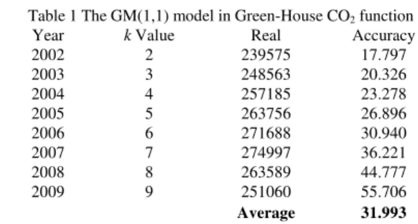
with (GM (1,1)) models. The average accuracy of GM (1,1) is 31.993% in Green-House CO2 function (See Table 1) and it is a weak and inaccurate predictability. (See Table 15)
Table 1 The GM(1,1) model in Green-House CO2 function
Year k Value Real Accuracy
2002 2 239575 17.797
2003 3 248563 20.326
2004 4 257185 23.278
2005 5 263756 26.896
2006 6 271688 30.940
2007 7 274997 36.221
2008 8 263589 44.777
2009 9 251060 55.706
Average 31.993
Table 2 The GM(1,1) model in Green-House Gas function Year k Value Real Accuracy
2001 2 260163 16.165
2002 3 267547 18.295
2003 4 274629 20.744
2004 5 283470 23.390
2005 6 287241 26.866
2006 7 294526 30.496
2007 8 296826 35.219
2008 9 284498 42.767
2009 10 264861 53.466
Average 31.405
The RGM (1,1) approach:
(1). The predictions of Green-House CO2 and Total Gas
with residual (RGM (1,1)). The average accuracy of GM (1,1) is 39.11 in Green-House CO2 function. (See Table 3). The
experimental result is slight improved in this approach. Table 3 The RGM(1,1) model in Green-House CO2 function
Year k Value Real Accuracy
2002 1 239575 17.797
2003 2 248563 26.963
2004 3 257185 30.229
2005 4 263756 34.242
2006 5 271688 38.668
2007 6 274997 44.496
2008 7 263589 54.134
2009 8 251060 66.353
Average 39.110
(2). The average accuracy of RGM (1,1) is 36.468 in Green-House Total Gas function (See Table 4). The experimental results are also getting better in this approach.
Table 4 The GM(1,1) model in Green-House Gas function Year k Value Real Accuracy
2001 1 260163 16.165 2002 2 267547 24.416 2003 3 274629 27.156 2004 4 283470 30.069 2005 5 287241 33.952 2006 6 294526 37.925 2007 7 296826 43.144 2008 8 284498 51.656 2009 9 264861 63.731
Average 36.468
The GM (1,N) approach:
(1). We attempt to setup the GM (1,N) model that need to perform the relation analysis of pollution factors firstly. The relation value of Energy Industry is 0.974 (See Tables 5 & the threshold value is 0.8). It is presented that energy industry is highly related to this prediction mode. (pollution factors:1. Energy Industry; 2. Manufacturing Industry; 3. Transportation Industry; 4. Agricultural Industry; 5. Service Industry; 6. Housing Industry; and 7. Production Industry).
Table 5 The grey relation analysis of Green-House CO2 for (GM (1,N))
Energy
Industry 2 3 4 5 6 7
2002 0.968 0.691 0.672 0.615 0.617 0.619 0.631 2003 0.973 0.670 0.655 0.601 0.603 0.604 0.615 2004 0.963 0.654 0.641 0.588 0.590 0.591 0.602 2005 0.963 0.640 0.632 0.578 0.580 0.581 0.592 2006 0.961 0.629 0.618 0.565 0.569 0.570 0.581 2007 0.963 0.626 0.610 0.560 0.564 0.565 0.575 2008 0.987 0.640 0.626 0.576 0.580 0.581 0.591 2009 1.000 0.658 0.649 0.594 0.599 0.600 0.611
Average 0.974 0.657 0.643 0.590 0.593 0.594 0.605
(2). The relation value of CO2 is 0.939 in Total Gas
function (the threshold value is 0.8) (See Tables 6). It is presented that the CO2 consumption is highly related to this
prediction mode. (1:CO2; 2:CH4; 3:N2O; 4:HFCs; 5:PFCs; and 6:SF6).
Table 6 The grey relation value of Green-House Total Gas for (GM (1,N))
1:CO2 2 3 4 5 6
2001 0.911 0.405 0.409 0.402 0.398 0.397 2002 0.919 0.396 0.401 0.394 0.392 0.390 2003 0.929 0.388 0.393 0.387 0.385 0.384 2004 0.928 0.380 0.385 0.379 0.377 0.376 2005 0.943 0.376 0.382 0.373 0.374 0.374 2006 0.947 0.369 0.375 0.366 0.368 0.368 2007 0.953 0.367 0.373 0.364 0.365 0.366 2008 0.958 0.378 0.384 0.375 0.375 0.376 2009 1.000 0.395 0.395 0.396 0.393 0.394
Average 0.939 0.387 0.391 0.384 0.383 0.382
(3). The predictions of CO2 and Total Gas (GM (1,N)) are
presented as follows. The average accuracy of GM (1,N) is 97.215. (See Table 7) The experimental result is significantly improved in this approach. (Highly accurate forecasting)
Table 7 The average accuracy of Green-House CO2 for (GM (1,N))
Year k Value Real Accuracy
2002 2 239575 92.787 2003 3 248563 96.864 2004 4 257185 97.178 2005 5 263756 98.871 2006 6 271688 99.633 2007 7 274997 98.671 2008 8 263589 97.731 2009 9 251060 98.682
Average 97.215
(4). The average accuracy of GM (1,N) is 98.382 in Total Gas function (See Table 8). The experimental result is the best in this approach. (Highly accurate forecasting (See Table 15)) Table 8 The average accuracy of Green-House Total Gas for (GM (1,N))
Year k Value Real CO2(1) Accuracy
2001 2 260163 230547 95.504
2002 3 267547 239575 97.846
2003 4 274629 248563 98.529
2004 5 283470 257185 98.704
2005 6 287241 263756 99.889
2006 7 294526 271688 99.652
2007 8 296826 274997 99.217
2008 9 284498 263589 99.212
2009 10 264861 251060 96.886
Average 98.382
The RGM (1,N) approach:
(1). The predictions of Green-House CO2 and Total Gas
with residual (RGM (1,N)) mode are presented as follows. The average accuracy of RGM (1,N) is 97.217 in Green-House CO2 function (See Table 9). The experimental
result is similar to the previous model (GM (1,N))CO2.
Table 9 The average accuracy of Green-House CO2 for (RGM (1,N))
Year k Value Real Accuracy
2002 2 239575 92.682 2003 3 248563 96.761 2004 4 257185 97.076 2005 5 263756 98.770 2006 6 271688 99.733 2007 7 274997 98.772 2008 8 263589 97.839 2009 9 251060 98.797
(2). The average accuracy of GM (1,N) is 98.107 in Green-House Total Gas function (See Table 10). The experimental result is similar to the previous model (GM (1,N))Total Gas. (Highly accurate forecasting (See Table 15))
Table 10 The average accuracy of Green-House Total Gas for (RGM (1,N)) Year k Value Real Accuracy
2001 2 260163 95.554 2002 3 267547 97.896 2003 4 274629 98.578 2004 5 283470 98.751 2005 6 287241 99.937 2006 7 294526 99.606 2007 8 296826 99.171 2008 9 284498 99.163 2009 10 264861 96.832
Average 98.107
The simulations of CO2 based in the GM(1,1&1,N); and the
sample period from Taiwan’s industry output data (from 2002 to 2009) was presented to create the original data sequence Xi(0)(t), that is Xi(0)(t) = (239,575; ;251,060). Furthermore, the
AGO series x(1) can be obtained, Xi(1)(t) =
(470,122; . .;300,960). The prediction equations of these research models are shown in Table 11 for prediction outputs. Table 11 The grey prediction equations of Green-House CO2 for grey models
Finally, we obtain the sequence X(t=0) (k) = (222,041; ..,
254,080) as the output of predictive value of Taiwan’s industry in Table 12 and Figure 2. The average accuracy of GM (1,N) is 97.215 in Green-House CO2 function.
Table12 The comparisons of GM models for Green-House CO2 function
Figure 2 The comparisons of GM for Green-House CO2 function
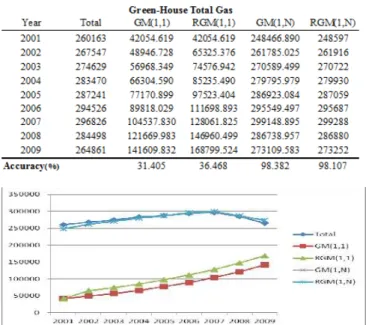
The simulations of Total Gas based in models GM(1,1&1,N); and the sample data were obtained from the Industrial Technology Information from 2001 to 2009. The simulation of Total Gas is performed the prediction equations (see Table 13). The output data was presented to create the original data sequence Xi(0)(t), that is Xi(0)(t) = (260,163; ;
264,861). Furthermore, from the prediction equations (see Table 6), the AGO series Xi(1)(t) can be obtained from the
prediction equations (see Table 13), Xi(1)(t) =
(516,774; ;2770,372).
Table 13 The grey prediction equations of Green-House Total Gas models
The data series can be found as the output of the predictive value of Taiwan’s industries for from 2001 to 2009. Finally, we obtain the prediction value series X(t=0) (k) = (248,597; ..,
273,252) as the best output of predictive value of Taiwan’s industries. The average accuracy of GM (1,N) mode is 98.382 in Green-House Total Gas function.
This study predicts the environment pollution value by using models GM (1,1); RGM (1,1); GM (1,N); and RGM (1,N) models. Real and predicting values were selected to compare the error accuracy of these different models. The experimental conclusions of the predicting model, explained in Table 14 and Figure 3.
Table 14 The comparisons of GM models for Green-House Total Gas function
Table 12 and Figure 2 show a Green-House CO2 function
and Table 14 and Figure 3 present a Green-House Total Gas function. The experimental results disclose that the GM (1,N) model is more accurate than the other two models (GM(1,1) & RGM(1,1)). The average accuracy of GM (1,1) mode (the average accuracy is 31%) is worse than that of RGM (1,1) mode (the average accuracy is 39%). We also find the residual test of these two models improve that they do better than (GM(1,1) & GM(1,N)) models. The residual test values of RGM (1,N) models (the average accuracy is 97% & 98%) (Error<10% Highly accurate forecasting) perform better than GM (1,1) & RGM (1,1) models. Especially, when the GM(1,1) is modified by using a RGM (1,N), the performance of absolute error decrease to 58% & 66%. (<10% Highly accurate forecasting). Hence, it can be concluded that GM (1,1) is not suitable for these prediction models.
After a simulation conclusion, the residual tests were designed as these two experimental decision factors to appraise the performance of the simulation patterns. These standards are defined as Table 15 which denote the actual value, and the predicted value. The lower the residual test values, the more accurate the prediction. Lewis [15] presented the standard levels of MAPE (%) in Table 15.
Table 15 The Standard Levels of MAPE (%) model evaluation
Residual Test :
% 100 ) (
) ( ˆ ) ( )
( (0) (0) (0)
t t t t e
<10% Highly accurate forecasting 10–20% Good forecasting 20–50% Reasonable forecasting >50% Weak and inaccurate predictability
Criteria of MAPE(%) Forecasting ability Source: Lewis [16]
Table 12 & 14 explain the best conclusion (<10% = (1-0.98) for model evaluation that is highly accurate forecasting in these experiments. In forecasting pollution consumptions in Taiwan industries, the accuracy of GM (1,N) and RGM (1,N) models present the better predictions correspondingly.
VI. CONCLUSION
It is very difficult to predict the pollution trends in Taiwan industries. Because the industry pollution is complicated and strongly affected by economic cycles and environmental pollution factors. Consequently, the issue of how to obtain an accurate forecast is very important for the pollution trends in Taiwan industries. Hence, We proposed the models GM (1, 1); RGM (1, 1); GM (1, N) and RGM (1, N) to predict and compare with those of the manufacturing environment data in Taiwan’s industry manufacturers.
The experimental results have disclosed that the GM(1,1) model is inadequate for short-term forecasting. To increase the accuracy of GM (1,1), the residual modification model is applied herein. The applications of these models have confirmed that RGM(1,1) approach appear to perform better than GM (1,1). The GM(1,N) and RGM(1,N) models (the average accuracy is 97% & 98%) obtain higher quality short-term predictions than do the GM(1,1) and RGM(1,1) mode (the average accuracy is 31% & 39%) approaches. Forecasting error results indicate that GM(1,N) mode is suitable for short-term prediction. It can be concluded that the GM(1,N) and RGM(1,N) models are suitable for making
forecasts about Taiwan industry pollution (Energy; Manufacturing; Transportation; Agricultural; Housing; and Production Industry). This work only examines forecasting models to determine which models perform better-quality predictions, and numerous related industries influence each other in Taiwan industries. Grey relational analysis can be applied to determine the relationships of pollution factors among these industries, an area that should be researched further in the future.
REFERENCES
[1] Chao-Chin Chung , Ho-Hsien Chen , Ching-Hua Ting., “Grey prediction fuzzy control for pH processes in the food industry”, Journal of Food Engineering, 96, 2010, pp. 575–582.
[2] Chi-Sheng Shih, Yen-Tseng Hsu, Jerome Yeh, Pin-Chan Lee., “Grey number prediction using the grey modification model with progression technique”, Technological Forecasting & Social Change, Applied Mathematical Modelling35, 2011, pp.1314–1321.
[3] Erdal Kayacan , Okyay Kaynak., “Single-step ahead prediction based on the principle of concatenation using grey predictors”, Expert Systems with Applications, 38, 2011, pp.9499–9505.
[4] Erdal Kayacan a,Baris Ulutas b., “Okyay Kaynak a. Grey system theory-based models in time series prediction”, Expert Systems with Applications, 37, 2010, pp.1784–1789.
[5] Hexiang Liu a, Da-Lin Zhang b., “Analysis and prediction of hazard risks caused by tropical cyclones in Southern China with fuzzy mathematical and grey models”, Applied Mathematical Modelling, 36, 2012, pp.626–637.
[6] Hsu, L. C., "Forecasting the output of integrated circuit industry using genetic algorithm based multivariable grey optimization models", Expert Systems with Applications, 36(4),2009, pp.7898–7903. [7] Hui Jiang . Wenwu He ., “Grey relational grade in local support vector
regression for financial time series prediction”, Expert Systems with Applications, 39, 2012, pp.2256–2262.
[8] Hung, K. C., Chien, C. Y., Wu, K. J., & Hsu, F. Y., "Optimal alpha level setting in GM(1,1) model based on genetic algorithm”, Journal of Grey System, 12(1), 2009, pp.23–32.
[9] J.J. Guo, J.Y. Wu, R.Z. Wang., “A new approach to energy consumption prediction of domestic heat pump water heater based on grey system theory”, Computer Communications, Energy and Buildings43, 2011, pp.1273–1279.
[10] José Angel Barrios, Miguel Torres-Alvarado, Alberto Cavazos., “Neural, fuzzy and Grey-Box modelling for entry temperature prediction in a hot strip mill”, Expert Systems with Applications, Expert Systems with Applications39, 2012, pp.3374–3384.
[11] Li-Chang Hsu, “Using improved grey forecasting models to forecast the output of opto-electronics industry”, Expert Systems with Applications, Expert Systems with Applications 38, 2011, pp.13879– 13885.
[12] Qinbao Song, Martin Shepperd, “Predicting software project effort: A grey relational analysis based method”; Expert Systems with Applications,38,2011, pp.7302–7316.
[13] Shun-Chung Lee, Li-Hsing Shih,“ Forecasting of electricity costs based on an enhanced gray-based learning model: A case study of renewable energy in Taiwan”; Technological Forecasting & Social Change,78,2011, pp.1242–1253.
[14] Xueli An, Dongxiang Jiang, Minghao Zhao, Chao Liu. ,“Short-term prediction of wind power using EMD and chaotic theory”;Commun Nonlinear Sci Numer Simulat,17, 2012, pp.1036–1042.
[15] Yuan-Yeuan Tai , Jenn-Yang Lin , Ming-Shi Chen , Ming-Chyuan Lin., “A grey decision and prediction model for investment in the core competitiveness of product development”, Applied Mathematical Modelling, Technological Forecasting & Social Change78, 2011, pp.1254–1267.