Livros e Materiais Online Evandro Marquesone

(1)

Seamless R and C++ Integration:

Rcpp and RInside

Dirk Eddelbuettel

Debian Project

Joint work with Romain François

Invited seminar presentation

Institute for Statistics and Mathematics

(2)

Preliminaries

(3)

We assume a recent version of

R

so that

(4)

Preliminaries

We assume a recent version of

R

so that

install.packages(c("Rcpp","RInside","inline"))

gets us current versions of the packages

All examples shown should work ’as is’ on Linux, OS X and

Windows

provided a complete

R

development environment

(5)

We assume a recent version of

R

so that

install.packages(c("Rcpp","RInside","inline"))

gets us current versions of the packages

All examples shown should work ’as is’ on Linux, OS X and

Windows

provided a complete

R

development environment

(6)

Preliminaries

We assume a recent version of

R

so that

install.packages(c("Rcpp","RInside","inline"))

gets us current versions of the packages

All examples shown should work ’as is’ on Linux, OS X and

Windows

provided a complete

R

development environment

The

R Installation and Administration

manual is an

excellent start if you need to address the preceding point

In particular, one must use the same compilers used to

build

R

in order to extend or embed the

R

engine

(7)

We assume a recent version of

R

so that

install.packages(c("Rcpp","RInside","inline"))

gets us current versions of the packages

All examples shown should work ’as is’ on Linux, OS X and

Windows

provided a complete

R

development environment

The

R Installation and Administration

manual is an

excellent start if you need to address the preceding point

In particular, one must use the same compilers used to

build

R

in order to extend or embed the

R

engine

However, there is a known issue with the current RInside /

(8)

Outline

1 _{Extending R}

Why ?

The standard API

Inline

2 _Rcpp

Overview

New API

Examples

(9)

(10)

Motivation

Chambers.Software for Data Analysis: Programming with R. Springer, 2008

Chambers (2008) opens chapter 11 (

Interfaces I:

Using C and Fortran)

with these words:

(11)

Chambers.Software for Data Analysis: Programming with R. Springer, 2008

Chambers (2008) opens chapter 11 (

Interfaces I:

(12)

Motivation

Chambers (2008) then proceeds with this rough map of the

road ahead:

(13)

Chambers (2008) then proceeds with this rough map of the

road ahead:

(14)

Motivation

Chambers (2008) then proceeds with this rough map of the

road ahead:

Against:

It’s more work

(15)

Chambers (2008) then proceeds with this rough map of the

road ahead:

Against:

(16)

Motivation

Chambers (2008) then proceeds with this rough map of the

road ahead:

Against:

It’s more work

Bugs will bite

Potential platform

dependency

(17)

Chambers (2008) then proceeds with this rough map of the

road ahead:

Against:

It’s more work

Bugs will bite

Potential platform

dependency

(18)

Motivation

Chambers (2008) then proceeds with this rough map of the

road ahead:

Against:

It’s more work

Bugs will bite

Potential platform

dependency

Less readable software

(19)

Chambers (2008) then proceeds with this rough map of the

road ahead:

Against:

It’s more work

Bugs will bite

Potential platform

dependency

Less readable software

In Favor:

(20)

Motivation

Chambers (2008) then proceeds with this rough map of the

road ahead:

Against:

It’s more work

Bugs will bite

Potential platform

dependency

Less readable software

In Favor:

New and trusted

computations

Speed

(21)

Chambers (2008) then proceeds with this rough map of the

road ahead:

Against:

It’s more work

Bugs will bite

Potential platform

dependency

Less readable software

In Favor:

New and trusted

computations

Speed

(22)

Motivation

Chambers (2008) then proceeds with this rough map of the

road ahead:

Against:

It’s more work

Bugs will bite

Potential platform

dependency

Less readable software

In Favor:

New and trusted

computations

Speed

Object references

(23)

Chambers (2008) then proceeds with this rough map of the

road ahead:

Against:

It’s more work

Bugs will bite

Potential platform

dependency

Less readable software

In Favor:

New and trusted

computations

Speed

Object references

(24)

Motivation

Chambers (2008) then proceeds with this rough map of the

road ahead:

Against:

It’s more work

Bugs will bite

Potential platform

dependency

Less readable software

In Favor:

New and trusted

computations

Speed

Object references

So is the deck stacked against us?

(25)

1 _{Extending R}

Why ?

The standard API

Inline

2 _Rcpp

(26)

Compiled Code: The Basics

R

offers several functions to access compiled code: we focus

on

.C

and

.Call

here. (

R Extensions

, sections 5.2 and 5.9;

Software for Data Analysis

).

(27)

R

offers several functions to access compiled code: we focus

on

.C

and

.Call

here. (

R Extensions

, sections 5.2 and 5.9;

Software for Data Analysis

).

The canonical example is the convolution function:

1 void convolve (double ∗a , i n t ∗na , double ∗b , 2 i n t ∗nb , double ∗ab )

3 {

4 i n t i , j , nab =∗na +∗nb−1 ; 5

6 f o r( i = 0 ; i < nab ; i ++) 7 ab [ i ] = 0 . 0 ;

(28)

Compiled Code: The Basics cont.

The convolution function is called from

R

by

(29)

The convolution function is called from

R

by

1 conv<−function( a , b ) 2 .C( " convolve " , 3 as.double( a ) , 4 as.i n t e g e r(length( a ) ) , 5 as.double( b ) , 6 as.i n t e g e r(length( b ) ) ,

7 ab = double(length( a ) + length( b )−1 ) )$ab

As stated in the manual, one must take care to coerce all the

arguments to the correct

R

storage mode before calling

.C

as

(30)

Example: Running the convolution code via .C

All these files are at

http://dirk.eddelbuettel.com/code/rcppTut

Turn the C source file into a dynamic library using

R CMD SHLIB convolve.C.c

(31)

Turn the C source file into a dynamic library using

R CMD SHLIB convolve.C.c

Load it inside an

R

script or session using

(32)

Example: Running the convolution code via .C

All these files are at

http://dirk.eddelbuettel.com/code/rcppTut

Turn the C source file into a dynamic library using

R CMD SHLIB convolve.C.c

Load it inside an

R

script or session using

dyn.load("convolve.C.so")

Use it via the

.C()

interface as shown on previous slide

(33)

Turn the C source file into a dynamic library using

R CMD SHLIB convolve.C.c

Load it inside an

R

script or session using

dyn.load("convolve.C.so")

Use it via the

.C()

interface as shown on previous slide

All together in a helper file

convolve.C.sh

#!/bin/sh

R CMD SHLIB convolve.C.c

(34)

Compiled Code: The Basics cont.

Using

.Call, the example becomes

(35)

Using

.Call, the example becomes

1 # include <R . h> 2 # include < Rdefines . h> 3

4 extern "C" SEXP convolve2 (SEXP a , SEXP b ) 5 {

6 i n t i , j , na , nb , nab ; 7 double ∗xa , ∗xb , ∗xab ; 8 SEXP ab ;

9

10 PROTECT( a = AS_NUMERIC( a ) ) ; 11 PROTECT( b = AS_NUMERIC( b ) ) ;

12 na = LENGTH( a ) ; nb = LENGTH( b ) ; nab = na + nb−1 ; 13 PROTECT( ab = NEW_NUMERIC( nab ) ) ;

14 xa = NUMERIC_POINTER ( a ) ; xb = NUMERIC_POINTER ( b ) ; 15 xab = NUMERIC_POINTER ( ab ) ;

16 f o r( i = 0 ; i < nab ; i ++) xab [ i ] = 0 . 0 ; 17 f o r( i = 0 ; i < na ; i ++)

18 f o r( j = 0 ; j < nb ; j ++) xab [ i + j ] += xa [ i ] ∗xb [ j ] ; 19 UNPROTECT( 3 ) ;

(36)

Compiled Code: The Basics cont.

Now the call simplifies to just the function name and the vector

arguments—all other handling is done at the C/C++ level:

1

conv

<

−

function

( a , b ) .

C a l l

( " convolve2 " , a , b )

(37)

Now the call simplifies to just the function name and the vector

arguments—all other handling is done at the C/C++ level:

1

conv

<

−

function

( a , b ) .

C a l l

( " convolve2 " , a , b )

In summary, we see that

(38)

Compiled Code: The Basics cont.

Now the call simplifies to just the function name and the vector

arguments—all other handling is done at the C/C++ level:

1

conv

<

−

function

( a , b ) .

C a l l

( " convolve2 " , a , b )

In summary, we see that

there are different entry points

using different calling conventions

(39)

Now the call simplifies to just the function name and the vector

arguments—all other handling is done at the C/C++ level:

1

conv

<

−

function

( a , b ) .

C a l l

( " convolve2 " , a , b )

In summary, we see that

there are different entry points

using different calling conventions

(40)

Example: Running the convolution code via .Call

Turn the C source file into a dynamic library using

R CMD SHLIB convolve.Call.c

(41)

Turn the C source file into a dynamic library using

R CMD SHLIB convolve.Call.c

Load it inside an

R

script or session using

(42)

Example: Running the convolution code via .Call

Turn the C source file into a dynamic library using

R CMD SHLIB convolve.Call.c

Load it inside an

R

script or session using

dyn.load("convolve.Call.so")

Use it via the

.Call()

interface as shown previously

(43)

Turn the C source file into a dynamic library using

R CMD SHLIB convolve.Call.c

Load it inside an

R

script or session using

dyn.load("convolve.Call.so")

Use it via the

.Call()

interface as shown previously

All together in a helper file

convolve.Call.sh

#!/bin/sh

R CMD SHLIB convolve.Call.c

(44)

Outline

1 _{Extending R}

Why ?

The standard API

Inline

2 _Rcpp

Overview

New API

Examples

(45)

inline

is a package by Oleg Sklyar et al that provides the

(46)

Compiled Code: inline

inline

is a package by Oleg Sklyar et al that provides the

function

cfunction

which can wrap Fortran, C or C++ code.

1

## A s i m p l e F o r t r a n example

2

code

<

−

"

3

i n t e g e r i

4

do 1 i =1 , n ( 1 )

5

1 x ( i ) = x ( i )

∗∗

3

6

"

7

cubefn

<

−

c f u n c t i o n ( s i g n a t u r e ( n= " i n t e g e r " , x= " numeric " ) ,

8

code , c o n v e n t i o n = " . F o r t r a n " )

9

x

<

−

as

.

numeric

( 1 : 1 0 )

10

n

<

−

as

.

i n t e g e r

( 1 0 )

11

cubefn ( n , x )

$

x

(47)

inline

is a package by Oleg Sklyar et al that provides the

function

cfunction

which can wrap Fortran, C or C++ code.

1

## A s i m p l e F o r t r a n example

2

code

<

−

"

3

i n t e g e r i

4

do 1 i =1 , n ( 1 )

5

1 x ( i ) = x ( i )

∗∗

3

6

"

7

cubefn

<

−

c f u n c t i o n ( s i g n a t u r e ( n= " i n t e g e r " , x= " numeric " ) ,

8

code , c o n v e n t i o n = " . F o r t r a n " )

9

x

<

−

as

.

numeric

( 1 : 1 0 )

10

n

<

−

as

.

i n t e g e r

( 1 0 )

11

cubefn ( n , x )

$

x

cfunction

takes care of compiling, linking, loading, . . . by

placing the resulting dynamically-loadable object code in the

(48)

Example: Convolution via .C with inline

Using the file

convolve.C.inline.R

1 r e q u i r e( i n l i n e ) 2

3 code<− " i n t i , j , nab =∗na +∗nb−1 ; 4

5 f o r ( i = 0 ; i < nab ; i ++) 6 ab [ i ] = 0 . 0 ;

7

8 f o r ( i = 0 ; i <∗na ; i ++) { 9 f o r ( j = 0 ; j <∗nb ; j ++) 10 ab [ i + j ] += a [ i ] ∗b [ j ] ;

11 }

12 " 13

14 f u n<−c f u n c t i o n ( s i g n a t u r e ( a= " numeric " , na= " numeric " , 15 b= " numeric " , nb= " numeric " , 16 ab= " numeric " ) ,

17 code , language= "C" , c o n v e n t i o n = " . C" ) 18

19 f u n ( 1 : 1 0 , 10 , 1 0 : 1 , 10 , numeric( 1 9 ) )$ab

(49)

1 r e q u i r e( i n l i n e )

2 code<− " i n t i , j , na , nb , nab ; 3 double∗xa , ∗xb , ∗xab ; 4 SEXP ab ;

5

6 PROTECT( a = AS_NUMERIC( a ) ) ; PROTECT( b = AS_NUMERIC( b ) ) ; 7 na = LENGTH( a ) ; nb = LENGTH( b ) ; nab = na + nb−1 ; 8 PROTECT( ab = NEW_NUMERIC( nab ) ) ;

9

10 xa = NUMERIC_POINTER ( a ) ; xb = NUMERIC_POINTER ( b ) ; 11 xab = NUMERIC_POINTER ( ab ) ;

12 f o r ( i = 0 ; i < nab ; i ++) xab [ i ] = 0 . 0 ; 13

14 f o r ( i = 0 ; i < na ; i ++) 15 f o r ( j = 0 ; j < nb ; j ++) 16 xab [ i + j ] += xa [ i ] ∗xb [ j ] ; 17

18 UNPROTECT( 3 ) ; 19 r e t u r n ( ab ) ; " 20

21 f u n<−c f u n c t i o n ( s i g n a t u r e ( a= " numeric " , b= " numeric " ) , 22 code , language= "C" )

23

(50)

Outline

1 _{Extending R}

Why ?

The standard API

Inline

2 _Rcpp

Overview

New API

Examples

(51)

(52)

Compiled Code: Rcpp

In a nutshell:

Rcpp

makes it easier to interface C++ and

R

code.

(53)

In a nutshell:

Rcpp

makes it easier to interface C++ and

R

code.

Using the

.Call

interface, we can use features of the C++

(54)

Compiled Code: Rcpp

In a nutshell:

Rcpp

makes it easier to interface C++ and

R

code.

Using the

.Call

interface, we can use features of the C++

language to automate the tedious bits of the macro-based

C-level interface to

R. One major advantage of using

.Call

is that richer R

objects (vectors, matrices, lists,

. . .

in fact most SEXP

types incl functions, environments etc) can be passed

directly between

R

and C++ without the need for explicit

passing of dimension arguments.

(55)

In a nutshell:

Rcpp

makes it easier to interface C++ and

R

code.

Using the

.Call

interface, we can use features of the C++

language to automate the tedious bits of the macro-based

C-level interface to

R. One major advantage of using

.Call

is that richer R

objects (vectors, matrices, lists,

. . .

in fact most SEXP

types incl functions, environments etc) can be passed

directly between

R

and C++ without the need for explicit

passing of dimension arguments.

By using the C++ class layers, we do not need to

(56)

Compiled Code: Rcpp

In a nutshell:

Rcpp

makes it easier to interface C++ and

R

code.

Using the

.Call

interface, we can use features of the C++

language to automate the tedious bits of the macro-based

C-level interface to

R. One major advantage of using

.Call

is that richer R

objects (vectors, matrices, lists,

. . .

in fact most SEXP

types incl functions, environments etc) can be passed

directly between

R

and C++ without the need for explicit

passing of dimension arguments.

By using the C++ class layers, we do not need to

manipulate the SEXP objects using any of the old-school C

macros.

inline

eases usage, development and testing.

(57)

1 r e q u i r e( i n l i n e ) 2 code<− ’

3 RcppVector <double > xa ( a ) ; 4 RcppVector <double > xb ( b ) ; 5

6 i n t nab = xa . s i z e ( ) + xb . s i z e ( )−1 ; 7 RcppVector <double > xab ( nab ) ;

8 f o r ( i n t i = 0 ; i < nab ; i ++) xab ( i ) = 0 . 0 ; 9

10 f o r ( i n t i = 0 ; i < xa . s i z e ( ) ; i ++) 11 f o r ( i n t j = 0 ; j < xb . s i z e ( ) ; j ++) 12 xab ( i + j ) += xa ( i ) ∗xb ( j ) ; 13

14 RcppResultSet r s ; 15 r s . add ( " ab " , xab ) ; 16 r e t u r n r s . g e t R e t u r n L i s t ( ) ; 17 ’

18

(58)

Outline

1 _{Extending R}

Why ?

The standard API

Inline

2 _Rcpp

Overview

New API

Examples

(59)

(60)

Rcpp: The ’New API’

Rcpp was significantly extended over the last few months to

permit more natural expressions. Consider this comparison

between the R API and the new Rcpp API:

1 SEXP ab ;

2 PROTECT( ab = a l l o c V e c t o r (STRSXP, 2 ) ) ; 3 SET_STRING_ELT ( ab , 0 , mkChar ( " f o o " ) ) ; 4 SET_STRING_ELT ( ab , 1 , mkChar ( " bar " ) ) ; 5 UNPROTECT( 1 ) ;

(61)

Rcpp was significantly extended over the last few months to

permit more natural expressions. Consider this comparison

between the R API and the new Rcpp API:

1 SEXP ab ;

(62)

Rcpp: The ’New API’

Rcpp was significantly extended over the last few months to

permit more natural expressions. Consider this comparison

between the R API and the new Rcpp API:

1 SEXP ab ;

1 C h a r a c t e r V e c t o r ab ( 2 ) ; 2 ab [ 0 ] = " f o o " ; 3 ab [ 1 ] = " bar " ;

Data types, including STL containers and iterators, can be

nested and other niceties. Implicit converters allow us to

combine types:

(63)

Rcpp was significantly extended over the last few months to

permit more natural expressions. Consider this comparison

between the R API and the new Rcpp API:

1 SEXP ab ;

Data types, including STL containers and iterators, can be

nested and other niceties. Implicit converters allow us to

combine types:

1 s t d : : v e c t o r <double> vec ; 2 [ . . . ]

(64)

Rcpp: The ’New API’

Rcpp was significantly extended over the last few months to

permit more natural expressions. Consider this comparison

between the R API and the new Rcpp API:

1 SEXP ab ;

Data types, including STL containers and iterators, can be

nested and other niceties. Implicit converters allow us to

combine types:

1 s t d : : v e c t o r <double> vec ; 2 [ . . . ]

3 L i s t x ( 3 ) ; 4 x [ 0 ] = vec ; 5 x [ 1 ] = " some t e x t " ; 6 x [ 2 ] = 4 2 ;

1 / / With Rcpp 0 . 7 . 1 1 or l a t e r we cando: 2 s t d : : v e c t o r <double> vec ;

3 [ . . . ]

4 L i s t x = L i s t : : c r e a t e ( vec , 5 " some t e x t " ,

6 42) ;

(65)

(66)

Functional programming in both languages

In

R, functional programming is easy:

1 R> data( f a i t h f u l ) ; l a p p l y( f a i t h f u l , summary) 2 $e r u p t i o n s

3 Min . 1 s t Qu . Median Mean 3 r d Qu . Max . 4 1.60 2.16 4.00 3.49 4.45 5.10 5

6 $w a i t i n g

7 Min . 1 s t Qu . Median Mean 3 r d Qu . Max . 8 43.0 58.0 76.0 70.9 82.0 96.0

(67)

In

R, functional programming is easy:

1 R> data( f a i t h f u l ) ; l a p p l y( f a i t h f u l , summary) 2 $e r u p t i o n s

3 Min . 1 s t Qu . Median Mean 3 r d Qu . Max . 4 1.60 2.16 4.00 3.49 4.45 5.10 5

6 $w a i t i n g

7 Min . 1 s t Qu . Median Mean 3 r d Qu . Max . 8 43.0 58.0 76.0 70.9 82.0 96.0

We can do that in C++ as well and pass the

R

function down to

the data that we let the STL

transform

function iterate over:

1 s r c<− ’ Rcpp : : L i s t i n p u t ( data ) ; 2 Rcpp : : F u n c t i o n f ( f u n ) ; 3 Rcpp : : L i s t o u t p u t ( i n p u t . s i z e ( ) ) ;

4 s t d : : t r a n s f o r m ( i n p u t . begin ( ) , i n p u t . end ( ) , o u t p u t . begin ( ) , f ) ; 5 o u t p u t . names ( ) = i n p u t . names ( ) ;

6 r e t u r n o u t p u t ; ’

(68)

Exception handling

Automatic catching and conversion of C++ exceptions:

(69)

R> library(Rcpp); library(inline)

R> cpp <- ’

+

Rcpp::NumericVector x(xs); // automatic conversion from SEXP

+

for (int i=0; i<x.size(); i++) {

+

if (x[i] < 0)

+

throw std::range_error("Non-negative values required");

+

x[i] = log(x[i]);

+

}

+

return x;

// automatic conversion to SEXP

+ ’

R> fun <- cppfunction(signature(xs="numeric"), cpp)

R> fun( seq(2, 5) )

[1] 0.6931 1.0986 1.3863 1.6094

R> fun( seq(5, -2) )

Error in fun(seq(5, -2)) : Non-negative values required

R> fun( LETTERS[1:5] )

(70)

Exception handling: Usage

We attempted to automate forwarding of exceptions from

the C++ layer to the

R

layer.

(71)

We attempted to automate forwarding of exceptions from

the C++ layer to the

R

layer.

This works (thanks to some

gcc

magic) on operating

(72)

Exception handling: Usage

We attempted to automate forwarding of exceptions from

the C++ layer to the

R

layer.

This works (thanks to some

gcc

magic) on operating

system with an X in their name, but not on Windows.

We therefore once again recommend to wrap code with

try {

and

} catch( std::exception &ex) {

forward_exception_to_r(ex);

} catch(...) {

::Rf_error("c++ exception (unknown reason)");

}

(73)

We attempted to automate forwarding of exceptions from

the C++ layer to the

R

layer.

This works (thanks to some

gcc

magic) on operating

system with an X in their name, but not on Windows.

We therefore once again recommend to wrap code with

try {

and

} catch( std::exception &ex) {

forward_exception_to_r(ex);

} catch(...) {

::Rf_error("c++ exception (unknown reason)");

}

Because this is invariant, we provide macros

BEGIN_RCPP

(74)

Exception handling: Usage

We attempted to automate forwarding of exceptions from

the C++ layer to the

R

layer.

This works (thanks to some

gcc

magic) on operating

system with an X in their name, but not on Windows.

We therefore once again recommend to wrap code with

try {

and

} catch( std::exception &ex) {

forward_exception_to_r(ex);

} catch(...) {

::Rf_error("c++ exception (unknown reason)");

}

Because this is invariant, we provide macros

BEGIN_RCPP

and

END_RCPP.

We provide a variant

cppfunction

of

inline::cfunction

which automatically inserts these

at the beginning and end of the code snippets.

(75)

1 _{Extending R}

Why ?

The standard API

Inline

2 _Rcpp

Overview

New API

(76)

Example: Convolution using new Rcpp

Using the file

convolve.Call.Rcpp.new.R

1 r e q u i r e( i n l i n e ) 2

3 code<− ’

4 Rcpp : : NumericVector xa ( a ) ; / / a u t o m a t i c c o n v e r s i o n from SEXP 5 Rcpp : : NumericVector xb ( b ) ;

6

7 i n t n_xa = xa . s i z e ( ) ; 8 i n t n_xb = xb . s i z e ( ) ; 9 i n t nab = n_xa + n_xb−1 ; 10

11 Rcpp : : NumericVector xab ( nab ) ; 12

13 f o r ( i n t i = 0 ; i < n_xa ; i ++) 14 f o r ( i n t j = 0 ; j < n_xb ; j ++) 15 xab [ i + j ] += xa [ i ] ∗xb [ j ] ; 16

17 r e t u r n xab ; / / a u t o m a t i c c o n v e r s i o n t o SEXP 18 ’

19

20 f u n<−c p p f u n c t i o n ( s i g n a t u r e ( a= " numeric " , b= " numeric " ) , code ) 21

22 f u n ( 1 : 1 0 , 1 0 : 1 )

(77)

(78)

Speed comparison

See the directory

Rcpp/examples/ConvolveBenchmarks

In a recently-submitted paper, the following table summarises

the performance of convolution examples:

Implementation

Time in

Relative

millisec

to R API

R API (as benchmark)

32 RcppVector<double>

354

11.1 NumericVector::operator[]

52

1.6 NumericVector::begin

33

1.0 Table 1: Performance for convolution example

(79)

In a recently-submitted paper, the following table summarises

the performance of convolution examples:

Implementation

Time in

Relative

millisec

to R API

R API (as benchmark)

32 RcppVector<double>

354

11.1 NumericVector::operator[]

52

1.6 NumericVector::begin

33

1.0 Table 1: Performance for convolution example

(80)

Another Speed Comparison Example

Regression is a key component of many studies. In

simulations, we often want to run a very large number of

regressions.

(81)

Regression is a key component of many studies. In

simulations, we often want to run a very large number of

regressions.

R

has

lm()

as the general purposes function. It is very

(82)

Another Speed Comparison Example

Regression is a key component of many studies. In

simulations, we often want to run a very large number of

regressions.

R

has

lm()

as the general purposes function. It is very

powerful and returns a rich object—but it is not

lightweight

.

For this purpose,

R

has

lm.fit(). But, this does not

provide all relevant auxiliary data as

e.g.

the standard error

of the estimate.

(83)

Regression is a key component of many studies. In

simulations, we often want to run a very large number of

regressions.

R

has

lm()

as the general purposes function. It is very

powerful and returns a rich object—but it is not

lightweight

.

For this purpose,

R

has

lm.fit(). But, this does not

provide all relevant auxiliary data as

e.g.

the standard error

of the estimate.

For the most recent

Introduction to High-Performance

(84)

Another Speed Comparison Example

Regression is a key component of many studies. In

simulations, we often want to run a very large number of

regressions.

R

has

lm()

as the general purposes function. It is very

powerful and returns a rich object—but it is not

lightweight

.

For this purpose,

R

has

lm.fit(). But, this does not

provide all relevant auxiliary data as

e.g.

the standard error

of the estimate.

For the most recent

Introduction to High-Performance

Computing with R

tutorial, I had written a hybrid R/C/C++

solution using the GNU GSL.

We complement this with a new C++ implementation

around the Armadillo linear algebra classes.

(85)

1 lmGSL<−function( ) { 2 s r c<− ’

3

4 RcppVectorView <double > Yr ( Ysexp ) ; 5 RcppMatrixView <double > Xr ( Xsexp ) ; 6

7 i n t i , j , n = Xr . dim1 ( ) , k = Xr . dim2 ( ) ; 8 double c h i 2 ;

9

10 g s l_m a t r i x ∗X = g s l_m a t r i x_a l l o c ( n , k ) ; 11 g s l_v e c t o r ∗y = g s l_v e c t o r_a l l o c ( n ) ; 12 g s l_v e c t o r ∗c = g s l_v e c t o r_a l l o c ( k ) ; 13 g s l_m a t r i x ∗cov = g s l_m a t r i x_a l l o c ( k , k ) ; 14

15 f o r ( i = 0 ; i < n ; i ++) { 16 f o r ( j = 0 ; j < k ; j ++) {

17 g s l_m a t r i x_s e t ( X , i , j , Xr ( i , j ) ) ; 18 }

19 g s l_v e c t o r_s e t ( y , i , Yr ( i ) ) ; 20 }

21

22 g s l_m u l t i f i t_l i n e a r_workspace ∗wk = 23 g s l_m u l t i f i t_l i n e a r_a l l o c ( n , k ) ; 24 g s l_m u l t i f i t_l i n e a r ( X , y , c , cov ,&chi2 , wk ) ; 25 g s l_m u l t i f i t_l i n e a r_f r e e ( wk ) ;

26 RcppVector <double > S t d E r r ( k ) ;

28 f o r ( i = 0 ; i < k ; i ++) { 29 Coef ( i ) = g s l_ vector _get(c, i ) ; 30 S t d E r r ( i ) =

31 s q r t( g s l_ matrix _get(cov, i , i ) ) ; 32 }

33

34 g s l_ matrix _f r e e ( X ) ; 35 g s l_ vector _f r e e ( y ) ; 36 g s l_ vector _f r e e (c) ; 37 g s l_ matrix _f r e e (cov) ; 38

39 RcppResultSet r s ; 40 r s .add( " c o e f " , Coef ) ; 41 r s .add( " s t d e r r " , S t d E r r ) ; 42

43 r e t u r n = r s . g e t R e t u r n L i s t ( ) ; 44 ’

45 ## t u r n i n t o a f u n c t i o n t h a t R can c a l l 46 ## args redundant on Debian/Ubuntu 47 f u n<−

48 c p p f u n c t i o n ( s i g n a t u r e ( Ysexp =" numeric " , 49 Xsexp =" numeric " ) , src ,

50 i n c l u d e s =

51 " # i n c l u d e < g s l/g s l_m u l t i f i t . h > " , 52 cppargs="−I/u s r/i n c l u d e " ,

(86)

Linear regression via Armadillo: lmArmadillo example

Also see the directory

Rcpp/examples/FastLM

1 l m A r m a d i l l o<−function( ) { 2 s r c<− ’

3 Rcpp : : NumericVector y r ( Ysexp ) ;

4 Rcpp : : NumericVector Xr ( Xsexp ) ; / / a c t u a l l y an n x k m a t r i x 5 s t d : : v e c t o r < i n t > dims = Xr . a t t r ( " dim " ) ;

6 i n t n = dims [ 0 ] , k = dims [ 1 ] ;

7 arma : : mat X ( Xr . begin ( ) , n , k , f a l s e ) ; / / use advanced a r m a d i l l o c o n s t r u c t o r s 8 arma : : c o l v e c y ( y r . begin ( ) , y r . s i z e ( ) ) ;

9 arma : : c o l v e c c o e f = s o l v e ( X , y ) ; / / model f i t

10 arma : : c o l v e c r e s i d = y−X∗c o e f ; / / t o comp . s t d . e r r r o f t h e c o e f f i c i e n t s 11 arma : : mat covmat = t r a n s ( r e s i d )∗r e s i d/( n−k ) ∗arma : : i n v ( arma : : t r a n s ( X )∗X ) ; 12

13 Rcpp : : NumericVector c o e f r ( k ) , s t d e r r e s t r ( k ) ;

14 f o r ( i n t i =0 ; i <k ; i ++) { / / w i t h RcppArmadillo t e m p l a t e c o n v e r t e r s 15 c o e f r [ i ] = c o e f [ i ] ; / / t h i s would n o t be needed b u t we o n l y 16 s t d e r r e s t r [ i ] = s q r t ( covmat ( i , i ) ) ; / / have Rcpp . h here

17 } 18

19 r e t u r n Rcpp : : L i s t : : c r e a t e ( Rcpp : : Named ( " c o e f f i c i e n t s " , c o e f r ) , / / Rcpp 0 . 7 . 1 1 20 Rcpp : : Named ( " s t d e r r " , s t d e r r e s t r ) ) ;

21 ’ 22

23 ## t u r n i n t o a f u n c t i o n t h a t R can c a l l

24 f u n<− c p p f u n c t i o n ( s i g n a t u r e ( Ysexp= " numeric " , Xsexp= " numeric " ) , 25 src , i n c l u d e s = " # i n c l u d e < a r m a d i l l o > " ,

26 cppargs= "−I/u s r/i n c l u d e " , l i b a r g s = "−l a r m a d i l l o " ) 27 }

(87)

fastLm

in the new

RcppArmadillo

release does even better:

1 # include < RcppArmadillo . h>

2 extern "C" SEXP fastLm (SEXP ys , SEXP Xs ) { 3 t r y {

4 Rcpp : : NumericVector y r ( ys ) ; / / c r e a t e s Rcpp v e c t o r from SEXP 5 Rcpp : : N u m e r i c M a t r i x Xr ( Xs ) ; / / c r e a t e s Rcpp m a t r i x from SEXP 6 i n t n = Xr . nrow ( ) , k = Xr . n c o l ( ) ;

7

8 arma : : mat X ( Xr . begin ( ) , n , k , f a l s e) ; / / reuses memory and a v o i d s e x t r a copy 9 arma : : c o l v e c y ( y r . begin ( ) , y r . s i z e ( ) , f a l s e) ;

10

11 arma : : c o l v e c c o e f = arma : : s o l v e ( X , y ) ; / / f i t model y ~X 12 arma : : c o l v e c r e s = y−X∗c o e f ; / / r e s i d u a l s 13

14 double s2 = s t d : : i n n e r_p r o d u c t ( r e s . begin ( ) , r e s . end ( ) , r e s . begin ( ) ,double( ) )/( n−k ) ; 15 / / s t d . e r r o r s o f c o e f f i c i e n t s

16 arma : : c o l v e c s t d e r r = arma : : s q r t ( s2∗arma : : diagvec ( arma : : i n v ( arma : : t r a n s ( X )∗X ) ) ) ; 17

18 r e t u r n Rcpp : : L i s t : : c r e a t e ( Rcpp : : Named ( " c o e f f i c i e n t s " ) = coef , 19 Rcpp : : Named ( " s t d e r r " ) = s t d e r r , 20 Rcpp : : Named ( " d f " ) = n−k ) ; 21 } catch( s t d : : e x c e p t i o n &ex ) {

22 f o r w a r d_e x c e p t i o n_t o_r ( ex ) ; 23 } catch( . . . ) {

(88)

Linear regression via GNU GSL: RcppGSL

See

fastLm

in the RcppGSL package (on R-Forge)

We also wrote

fastLm

in a new package

RcppGSL:

1 extern "C" SEXP fastLm (SEXP ys , SEXP Xs ) { 2 BEGIN_RCPP

3 RcppGSL : : v e c t o r <double> y = ys ; / / c r e a t e g s l data s t r u c t u r e s from SEXP 4 RcppGSL : : m a t r i x <double> X = Xs ;

5 i n t n = X . nrow ( ) , k = X . n c o l ( ) ; 6 double c h i s q ;

7 RcppGSL : : v e c t o r <double> c o e f ( k ) ; / / t o h o l d t h e c o e f f i c i e n t v e c t o r 8 RcppGSL : : m a t r i x <double> cov ( k , k ) ; / / and t h e c o v a r i a n c e m a t r i x 9 / / t h e a c t u a l f i t r e q u i r e s working memory we a l l o c a t e and f r e e 10 g s l_m u l t i f i t_l i n e a r_workspace ∗work = g s l_m u l t i f i t_l i n e a r_a l l o c ( n , k ) ; 11 g s l_m u l t i f i t_l i n e a r ( X , y , coef , cov , &chis q , work ) ;

12 g s l_m u l t i f i t_l i n e a r_f r e e ( work ) ; 13 / / e x t r a c t t h e d i a g o n a l as a v e c t o r view 14 g s l_v e c t o r_view d i a g = g s l_m a t r i x_d i a g o n a l ( cov ) ;

15 / / c u r r e n t l y t h e r e i s not a more d i r e c t i n t e r f a c e i n Rcpp : : NumericVector 16 / / t h a t t a k e s advantage o f wrap , so we have t o do i t i n two s t e p s 17 Rcpp : : NumericVector s t d e r r ; s t d e r r = d i a g ;

18 s t d : : t r a n s f o r m ( s t d e r r . begin ( ) , s t d e r r . end ( ) , s t d e r r . begin ( ) , s q r t ) ; 19 Rcpp : : L i s t r e s = Rcpp : : L i s t : : c r e a t e ( Rcpp : : Named ( " c o e f f i c i e n t s " ) = coef , 20 Rcpp : : Named ( " s t d e r r " ) = s t d e r r , 21 Rcpp : : Named ( " d f " ) = n−k ) ;

22 / / f r e e a l l t h e GSL v e c t o r s and m a t r i c e s−−as these are r e a l l y C data s t r u c t u r e s 23 / / we cannot t a k e advantage o f a u t o m a t i c memory management

24 c o e f . f r e e ( ) ; cov . f r e e ( ) ; y . f r e e ( ) ; X . f r e e ( ) ; 25 r e t u r n r e s ; / / r e t u r n t h e r e s u l t l i s t t o R 26 END_RCPP

27 }

(89)

lm lm.fit lmGSL lmArmadillo Comparison of R and linear model fit routines

time in milliseconds

0 50 100 150 200 250

longley (16 x 7 obs)

simulated (10000 x 3)

The small

_longley

example exhibits less

variability between

methods, but the larger

data set shows the gains

more clearly.

(90)

Another Rcpp example (cont.)

lm lm.fit lmGSL lmArmadillo Comparison of R and linear model fit routines

ratio to lm() baseline

0

10

20

30

40 longley (16 x 7 obs)

simulated (10000 x 3)

Source: Our calculations, seeexamples/FastLM/inRcpp.

By dividing the

lm

time by

the respective times, we

obtain the ’possible gains’

from switching.

One caveat,

measurements depends

critically on the size of the

data as well as the cpu

and libraries that are

used.

(91)

(92)

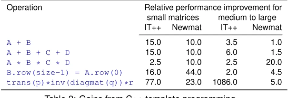
Possible gains from template meta-programming

Armadillo uses delayed evaluation (via recursive template and

template meta-programming) to combine several operations

into one expression reducing / eliminating temporary objects.

Operation

Relative performance improvement for

small matrices

medium to large

IT++

Newmat

IT++

Newmat

A + B

15.0

10.0

3.5

1.0 A + B + C + D

15.0

10.0

6.0

1.5 A * B * C * D

2.5

10.0

2.5

20.0 B.row(size-1) = A.row(0)

16.0

44.0

2.0

4.5 trans(p)inv(diagmat(q))r

77.0

23.0 1086.0

5.0 Table 2: Gains from C++ template programming

Seehttp://arma.sourceforge.net/speed.htmlfor details.

(93)

1 _{Extending R}

Why ?

The standard API

Inline

2 _Rcpp

(94)

From RApache to littler to RInside

See the file

RInside/standard/rinside_sample0.cpp

Jeff Horner’s work on

RApache

lead to joint work in

littler,

a scripting / cmdline front-end. As it embeds

R

and simply

’feeds’ the REPL loop, the next step was to embed R in proper

C++ classes:

RInside.

(95)

Jeff Horner’s work on

RApache

lead to joint work in

littler,

a scripting / cmdline front-end. As it embeds

R

and simply

’feeds’ the REPL loop, the next step was to embed R in proper

C++ classes:

RInside.

1 # include < R I n s i d e . h> / / f o r t h e embedded R v i a R I n s i d e 2

3 i n t main (i n t argc , char ∗argv [ ] ) { 4

5 R I n s i d e R( argc , argv ) ; / / c r e a t e an embedded R i n s t a n c e 6

7 R [ " t x t " ] = " H e l l o , w o r l d!\ n " ; / / a s s i g n a char∗ ( s t r i n g ) t o ’ t x t ’ 8

9 R . parseEvalQ ( " c a t ( t x t ) " ) ; / / e v a l t h e i n i t s t r i n g , i g n o r i n g any r e t u r n s 10

(96)

Another simple example

See

RInside/standard/rinside_sample8.cpp

(in SVN, older version in pkg)

This example shows some of the new assignment and

converter code:

1

8 R [ " x " ] = 10 ; 9 R [ " y " ] = 20 ; 10

11 R . parseEvalQ ( " z<−x + y " ) ; 12

13 i n t sum = R [ " z " ] ; 14

15 s t d : : c o u t << " 10 + 20 = " << sum << s t d : : e n d l ; 16 e x i t ( 0 ) ;

17 }

(97)

1 # include < R I n s i d e . h> / / f o r t h e embedded R v i a R I n s i d e 2 # include <iomanip >

3 i n t main (i n t argc , char ∗argv [ ] ) {

4 R I n s i d e R( argc , argv ) ; / / c r e a t e an embedded R i n s t a n c e 5 SEXP ans ;

6 R . parseEvalQ ( " suppressMessages ( l i b r a r y ( f P o r t f o l i o ) ) " ) ; 7 t x t = " lppData<−100∗LPP2005 . RET [ , 1 : 6 ] ; "

8 " ewSpec<− p o r t f o l i o S p e c ( ) ; nAssets<−n c o l ( lppData ) ; " ; 9 R . pa rse Ev al ( t x t , ans ) ; / / prepare problem

10 const doubledvec [ 6 ] = { 0 . 1 , 0 . 1 , 0 . 1 , 0 . 1 , 0 . 3 , 0 . 3 } ; / / w e i g h t s 11 const s t d : : v e c t o r <double> w( dvec , &dvec [ 6 ] ) ;

12 R . a s s i g n ( w, " w e i g ht s v e c " ) ; / / a s s i g n STL vec t o R ’ s ’ w e i g h ts v e c ’ 13

14 R . parseEvalQ ( " s e t W ei g h t s ( ewSpec )<− w e ig h t s v ec " ) ;

15 t x t = " e w P o r t f o l i o<− f e a s i b l e P o r t f o l i o ( data = lppData , spec = ewSpec , " 16 " c o n s t r a i n t s = \ " LongOnly \ " ) ; " 17 " p r i n t ( e w P o r t f o l i o ) ; "

18 " vec<−getCovRiskBudgets ( e w P o r t f o l i o @ p o r t f o l i o ) " ;

19 ans = R . pa rse Ev al ( t x t ) ; / / a s s i g n covRiskBudget w e i g h t s t o ans 20 Rcpp : : NumericVector V ( ans ) ; / / c o n v e r t SEXP v a r i a b l e t o an RcppVector 21

22 ans = R . pa rse Ev al ( " names ( vec ) " ) ; / / a s s i g n columns names t o ans 23 Rcpp : : C h a r a c t e r V e c t o r n ( ans ) ;

24

25 f o r ( i n t i =0 ; i <names . s i z e ( ) ; i ++) {

(98)

And another

parallel

example

See the file

RInside/mpi/rinside_mpi_sample2.cpp

1 / / MPI C++ API v e r s i o n o f f i l e c o n t r i b u t e d by J i a n p i n g Hua 2

3 # include <mpi . h> / / mpi header

8 MPI : : I n i t ( argc , argv ) ; / / mpi i n i t i a l i z a t i o n 9 i n t myrank = MPI : :COMM_WORLD. Get_rank ( ) ; / / o b t a i n c u r r e n t node rank 10 i n t nodesize = MPI : :COMM_WORLD. Get_s i z e ( ) ; / / o b t a i n t o t a l nodes r u n n i n g . 11

14 s t d : : s t r i n g s t r e a m t x t ;

15 t x t << " H e l l o from node " << myrank / / node i n f o r m a t i o n 16 << " o f " << nodesize << " nodes!" << s t d : : e n d l ;

17 R . a s s i g n ( t x t . s t r ( ) , " t x t " ) ; / / a s s i g n s t r i n g t o R v a r i a b l e ’ t x t ’ 18

19 s t d : : s t r i n g e v a l s t r = " c a t ( t x t ) " ; / / show node i n f o r m a t i o n

20 R . parseEvalQ ( e v a l s t r ) ; / / e v a l t h e s t r i n g , i g n . any r e t u r n s 21

22 MPI : : F i n a l i z e ( ) ; / / mpi f i n a l i z a t i o n 23

24 e x i t ( 0 ) ; 25 }

(99)

(100)

RInside workflow

C++ programs compute, gather or aggregate raw data.

Data is saved and analysed before a new ’run’ is launched.

(101)

C++ programs compute, gather or aggregate raw data.

Data is saved and analysed before a new ’run’ is launched.

(102)

RInside workflow

C++ programs compute, gather or aggregate raw data.

Data is saved and analysed before a new ’run’ is launched.

With

RInside

we now skip a step:

collect data in a vector or matrix

(103)

C++ programs compute, gather or aggregate raw data.

Data is saved and analysed before a new ’run’ is launched.

With

RInside

we now skip a step:

collect data in a vector or matrix

(104)

RInside workflow

C++ programs compute, gather or aggregate raw data.

Data is saved and analysed before a new ’run’ is launched.

With

RInside

we now skip a step:

collect data in a vector or matrix

pass data to

R

— easy thanks to

Rcpp

wrappers

pass one or more short ’scripts’ as strings to

R

to evaluate

(105)

C++ programs compute, gather or aggregate raw data.

Data is saved and analysed before a new ’run’ is launched.

With

RInside

we now skip a step:

collect data in a vector or matrix

pass data to

R

— easy thanks to

Rcpp

wrappers

pass one or more short ’scripts’ as strings to

R

to evaluate

pass data back to C++ programm — easy thanks to

Rcpp

(106)

RInside workflow

C++ programs compute, gather or aggregate raw data.

Data is saved and analysed before a new ’run’ is launched.

With

RInside

we now skip a step:

collect data in a vector or matrix

pass data to

R

— easy thanks to

Rcpp

wrappers

pass one or more short ’scripts’ as strings to

R

to evaluate

pass data back to C++ programm — easy thanks to

Rcpp

converters

resume main execution based on new results

(107)

C++ programs compute, gather or aggregate raw data.

Data is saved and analysed before a new ’run’ is launched.

With

RInside

we now skip a step:

collect data in a vector or matrix

pass data to

R

— easy thanks to

Rcpp

wrappers

pass one or more short ’scripts’ as strings to

R

to evaluate

pass data back to C++ programm — easy thanks to

Rcpp

converters

resume main execution based on new results

(108)

RInside workflow

C++ programs compute, gather or aggregate raw data.

Data is saved and analysed before a new ’run’ is launched.

With

RInside

we now skip a step:

collect data in a vector or matrix

pass data to

R

— easy thanks to

Rcpp

wrappers

pass one or more short ’scripts’ as strings to

R

to evaluate

pass data back to C++ programm — easy thanks to

Rcpp

converters

resume main execution based on new results

A number of simple examples ship with

RInside

nine

different examples in

examples/standard

(109)

C++ programs compute, gather or aggregate raw data.

Data is saved and analysed before a new ’run’ is launched.

With

RInside

we now skip a step:

collect data in a vector or matrix

pass data to

R

— easy thanks to

Rcpp

wrappers

pass one or more short ’scripts’ as strings to

R

to evaluate

pass data back to C++ programm — easy thanks to

Rcpp

converters

resume main execution based on new results

A number of simple examples ship with

RInside

nine

different examples in

examples/standard

(110)

Outline

1 _{Extending R}

Why ?

The standard API

Inline

2 _Rcpp

Overview

New API

Examples

(111)

Quoting from the page at Google Code:

(112)

About Google ProtoBuf

Quoting from the page at Google Code:

Protocol buffers are a flexible, efficient, automated mechanism for

serializing structured data—think XML, but smaller, faster, and

simpler.

You define how you want your data to be structured once, then

you can use special generated source code to easily write and

read your structured data to and from a variety of data streams

and using a variety of languages.

(113)

Quoting from the page at Google Code:

Protocol buffers are a flexible, efficient, automated mechanism for

serializing structured data—think XML, but smaller, faster, and

simpler.

You define how you want your data to be structured once, then

you can use special generated source code to easily write and

read your structured data to and from a variety of data streams

and using a variety of languages.

You can even update your data structure without breaking

deployed programs that are compiled against the "old" format.

(114)

Google ProtoBuf

1 R> l i b r a r y( RProtoBuf ) ## l o a d t h e package

2 R> r e a d P r o t o F i l e s ( " addressbook . p r o t o " ) ## a c q u i r e p r o t o b u f i n f o r m a t i o n 3 R> bob<−new( t u t o r i a l . Person , ## c r e a t e new o b j e c t

4 + e m a i l = " bob@example . com " , 5 + name = " Bob " ,

6 + i d = 123 )

7 R> w r i t e L i n e s ( bob$t o S t r i n g ( ) ) ## s e r i a l i z e t o s t d o u t 8 name : " Bob "

9 i d : 123

10 e m a i l : " bob@example . com " 11

12 R> bob$e m a i l ## access and/o r o v e r r i d e 13 [ 1 ] " bob@example . com "

14 R> bob$i d <−5 15 R> bob$i d 16 [ 1 ] 5 17

18 R> s e r i a l i z e ( bob , " person . pb " ) ## s e r i a l i z e t o compact b i n a r y f o r m a t