R
IN A NUTSHELL
Joseph Adler
R in a Nutshell
by Joseph Adler
Copyright © 2010 Joseph Adler. All rights reserved. Printed in the United States of America.
Published by O’Reilly Media, Inc., 1005 Gravenstein Highway North, Sebastopol, CA 95472.
O’Reilly books may be purchased for educational, business, or sales promotional use. Online editions are also available for most titles (http://my.safaribooksonline.com). For more infor-mation, contact our corporate/institutional sales department: (800) 998-9938 or [email protected].
Editor: Mike Loukides
Production Editor: Sumita Mukherji Production Services: Newgen North
America, Inc.
Cover Designer: Karen Montgomery Interior Designer: David Futato Illustrator: Robert Romano
Printing History:
December 2009: First Edition.
Nutshell Handbook, the Nutshell Handbook logo, and the O’Reilly logo are registered trade-marks of O’Reilly Media, Inc. R in a Nutshell, the image of a harpy eagle, and related trade dress are trademarks of O’Reilly Media, Inc.
Many of the designations used by manufacturers and sellers to distinguish their products are claimed as trademarks. Where those designations appear in this book, and O’Reilly Media, Inc., was aware of a trademark claim, the designations have been printed in caps or initial caps.
While every precaution has been taken in the preparation of this book, the publisher and author assume no responsibility for errors or omissions, or for damages resulting from the use of the information contained herein.
TM
This book uses RepKover™, a durable and flexible lay-flat binding.
ISBN: 978-0-596-80170-0
Table of Contents
Preface . . . xv
Part I. R Basics
1. Getting and Installing R . . . 3
R Versions 3
Getting and Installing Interactive R Binaries 3
Windows 4
Mac OS X 5
Linux and Unix Systems 5
2. The R User Interface . . . 7
The R Graphical User Interface 7
Windows 8
Mac OS X 8
Linux and Unix 8
The R Console 11
Command-Line Editing 13
Batch Mode 13
Using R Inside Microsoft Excel 14
Other Ways to Run R 15
3. A Short R Tutorial . . . 17
Basic Operations in R 17
Functions 19
Variables 20
Introduction to Data Structures 22
Objects and Classes 25
Models and Formulas 26
Charts and Graphics 28
Getting Help 32
4. R Packages . . . 35
An Overview of Packages 35
Listing Packages in Local Libraries 36
Loading Packages 38
Loading Packages on Windows and Linux 38
Loading Packages on Mac OS X 38
Exploring Package Repositories 39
Exploring Packages on the Web 40
Finding and Installing Packages Inside R 40
Custom Packages 43
Creating a Package Directory 43
Building the Package 45
Part II. The R Language
5. An Overview of the R Language . . . 49
Expressions 49
Objects 50
Symbols 50
Functions 50
Objects Are Copied in Assignment Statements 52
Everything in R Is an Object 52
Special Values 53
NA 53
Inf and -Inf 53
NaN 54
NULL 54
Coercion 54
The R Interpreter 55
Seeing How R Works 57
6. R Syntax . . . 61
Constants 61
Numeric Vectors 61
Character Vectors 62
Symbols 63
Operators 64
Order of Operations 65
Assignments 67
Separating Expressions 67
Parentheses 68
Curly Braces 68
Control Structures 69
Conditional Statements 69
Loops 70
Accessing Data Structures 72
Data Structure Operators 73
Indexing by Integer Vector 73
Indexing by Logical Vector 76
Indexing by Name 76
R Code Style Standards 77
7. R Objects . . . 79
Primitive Object Types 79
Vectors 82
Lists 83
Other Objects 84
Matrices 84
Arrays 84
Factors 85
Data Frames 87
Formulas 88
Time Series 89
Shingles 91
Dates and Times 91
Connections 92
Attributes 92
Class 95
8. Symbols and Environments . . . 97
Symbols 97
Working with Environments 98
The Global Environment 99
Environments and Functions 100
Working with the Call Stack 100
Evaluating Functions in Different Environments 101
Adding Objects to an Environment 103
Exceptions 104
Signaling Errors 104
Catching Errors 105
9. Functions . . . 107
The Function Keyword 107
Arguments 107
Return Values 109
Functions As Arguments 109
Anonymous Functions 110
Properties of Functions 111
Argument Order and Named Arguments 113
Side Effects 114
Changes to Other Environments 114
Input/Output 115
Graphics 115
10. Object-Oriented Programming . . . 117
Overview of Object-Oriented Programming in R 118
Key Ideas 118
Implementation Example 119
Object-Oriented Programming in R: S4 Classes 125
Defining Classes 125
New Objects 126
Accessing Slots 126
Working with Objects 127
Creating Coercion Methods 127
Methods 128
Managing Methods 129
Basic Classes 130
More Help 130
Old-School OOP in R: S3 131
S3 Classes 131
S3 Methods 132
Using S3 Classes in S4 Classes 133
Finding Hidden S3 Methods 133
11. High-Performance R . . . 135
Use Built-in Math Functions 135
Use Environments for Lookup Tables 136
Use a Database to Query Large Data Sets 136
Preallocate Memory 137
Monitor How Much Memory You Are Using 137
Monitoring Memory Usage 137
Increasing Memory Limits 138
Cleaning Up Objects 138
Functions for Big Data Sets 139
Parallel Computation with R 139
High-Performance R Binaries 140
Revolution R 140
Part III. Working with Data
12. Saving, Loading, and Editing Data . . . 147
Entering Data Within R 147
Entering Data Using R Commands 147
Using the Edit GUI 148
Saving and Loading R Objects 151
Saving Objects with save 151
Importing Data from External Files 152
Text Files 152
Other Software 161
Exporting Data 161
Importing Data from Databases 162
Export Then Import 162
Database Connection Packages 162
RODBC 163
DBI 173
TSDBI 178
13. Preparing Data . . . 179
Combining Data Sets 179
Pasting Together Data Structures 180
Merging Data by Common Fields 183
Transformations 185
Reassigning Variables 185
The Transform Function 185
Applying a Function to Each Element of an Object 186
Binning Data 189
Shingles 189
Cut 190
Combining Objects with a Grouping Variable 191
Subsets 191
Bracket Notation 192
subset Function 192
Random Sampling 193
Summarizing Functions 194
tapply, aggregate 194
Aggregating Tables with rowsum 197
Counting Values 198
Reshaping Data 200
Data Cleaning 205
Finding and Removing Duplicates 206
Sorting 206
14. Graphics . . . 211
An Overview of R Graphics 211
Scatter Plots 212
Plotting Time Series 218
Bar Charts 219
Pie Charts 223
Plotting Categorical Data 224
Three-Dimensional Data 229
Plotting Distributions 237
Box Plots 240
Graphics Devices 243
Customizing Charts 244
Common Arguments to Chart Functions 244
Graphical Parameters 244
Basic Graphics Functions 254
15. Lattice Graphics . . . 263
History 263
An Overview of the Lattice Package 264
How Lattice Works 264
A Simple Example 264
Using Lattice Functions 266
Custom Panel Functions 268
High-Level Lattice Plotting Functions 268
Univariate Trellis Plots 269
Bivariate Trellis Plots 293
Trivariate Plots 301
Other Plots 306
Customizing Lattice Graphics 308
Common Arguments to Lattice Functions 308
trellis.skeleton 309
Controlling How Axes Are Drawn 310
Parameters 311
plot.trellis 315
strip.default 316
simpleKey 317
Low-Level Functions 318
Low-Level Graphics Functions 318
Panel Functions 318
Part IV. Statistics with R
16. Analyzing Data . . . 323
Summary Statistics 323
Principal Components Analysis 328
Factor Analysis 332
Bootstrap Resampling 333
17. Probability Distributions . . . 335
Normal Distribution 335
Common Distribution-Type Arguments 338
Distribution Function Families 338
18. Statistical Tests . . . 343
Continuous Data 343
Normal Distribution-Based Tests 344
Distribution-Free Tests 357
Discrete Data 360
Proportion Tests 360
Binomial Tests 361
Tabular Data Tests 362
Distribution-Free Tabular Data Tests 368
19. Power Tests . . . 369
Experimental Design Example 369
t-Test Design 370
Proportion Test Design 371
ANOVA Test Design 372
20. Regression Models . . . 373
Example: A Simple Linear Model 373
Fitting a Model 375
Helper Functions for Specifying the Model 376
Getting Information About a Model 376
Refining the Model 382
Details About the lm Function 382
Assumptions of Least Squares Regression 384
Robust and Resistant Regression 386
Subset Selection and Shrinkage Methods 387
Stepwise Variable Selection 388
Ridge Regression 389
Lasso and Least Angle Regression 390
Principal Components Regression and Partial Least Squares
Regression 391
Nonlinear Models 392
Generalized Linear Models 392
Nonlinear Least Squares 395
Survival Models 396
Smoothing 401
Splines 401
Fitting Polynomial Surfaces 403
Kernel Smoothing 404
Machine Learning Algorithms for Regression 405
Regression Tree Models 406
MARS 418
Neural Networks 423
Project Pursuit Regression 427
Generalized Additive Models 430
Support Vector Machines 432
21. Classification Models . . . 435
Linear Classification Models 435
Logistic Regression 435
Linear Discriminant Analysis 440
Log-Linear Models 444
Machine Learning Algorithms for Classification 445
k Nearest Neighbors 445
Classification Tree Models 446
Neural Networks 450
SVMs 451
Random Forests 451
22. Machine Learning . . . 453
Market Basket Analysis 453
Clustering 458
Distance Measures 458
Clustering Algorithms 459
23. Time Series Analysis . . . 463
Autocorrelation Functions 463
Time Series Models 464
24. Bioconductor . . . 469
An Example 469
Loading Raw Expression Data 470
Loading Data from GEO 474
Matching Phenotype Data 476
Analyzing Expression Data 477
Key Bioconductor Packages 481
Data Structures 485
eSet 485
AssayData 487
AnnotatedDataFrame 487
Other Classes Used by Bioconductor Packages 489
Where to Go Next 490
Resources Outside Bioconductor 490
Vignettes 490
Courses 491
Books 491
Appendix: R Reference . . . 493
Bibliography . . . 591
Index . . . 593
Preface
It’s been 10 years since I was first introduced to R. Back then, I was a young product development manager at DoubleClick, a company that sells advertising software for managing online ad sales. I was working on inventory prediction: estimating the number of ad impressions that could be sold for a given search term, web page, or demographic characteristic. I wanted to play with the data myself, but we couldn’t afford a piece of expensive software like SAS or MATLAB. I looked around for a little while, trying to find an open source statistics package, and stumbled on R. Back then, R was a bit rough around the edges, and was missing a lot of the features it has today (like fancy graphics and statistics functions). But R was intuitive and easy to use; I was hooked. Since that time, I’ve used R to do many different things: esti-mate credit risk, analyze baseball statistics, and look for Internet security threats. I’ve learned a lot about data, and matured a lot as a data analyst.
R, too, has matured a great deal over the past 10 years. R is used at the world’s largest technology companies (including Google, Microsoft, and Facebook), the largest pharmaceutical companies (including Johnson & Johnson, Merck, and Pfizer), and at hundreds of other companies. It’s used in statistics classes at universities around the world and by statistics researchers to try new techniques and algorithms.
Why I Wrote This Book
This book is designed to be a concise guide to R. It’s not intended to be a book about statistics or an exhaustive guide to R. In this book, I tried to show all the things that R can do and to give examples showing how to do them. This book is designed to be a good desktop reference.
I wrote this book because I like R. R is fun and intuitive in ways that other solutions are not. You can do things in a few lines of R that could take hours of struggling in a spreadsheet. Similarly, you can do things in a few lines of R that could take pages of Java code (and hours of Java coding). There are some excellent books on R, but
I couldn’t find an inexpensive book that gave an overview of everything you could do in R. I hope this book helps you use R.
When Should You Use R?
I think R is a great piece of software, but it isn’t the right tool for every problem. Clearly, it would be ridiculous to write a video game in R, but it’s not even the best tool for all data problems.
R is very good at plotting graphics, analyzing data, and fitting statistical models using data that fits in the computer’s memory. It’s not as good at storing data in compli-cated structures, efficiently querying data, or working with data that doesn’t fit in the computer’s memory.
Typically, I use a tool like Perl to preprocess large files before using them in R. It’s technically possible to use R for these problems (by reading files one line at a time and using R’s regular expression support), but it’s pretty awkward. To hold large data files, I usually use a database like MySQL, PostgreSQL, SQLite, or Oracle (when someone else is paying the license fee).
R License Terms
R is an open source software package, licensed under the GNU General Public Li-cense (GPL).* This means that you can install R for free on most desktop and server
machines. (Comparable commercial software packages sell for hundreds or thou-sands of dollars.) If R were a poor substitute for the commercial software packages, this might have limited appeal. However, I think R is better than its commercial counterparts in many respects.
Capability
You can find implementations for hundreds (maybe thousands) of statistical and data analysis algorithms in R. No commercial package offers anywhere near the scope of functionality available through the Comprehensive R Archive Net-work (CRAN).
Community
There are now hundreds of thousands (if not millions) of R users worldwide. By using R, you can be sure that you’re using the same software that your col-leagues are using.
Performance
R’s performance is comparable, or superior, to most commercial analysis pack-ages. R requires you to load data sets into memory before processing. If you have enough memory to hold the data, R can run very quickly. Luckily, memory is cheap. You can buy 32 GB of server RAM for less than the cost of a single desktop license of a comparable piece of commercial statistical software.
Examples
I have tried to provide many unique examples in this book, illustrating how to use different functions in R. I deliberately decided to use new and original examples, and not to rely on the data sets included with R. When I’m trying to solve a problem, I try to find examples of similar solutions. There are already good examples for many functions in the R help files. I tried to provide new examples to help users figure out how to solve their problems quickly. The examples are available by from O’Reilly Media at http://oreilly.com/catalog/9780596801700.
Additionally, the example data is also available through CRAN as an R package. To install the nutshell package, type the following command on the R console:
install.packages("nutshell")
How This Book Is Organized
I’ve broken this book into five parts:• Part I, R Basics, covers the basics of getting and running R. It’s designed to help get you up and running if you’re a new user, including a short tour of the many things you can do with R.
• Part II, The R Language, discusses the R language in detail. This section picks up where the first section leaves off, describing the R language in detail. • Part III, Working with Data, covers data processing in R: loading data into R,
transforming data, summarizing data, and plotting data. Summary statistics and charts are an important part of statistical analysis, but many laypeople don’t think of these things as statistical analysis. So, I cover these topics without using too much math in order to keep them accessible.
• Part IV, Statistics with R, covers statistical tests and models in R.
• Finally, I included an Appendix describing functions and data sets included with the base distribution of R.
If you are new to R, install R and start with Chapter 3. Next, take a look at Chap-ter 5 to learn some of the rules of the R language. If you plan to use R for plotting, statistical tests, or statistical models, take a look at the appropriate chapter. Make sure you look at the first few sections of the chapter, because these provide an over-view of how all the related functions work. (For example, don’t skip straight to “Random forests for regression” on page 416 without reading “Example: A Simple Linear Model” on page 373.)
Conventions Used in This Book
The following typographical conventions are used in this book: Italic
Indicates new terms, URLs, email addresses, filenames, and file extensions. Constant width
Used for program listings, as well as within paragraphs to refer to program elements such as variable or function names, databases, data types, environ-ment variables, stateenviron-ments, and keywords.
Constant width bold
Shows commands or other text that should be typed literally by the user. Constant width italic
Shows text that should be replaced with user-supplied values or by values de-termined by context.
This icon indicates a warning or caution.
Using Code Examples
This book is here to help you get your job done. In general, you may use the code in this book in your programs and documentation. You do not need to contact us for permission unless you’re reproducing a significant portion of the code. For ex-ample, writing a program that uses several chunks of code from this book does not require permission. Selling or distributing a CD-ROM of examples from O’Reilly books does require permission. Answering a question by citing this book and quot-ing example code does not require permission. Incorporatquot-ing a significant amount of example code from this book into your product’s documentation does require permission.
We appreciate, but do not require, attribution. An attribution usually includes the title, author, publisher, and ISBN. For example: “R in a Nutshell by Joseph Adler. Copyright 2010 O’Reilly Media, Inc., 978-0-596-80170-0.”
If you feel your use of code examples falls outside fair use or the permission given above, feel free to contact us at [email protected].
How to Contact Us
Please address comments and questions concerning this book to the publisher: O’Reilly Media, Inc.
1005 Gravenstein Highway North Sebastopol, CA 95472
707-829-0515 (international or local) 707 829-0104 (fax)
We have a web page for this book, where we list errata, examples, and any additional information. You can access this page at:
http://oreilly.com/catalog/9780596801700
To comment or ask technical questions about this book, send email to: [email protected]
For more information about our books, conferences, Resource Centers, and the O’Reilly Network, see our website at:
http://www.oreilly.com
Safari® Books Online
Safari® Books Online is an on-demand digital library that lets you easily search over 7,500 technology and creative reference books and videos to find the answers you need quickly.
With a subscription, you can read any page and watch any video from our library online. Read books on your cell phone and mobile devices. Access new titles before they are available for print, and get exclusive access to manuscripts in development and post feedback for the authors. Copy and paste code samples, organize your favorites, download chapters, bookmark key sections, create notes, print out pages, and benefit from tons of other time-saving features.
O’Reilly Media has uploaded this book to the Safari® Books Online service. To have full digital access to this book and others on similar topics from O’Reilly and other publishers, sign up for free at http://my.safaribooksonline.com.
Acknowledgments
Many people helped support the writing of this book. First, I’d like to thank all of my technical reviewers. These folks check to make sure the examples work, look for technical and mathematical errors, and make many suggestions on writing quality. It’s not possible to write a quality technical book without quality technical reviewers: Peter Goldstein, Aaron Mandel, and David Hoaglin are the reason that this book reads as well as it does.
I’d like to thank Randall Munroe, author of the xkcd comic. He kindly allowed us to reprint two of his (excellent) comics in this book. You can find his comics (and assorted merchandise) at http://www.xkcd.com.
Additionally, I’d like to thank everyone who provided or suggested example data. Aaron Schatz of Football Outsiders (http://www.footballoutsiders.com) provided me with play-by-play data from the 2005 NFL season (the field goal data is from its database). Sandor Szalma of Johnson & Johnson suggested GSE2034 as an example of gene expression data.
I
R Basics
1
Getting and Installing R
This chapter explains how to get R and how to install it on your computer.
R Versions
Today, R is maintained by a team of developers around the world. Usually, there is an official release of R twice a year, in April and in October. I used version 2.9.2 in this book. (Actually, it was 2.8.1 when I started writing the book and was updated three times while I was writing. I installed the updates, but they didn’t change very much content.)
R hasn’t changed that much in the past few years: usually there are some bug fixes, some optimizations, and a few new functions in each release. There have been some changes to the language, but most of these are related to somewhat obscure features that won’t affect most users. (For example, the type of NA values in incompletely initialized arrays was changed in R 2.5.) Don’t worry about using the exact version of R that I used in this book; any results you get should be very similar to the results shown in this book. If there are any changes to R that affect the examples in this book, I’ll try to add them to the official errata online.
Additionally, I’ve given some example filenames below for the current release. The filenames usually have the release number in them. So, don’t worry if you’re reading this book and don’t see a link for R-2.9.1-win32.exe, but see a link for R-3.0.1-win32.exe instead; just use the latest version, and you’ll be fine.
Getting and Installing Interactive R Binaries
R has been ported to every major desktop computing platform. Because R is open source, developers have ported R to many different platforms. Additionally, R is available with no license fee.
If you’re using a Mac or Windows machine, you’ll probably want to download the files yourself and then run the installers. (If you’re using Linux, I recommend using
a port management system like Yum to simplify the installation and updating proc-ess; see “Linux and Unix Systems” on page 5.) Here’s how to find the binaries.
1. Visit the official R website. On the site, you should see a link to “Download.” 2. The download link actually takes you to a list of mirror sites. The list is
organ-ized by country. You’ll probably want to pick a site that is geographically close, because it’s likely to also be close on the Internet, and thus fast. I usually use the link for the University of California, Los Angeles, because I live in California. 3. Find the right binary for your platform and run the installer.
There are a few things to keep in mind, depending on what system you’re using.
Building R from Source
It’s standard practice to build R from source on Linux and Unix systems, but not on Mac OS X or Windows platforms. It’s pretty tricky to build your own binaries on Mac OS X or Windows, and it doesn’t yield a lot of benefits for most users. Building R from source won’t save you space (you’ll probably have to download a lot of other stuff, like LaTeX), and it won’t save you time (unless you already have all the tools you need and have a really, really slow Internet connection). The best reason to build your own binaries is to get better performance out of R, but I’ve never found R’s performance to be a problem, even on very large data sets. If you’re interested in how to build your own R, see “Building Your Own” on page 141.
Windows
Installing R on Windows is just like installing any other piece of software on Win-dows, which means that it’s easy if you have the right permissions, difficult if you don’t. If you’re installing R on your personal computer, this shouldn’t be a problem. However, if you’re working in a corporate environment, you might run into some trouble.
If you’re an “Administrator” or “Power User” on Windows XP, installation is straightforward: double-click the installer and follow the on-screen instructions. There are some known issues with installing R on Microsoft Windows Vista. In particular, some users have problems with file permissions. Here are two approaches for avoiding these issues:
• Install R as a standard user in your own file space. This is the simplest approach. • Install R as the default Administrator account (if it is enabled and you have access to it). Note that you will also need to install packages as the Administrator user.
For a full explanation, see http://cran.r-project.org/bin/windows/base/rw-FAQ.html #Does-R-run-under-Windows-Vista_003f.
Mac OS X
The current version of R runs on both PowerPC- and Intel-based Mac systems run-ning Mac OS X 10.4.4 (Tiger) and higher. If you’re using an older operating system, or an older computer, you can find older versions on the website that may work better with your system.
You’ll find three different R installers for Mac OS X: a three-way universal binary for Mac OS X 10.5 (Leopard) and higher, a legacy universal binary for Mac OS X 10.4.4 and higher with supplemental tools, and a legacy universal binary for Mac OS X 10.4.4 and higher without supplemental tools. See the CRAN download site for more details on the differences between these versions.
As with most applications, you’ll need to have the appropriate permissions on your computer to install R. If you’re using your personal computer, you’re probably OK: you just need to remember your password. If you’re using a computer managed by someone else, you may need that person’s help to install R.
The universal binary of R is made available as an installer package; simply download the file and double-click the package to install the application. The legacy R installers are packaged on a disk image file (like most Mac OS X applications). After you download the disk image, double-click it to open it in the finder (if it does not au-tomatically open). Open the volume and double-click the R.mpkg icon to launch the installer. Follow the directions in the installer, and you should have a working copy of R on your computer.
Linux and Unix Systems
Before you start, make sure that you know the system’s root password or have sudo privileges on the system you’re using. If you don’t, you’ll need to get help from the system administrator to install R.
Installation using package management systems
On a Linux system, the easiest way to install R is to use a package management system. These systems automate the installation process: they fetch the R binaries (or sources), get any other software that’s needed to run R, and even make upgrading to the latest version easy.
For example, on Red Hat (or Fedora), you can use Yum (which stands for “Yellow Dog Updater, Modified”) to automate the installation. On an x86 Linux platform, open a terminal window and type:
sudo yum install R.i386
You’ll be prompted for your password, and if you have sudo privileges, R should be installed on your system. Later, you can update R by typing:
sudo yum update R.i386
And, if there is new version available, your R installation will be upgraded to the latest version.
Getting and Installing Interactive R Binaries | 5
If you’re using another Unix system, you may also be able to install R. (For example, R is available through the FreeBSD Ports system at http://www.freebsd.org/cgi/ cvsweb.cgi/ports/math/R/.) I haven’t tried these versions but have no reason to think they don’t work correctly. See the documentation for your system for more infor-mation about how to install software.
Installing R from downloaded files
If you’d like, you can manually download R and install it later. Currently, there are precompiled R packages for several flavors of Linux, including Red Hat, Debian, Ubuntu, and SUSE. Precompiled binaries are also available for Solaris.
On Red Hat–style systems, you can install these packages through the Red Hat Package Manager (RPM). For example, suppose that you downloaded the file R-2.8.0-2.fc10.i386.rpm to the directory ~/Downloads. Then you could install it with a command like:
rpm -i ~/Downloads/R-2.8.0-2.fc10.i386.rpm
2
The R User Interface
If you’re reading this book, you probably have a problem that you would like to solve in R. You might want to:
• Check the statistical significance of experimental results • Plot some data to help understand it better
• Analyze some genome data
The R system is a software environment for statistical computing and graphics. It includes many different components. In this book, I’ll use the term “R” to refer to a few different things:
• A computer language
• The interpreter that executes code written in R
• A system for plotting computer graphics described using the R language • The Windows, Mac OS, or Linux application that includes the interpreter,
graphics system, standard packages, and user interface
This chapter contains a short description of the R user interface and the R console, and describes how R varies on different platforms. If you’ve never used an interactive language, this chapter will explain some basic things you will need to know in order to work with R. We’ll take a quick look at the R graphical user interface (GUI) on each platform and then talk about the most important part: the R console.
The R Graphical User Interface
Let’s get started by launching R and taking a look at R’s graphical user interface on different platforms. When you open the R application on Windows or Max OS X, you’ll see a command window and some menu bars. On most Linux systems, R will simply start on the command line.
Windows
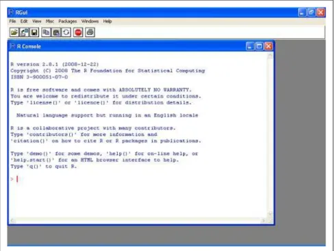
By default, R is installed into %ProgramFiles%R (which is usually C:\Program Files \R) and installed into the Start menu under the group R. When you launch R in Windows, you’ll see something like the user interface shown in Figure 2-1. Inside the R GUI window, there is a menu bar, a toolbar, and the R console.
Figure 2-1. R user interface on Windows XP
Mac OS X
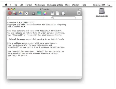
The default R installer will add an application called R to your Applications folder that you can run like any other application on your Mac. When you launch the R application on Mac OS X systems, you’ll see something like the screen shown in Figure 2-2. Like the Windows system, there is a menu bar, a toolbar with common functions, and an R console window.
On a Mac OS system, you can also run R from the terminal without using the GUI. To do this, first open a terminal window. (The terminal program is located in the Utilities folder inside the Applications folder.) Then enter the command “R” on the command line to start R.
Linux and Unix
Notice that it’s a capital “R”; filenames on Linux are case sensitive.
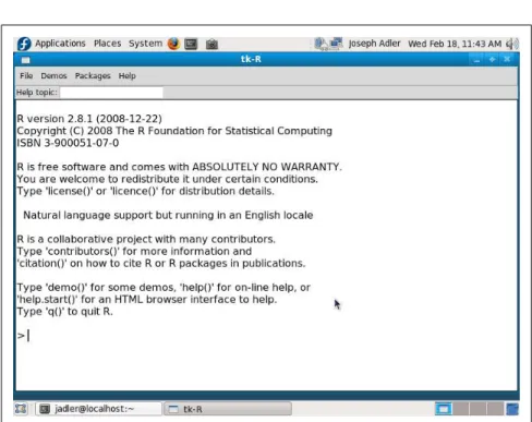
Unlike the default applications for Mac OS and Windows, this will start an inter-active R session on the command line itself. If you prefer, you can launch R in an application window similar to the user interface on other platforms. To do this, use the following command:
R -g Tk &
This will launch R in the background running in its own window, as shown in Figure 2-3. Like the other platforms, there is a menu bar with some common func-tion, but unlike the other platforms, there is no toolbar. The main window acts as the R console.
Additional R GUIs
If you’re a typical desktop computer user, you might find it surprising to discover how little functionality is implemented in the standard R GUI. The standard R GUI only implements very rudimentary functionality through menus: reading help, managing multiple graphics windows, editing some source and data files, and some other basic functionality. There are no menu items, buttons, or palettes for loading data, transforming data, plotting data, building models, or doing any interesting work with data. Commercial applications like SAS, SPSS, and S-PLUS include UIs with much more functionality.
Figure 2-2. R user interface on Mac OS X
The R Graphical User Interface | 9
Several projects are aiming to build an easier to use GUI for R:
Rcmdr
The Rcmdr project is an R package that provides an alternative GUI for R. You can install it as an R package. It provides some buttons for loading data, and menu items for many common R functions.
Rkward
Rkward is a slick GUI frontend for R. It provides a palette and menu-driven UI for analysis, data editing tools, and an IDE for R code development. It’s still a young project, and currently works best on Linux platforms (though Windows builds are available). It is available from http://sourceforge.net/apps/ mediawiki/rkward/.
R Productivity Environment
Revolution Computing recently introduced a new IDE called the R Produc-tivity Environment. This IDE provides many features for analyzing data: a script editor, object browser, visual debugger, and more. The R Productivity Environment is currently available only for Windows, as part of REvolution R Enterprise.
You can find a list of additional projects at http://www.sciviews.org/_rgui/. This book does not cover any of these projects in detail. However, you should still be able to use this book as a reference for all of these packages because they all use (and expose) R functions.
The R Console
The R console is the most important tool for using R. The R console is a tool that allows you to type commands into R and see how the R system responds. The com-mands that you type into the console are called expressions. A part of the R system called the interpreter will read the expressions and respond with a result or an error message. Sometimes, you can also enter an expression into R through the menus. If you’ve used a command line before (for example, the cmd.exe program on Win-dows) or a language with an interactive interpreter such as LISP, this should look familiar.* If not: don’t worry. Command-line interfaces aren’t as scary as they look.
R provides a few tools to save you extra typing, to help you find the tools you’re looking for, and to spot common mistakes. Besides, you have a whole reference book on R that will help you figure out how to do what you want.
Personally, I think that a command-line interface is the best way to analyze data. After I finish working on a problem, I want a record of every step that I took. (I want to know how I loaded the data, if I took a random sample, how I took the sample, whether I created any new variables, what parameters I used in my models, etc.) A command-line interface makes it very easy to keep a record of everything I do and then re-create it later if I need to.
When you launch R, you will see a window with the R console. Inside the console, you will see a message like this:
R version 2.9.2 (2009-08-24)
Copyright (C) 2009 The R Foundation for Statistical Computing ISBN 3-900051-07-0
R is free software and comes with ABSOLUTELY NO WARRANTY. You are welcome to redistribute it under certain conditions. Type 'license()' or 'licence()' for distribution details.
Natural language support but running in an English locale
R is a collaborative project with many contributors. Type 'contributors()' for more information and
'citation()' on how to cite R or R packages in publications.
Type 'demo()' for some demos, 'help()' for on-line help, or 'help.start()' for an HTML browser interface to help. Type 'q()' to quit R.
[R.app GUI 1.29 (5464) i386-apple-darwin8.11.1]
[Workspace restored from /Users/josephadler/.RData]
>
* Incidentally, R has quite a bit in common with LISP: both languages allow you to compute expressions on the language itself, both languages use similar internal structures to hold data, and both languages use lots of parentheses.
The R Console | 11
This window displays some basic information about R: the version of R you’re run-ning, some license information, quick reminders about how to get help, and a com-mand prompt.
By default, R will display a greater-than sign (“>”) in the console (at the beginning of a line, when nothing else is shown) when R is waiting for you to enter a command into the console. R is prompting you to type something, so this is called a prompt. This book includes many examples of expressions that I entered into R (and that you can enter into R) and the responses from the R system. In each of these cases, I have shown the prompt from R as a way to differentiate between the commands I entered into R and the responses from the R system.
What this means is that you should not type a command prompt (“>”) if you see one at the beginning of a line. If you want to duplicate my results, type whatever appears after the prompt. For example, I might include a snippet that looks like this:
> 17 + 3 [1] 20
This means:
• I entered “17 + 3” into the R command prompt.
• The computer responded by writing “[1] 20” (I’ll explain what that means in Chapter 3).
If you would like to try this yourself, then type “17 + 3” at the command prompt and press the Enter key. You should see a response like the one shown above. Sometimes, an R command doesn’t fit on a single line. If you enter an incomplete command on one line, the R prompt will change to a plus sign (“+”). Here’s a simple example:
> 1 * 2 * 3 * 4 * 5 * + 6 * 7 * 8 * 9 * 10 [1] 3628800
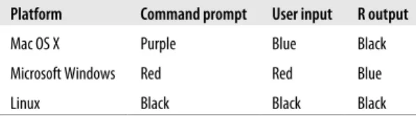
This could cause confusion in some cases (such as in long expressions that contain sums or inequalities). On most platforms, command prompts, user-entered text, and R responses are displayed in different colors to help clarify the differences. Table 2-1 presents a summary of the default colors.
Table 2-1. Text colors in R interactive mode
Platform Command prompt User input R output
Mac OS X Purple Blue Black
Microsoft Windows Red Red Blue
Command-Line Editing
On most platforms, R provides tools for looking through previous commands.† You
will probably find the most important line edit commands are the up and down arrow keys. By placing the cursor at the end of the line, you can scroll through previous commands by pressing the up arrow or the down arrow. The up arrow lets you look at earlier commands, and the down arrow lets you look at later commands. If you would like to repeat a previous command with a minor change (such as a different parameter), or if you need to correct a mistake (such as a missing paren-thesis), you can do this easily.
You can also type history() to get a list of previously typed commands.‡
R also includes automatic completions for function names and filenames. Type the “tab” key to see a list of possible completions for a function or filenames.
Batch Mode
R’s interactive mode is convenient for most ad hoc analyses, but typing in every command can be inconvenient for some tasks. Suppose that you wanted to do the same thing with R multiple times. (For example, you may want to load data from an experiment, transform it, generate three plots as Portable Document Format [PDF] files, and then quit.) R provides a way to run a large set of commands in sequence and save the results to a file. This is called batch mode.
One way to run R in batch mode is from the system command line (not the R con-sole). By running R from the system command line, it’s possible to run a set of commands without starting R. This makes it easier to automate analyses, as you can change a couple of variables and rerun an analysis. For example, to load a set of commands from the file generate_graphs.R, you would use a command like this:
% R CMD BATCH generate_graphs.R
R would run the commands in the input file generate_graphs.R, generating an output file called generate_graphs.Rout with the results. You can also specify the name of the output file. For example, to put the output in a file labeled with today’s date (on a Mac or Unix system), you could use a command like this:
% R CMD BATCH generate_graphs.R generate_graphs_`date "+%y%m%d"`.log
If you’re generating graphics in batch mode, remember to specify the output device and filenames. For more information about running R from the command line, in-cluding a list of the available options, run R from the command line with the --help option:
% R --help
† On Linux and Mac OS X systems, the command line uses the GNU readline library and includes a large set of editing commands. On Windows platforms, a smaller number of editing commands are available.
‡ As of this writing, the history command does not work completely correctly on Mac OS X. The
history command will display the last saved history, not the history for the current session.
Batch Mode | 13
You can also run commands in batch mode from inside R. To do this, you can use the source command; see the help file for source for more information.
Using R Inside Microsoft Excel
If you’re familiar with Microsoft Excel, or if you work with a lot of data files in Excel format, you might want to run R directly from inside Excel. The RExcel software lets you do just that (on Microsoft Windows systems). You can find information about this software at http://rcom.univie.ac.at/. This site also includes a single in-staller that will install R plus all the other software you need to use RExcel. If you already have R installed, you can install RExcel as a package from CRAN. The following set of commands will download RExcel, configure the RCOM server, in-stall RDCOM, and launch the RExcel inin-staller:
> install.packages("RExcelInstaller", "rcom", "rsproxy") > # configure rcom
> library(rcom) > comRegisterRegistry() > library(RExcelInstaller)
> # excecute the following command in R to start the installer for RDCOM > installstatconnDCOM()
> # excecute the following command in R to start the installer for REXCEL > installRExcel()
Follow the prompts within the installer to install RExcel.
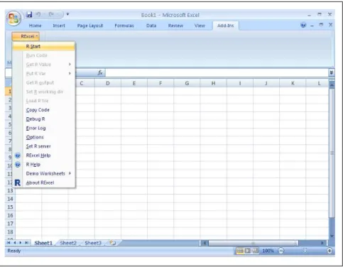
After you have installed RExcel, you will be able to access RExcel from a menu item. If you are using Excel 2007, you will need to select the “Add-Ins” ribbon to find this menu as shown in Figure 2-4. To use RExcel, first select the R Start menu item. As a simple test, try doing the following:
1. Enter a set of numeric values into a column in Excel (for example, B1:B5). 2. Select the values you entered.
3. On the RExcel menu, go to the item “Put R Var” > “Array.”
4. A dialog box will open, asking you to name the object that you are creating in Excel. Enter “v” and press the Enter key. This will create an array (in this case, just a vector) in R with the values that you entered with the name v.
5. Now, select a blank cell in Excel.
6. On the RExcel menu, go to the item “Get R Value” > “Array.”
7. A dialog box will open, prompting you to enter an R expression. As an example, try entering (v - mean(v)) / sd(v). This will rescale the contents of v, changing the mean to 0 and the standard deviation to 1.
Figure 2-4. Accessing RExcel in Microsoft Excel 2007
For some more interesting examples of how to use RExcel, take a look at the Demo Worksheets under this menu. You can use Excel functions to evaluate R expressions, use R expressions in macros, and even plot R graphics within Excel.
Other Ways to Run R
There are several open source projects that allow you to combine R with other applications:
As a web application
The Rapache software allows you to incorporate analyses from R into a web application. (For example, you might want to build a server that shows sophis-ticated reports using R lattice graphics.) For information about this project, see http://biostat.mc.vanderbilt.edu/rapache/.
As a server
The Rserve software allows you to access R from within other applications. For example, you can produce a Java program that uses R to perform some calcu-lations. As the name implies, Rserve is implemented as a network server, so a single Rserve instance can handle calculations from multiple users on different machines. One way to use Rserve is to install it on a heavy-duty server with lots of CPU power and memory, so that users can perform calculations that they couldn’t easily perform on their own desktops. For more about this project, see http://www.rforge.net/Rserve/index.html.
Other Ways to Run R | 15
Inside Emacs
3
A Short R Tutorial
This chapter contains a short tutorial of R with a lot of examples.
If you’ve never used R before, this is a great time to start it up and try playing with it. There’s no better way to learn something than by trying it yourself. You can follow along by typing in the same text that’s shown in the book. Or, try changing it a little bit to see what happens. (For example, if the sample code says 3 + 4, try typing 3 -4 instead.)
If you’ve never used an interactive language before, take a look at Chapter 2 before you start. That chapter contains an overview of the R environment, including the console. Otherwise, you might find the presentation of the examples—and the termi-nology—confusing.
Basic Operations in R
Let’s get started using R. When you enter an expression into the R console and press the Enter key, R will evaluate that expression and display the results (if there are any). If the statement results in a value, R will print that value. For example, you can use R to do simple math:
> 1 + 2 + 3 [1] 6 > 1 + 2 * 3 [1] 7 > (1 + 2) * 3 [1] 9
The interactive R interpreter will automatically print an object returned by an ex-pression entered into the R console. Notice the funny “[1]” that accompanies each returned value. In R, any number that you enter in the console is interpreted as a vector. A vector is an ordered collection of numbers. The “[1]” means that the index
of the first item displayed in the row is 1. In each of these cases, there is also only one element in the vector.
You can construct longer vectors using the c(...) function. (c stands for “com-bine.”) For example:
> c(0, 1, 1, 2, 3, 5, 8) [1] 0 1 1 2 3 5 8
is a vector that contains the first seven elements of the Fibonacci sequence. As an example of a vector that spans multiple lines, let’s use the sequence operator to produce a vector with every integer between 1 and 50:
> 1:50
[1] 1 2 3 4 5 6 7 8 9 10 11 12 13 14 15 16 17 18 19 20 21 22 [23] 23 24 25 26 27 28 29 30 31 32 33 34 35 36 37 38 39 40 41 42 43 44 [45] 45 46 47 48 49 50
Notice the numbers in the brackets on the lefthand side of the results. These indicate the index of the first element shown in each row.
When you perform an operation on two vectors, R will match the elements of the two vectors pairwise and return a vector. For example:
> c(1, 2, 3, 4) + c(10, 20, 30, 40) [1] 11 22 33 44
> c(1, 2, 3, 4) * c(10, 20, 30, 40) [1] 10 40 90 160
> c(1, 2, 3, 4) - c(1, 1, 1, 1) [1] 0 1 2 3
If the two vectors aren’t the same size, R will repeat the smaller sequence multiple times:
> c(1, 2, 3, 4) + 1 [1] 2 3 4 5
> 1 / c(1, 2, 3, 4, 5)
[1] 1.0000000 0.5000000 0.3333333 0.2500000 0.2000000 > c(1, 2, 3, 4) + c(10, 100)
[1] 11 102 13 104
> c(1, 2, 3, 4, 5) + c(10, 100) [1] 11 102 13 104 15 Warning message:
In c(1, 2, 3, 4, 5) + c(10, 100) :
longer object length is not a multiple of shorter object length
Note the warning if the second sequence isn’t a multiple of the first. In R, you can also enter expressions with characters:
> "Hello world." [1] "Hello world."
This is called a character vector in R. This example is actually a character vector of length 1. Here is an example of a character vector of length 2:
(In other languages, like C, “character” refers to a single character, and an ordered set of characters is called a string. A string in C is equivalent to a character value in R.) You can add comments to R code. Anything after a pound sign (“#”) on a line is ignored:
> # Here is an example of a comment at the beginning of a line > 1 + 2 + # and here is an example in the middle
+ 3 [1] 6
Functions
In R, the operations that do all of the work are called functions. We’ve already used a few functions above (you can’t do anything interesting in R without them). Func-tions are just like what you remember from math class. Most funcFunc-tions are in the following form:
f(argument1, argument2, ...)
Where f is the name of the function, and argument1, argument2, . . . are the arguments to the function. Here are a few more examples:
> exp(1) [1] 2.718282 > cos(3.141593) [1] -1
> log2(1) [1] 0
In each of these examples, the functions only took one argument. Many functions require more than one argument. You can specify the arguments by name:
> log(x=64, base=4) [1] 3
Or, if you give the arguments in the default order, you can omit the names: > log(64,4)
[1] 3
Not all functions are of the form f(...). Some of them are in the form of opera-tors.* For example, we used the addition operator (“+”) above. Here are a few
ex-amples of operators: > 17 + 2 [1] 19 > 2 ^ 10 [1] 1024 > 3 == 4 [1] FALSE
* When you enter a binary or unary operator into R, the R interpreter will actually translate the operator into a function; there is a function equivalent for each operator. We’ll talk about this more in Chapter 5.
Functions | 19
We’ve seen the first one already: it’s just addition. The second operator is the ex-ponentiation operator, which is interesting because it’s not a commutative operator. The third operator is the equality operator. (Notice that the result returned is FALSE; R has a Boolean data type.)
Variables
Like most other languages, R lets you assign values to variables and refer to them by name. In R, the assignment operator is <-. Usually, this is pronounced as “gets.” For example, the statement:
x <- 1
is usually read as “x gets 1.” (If you’ve ever done any work with theoretical computer science, you’ll probably like this notation: it looks just like algorithm pseudocode.) After you assign a value to a variable, the R interpreter will substitute that value in place of the variable name when it evaluates an expression. Here’s a simple example:
> x <- 1 > y <- 2 > z <- c(x,y)
> # evaluate z to see what's stored as z > z
[1] 1 2
Notice that the substitution is done at the time that the value is assigned to z, not at the time that z is evaluated. Suppose that you were to type in the preceding three expressions and then change the value of y. The value of z would not change:
> y <- 4 > z [1] 1 2
I’ll talk more about the subtleties of variables and how they’re evaluated in Chap-ter 8.
R provides several different ways to refer to a member (or set of members) of a vector. You can refer to elements by location in a vector:
> b <- c(1,2,3,4,5,6,7,8,9,10,11,12) > b
[1] 1 2 3 4 5 6 7 8 9 10 11 12 > # let's fetch the 7th item in vector b > b[7]
[1] 7
> # fetch items 1 through 6 > b[1:6]
[1] 1 2 3 4 5 6
> # fetch only members of b that are congruent to zero (mod 3) > # (in non-math speak, members that are multiples of 3) > b[b %% 3 == 0]
[1] 3 6 9 12
> # fetch items 1 through 6 > b[1:6]
[1] 1 2 3 4 5 6 > # fetch 1, 6, 11 > b[c(1,6,11)] [1] 1 6 11
You can fetch items out of order. Items are returned in the order that they are referenced:
> b[c(8,4,9)] [1] 8 4 9
You can also specify which items to fetch through a logical vector. As an example, let’s fetch only multiples of 3 (by selecting items that are congruent to 0 mod 3):
> b %% 3 == 0
[1] FALSE FALSE TRUE FALSE FALSE TRUE FALSE FALSE TRUE FALSE FALSE [12] TRUE
> b[b %% 3 == 0] [1] 3 6 9 12
In R, there are two additional operators that can be used for assigning values to symbols. First, you can use a single equals sign (“=”) for assignment.† This operator
assigns the symbol on the left to the object on the right. In many other languages, all assignment statements use equals signs. If you are more comfortable with this notation, you are free to use it. However, I will be using only the <- assignment operator in this book because I think it is easier to read. Whichever notation you prefer, be careful because the = operator does not mean “equals.” For that, you need to use the == operator:
> one <- 1 > two <- 2
> # This means: assign the value of "two" to the variable "one" > one = two
> one [1] 2 > two [1] 2
> # let's start again > one <- 1
> two <- 2
> # This means: does the value of "one" equal the value of "two" > one == two
[1] FALSE
In R, you can also assign an object on the left to a symbol on the right: > 3 -> three
> three [1] 3
† Note that you cannot use the <- operator when passing arguments to a function; you need to map values to argument names using the “=” symbol. Using the <- operator in a function will assign the value to the variable in the current environment and then pass the value returned to the function. This might be what you want, but it probably isn’t.
Variables | 21
In some programming contexts, this notation might help you write clearer code. (It may also be convenient if you type in a long expression and then realize that you have forgotten to assign the result to a symbol.)
A function in R is just another object that is assigned to a symbol. You can define your own functions in R, assign them a name, and then call them just like the built-in functions:
> f <- function(x,y) {c(x+1, y+1)} > f(1,2)
[1] 2 3
This leads to a very useful trick. You can often type the name of a function to see the code for it. Here’s an example:
> f
function(x,y) {c(x+1, y+1)}
Introduction to Data Structures
In R, you can construct more complicated data structures than just vectors. An array is a multidimensional vector. Vectors and arrays are stored the same way in-ternally, but an array may be displayed differently and accessed differently. An array object is just a vector that’s associated with a dimension attribute. Here’s a simple example.
First, let’s define an array explicitly:
> a <- array(c(1,2,3,4,5,6,7,8,9,10,11,12),dim=c(3,4))
Here is what the array looks like: > a
[,1] [,2] [,3] [,4] [1,] 1 4 7 10 [2,] 2 5 8 11 [3,] 3 6 9 12
And here is how you reference one cell: > a[2,2]
[1] 5
Now, let’s define a vector with the same contents: > v <- c(1,2,3,4,5,6,7,8,9,10,11,12)
> v
[1] 1 2 3 4 5 6 7 8 9 10 11 12
A matrix is just a two-dimensional array:
> m <- matrix(data=c(1,2,3,4,5,6,7,8,9,10,11,12),nrow=3,ncol=4) > m
Arrays can have more than two dimensions. For example:
> w <- array(c(1,2,3,4,5,6,7,8,9,10,11,12,13,14,15,16,17,18),dim=c(3,3,2)) > w
, , 1
[,1] [,2] [,3] [1,] 1 4 7 [2,] 2 5 8 [3,] 3 6 9
, , 2
[,1] [,2] [,3] [1,] 10 13 16 [2,] 11 14 17 [3,] 12 15 18
> w[1,1,1] [1] 1
R uses very clean syntax for referring to part of an array. You specify separate indices for each dimension, separated by commas:
> a[1,2] [1] 4 > a[1:2,1:2] [,1] [,2] [1,] 1 4 [2,] 2 5
To get all rows (or columns) from a dimension, simply omit the indices: > # first row only
> a[1,] [1] 1 4 7 10 > # first column only > a[,1]
[1] 1 2 3
> # you can also refer to a range of rows > a[1:2,]
[,1] [,2] [,3] [,4] [1,] 1 4 7 10 [2,] 2 5 8 11
> # you can even refer to a noncontiguous set of rows > a[c(1,3),]
[,1] [,2] [,3] [,4] [1,] 1 4 7 10 [2,] 3 6 9 12
In all the examples above, we’ve just looked at data structures based on a single underlying data type. In R, it’s possible to construct more complicated structures with multiple data types. R has a built-in data type for mixing objects of different types, called lists. Lists in R are subtly different from lists in many other languages. Lists in R may contain a heterogeneous selection of objects. You can name each component in a list. Items in a list may be referred to by either location or name.
Introduction to Data Structures | 23
Here is an example of a list with two named components: > # a list containing a number and string
> e <- list(thing="hat", size="8.25") > e
$thing [1] "hat"
$size [1] "8.25"
You may access an item in the list in multiple ways: > e$thing
[1] "hat" > e[1] $thing
[1] "hat" > e[[1]] [1] "hat"
A list can even contain other lists:
> g <- list("this list references another list", e) > g
[[1]]
[1] "this list references another list"
[[2]] [[2]]$thing [1] "hat"
[[2]]$size [1] "8.25"
A data frame is a list that contains multiple named vectors that are the same length. A data frame is a lot like a spreadsheet or a database table. Data frames are partic-ularly good for representing experimental data. As an example, I’m going to use some baseball data. Let’s construct a data frame with the win/loss results in the National League (NL) East in 2008:
> teams <- c("PHI","NYM","FLA","ATL","WSN") > w <- c(92, 89, 94, 72, 59)
> l <- c(70, 73, 77, 90, 102) > nleast <- data.frame(teams,w,l) > nleast
teams w l 1 PHI 92 70 2 NYM 89 73 3 FLA 94 77 4 ATL 72 90 5 WSN 59 102
> nleast$w [1] 92 89 94 72 59
Here’s one way to find a specific value in a data frame. Suppose that you wanted to find the number of losses by the Florida Marlins (FLA). One way to select a member of an array is by using a vector of Boolean values to specify which item to return from a list. You can calculate an appropriate vector like this:
> nleast$teams=="FLA"
[1] FALSE FALSE TRUE FALSE FALSE
Then you can use this vector to refer to the right element in the losses vector: > nleast$l[nleast$teams=="FLA"]
[1] 77
You can import data into R from another file or from a database. See Chapter 12 for more information on how to do this.
In addition to lists, R has other types of data structures for holding a heterogeneous collection of objects, including formal class definitions through S4 objects.
Objects and Classes
R is an object-oriented language. Every object in R has a type. Additionally, every object in R is a member of a class. We have already encountered several different classes: character vectors, numeric vectors, data frames, lists, and arrays.
You can use the class function to determine the class of an object. For example: > class(teams)
[1] "character" > class(w) [1] "numeric" > class(nleast) [1] "data.frame" > class(class) [1] "function"
Notice the last example: a function is an object in R with the class function. Some functions are associated with a specific class. These are called methods. (Not all functions are tied closely to a particular class; the class system in R is much less formal than that in a language like Java.)
In R, methods for different classes can share the same name. These are called generic functions. Generic functions serve two purposes. First, they make it easy to guess the right function name for an unfamiliar class. Second, generic functions make it possible to use the same code for objects of different types.
For example, + is a generic function for adding objects. You can add numbers to-gether with the + operator:
> 17 + 6 [1] 23
Objects and Classes | 25
You might guess that the addition operator would work similarly with other types of objects. For example, you can also use the + operator with a date object and a number:
> as.Date("2009-09-08") + 7 [1] "2009-09-15"
By the way, the R interpreter calls the generic function print on any object returned on the R console. Suppose that you define x as:
> x <- 1 + 2 + 3 + 4
When you type: > x [1] 10
the interpreter actually calls the function print(x) to print the results. This means that if you define a new class, you can define a print method to specify how objects from that new class are printed on the console. Some functions take advantage of this functionality to do other things when you enter an expression on the console.‡
I’ll talk about objects in more depth in Chapter 7, and classes in Chapter 10.
Models and Formulas
To statisticians, a model is a concise way to describe a set of data, usually with a mathematical formula. Sometimes, the goal is to build a predictive model with training data to predict values based on other data. Other times, the goal is to build a descriptive model that helps you understand the data better.
R has a special notation for describing relationships between variables. Suppose that you are assuming a linear model for a variable y, predicted from the variables x1, x2, ..., xn. (Statisticians usually refer to y as the dependent variable, and x1, x2, ..., xn as the independent variables.) In equation form, this implies a relationship like:
In R, you would write the relationship as y ~ x1 + x2 + ... + xn, which is a formula object.
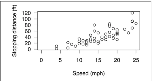
So, let’s try to use a linear regression to estimate the relationship. The formula is dist~speed. We’ll use the lm function to estimate the parameters of a linear model. The lm function returns an object of class lm, which we will assign to a variable called cars.lm:
> cars.lm <- lm(formula=dist~speed,data=cars)
Now, let’s take a quick look at the results returned: > cars.lm
Call:
lm(formula = dist ~ speed, data = cars)
Coefficients:
(Intercept) speed -17.579 3.932
As you can see, printing an lm object shows you the original function call (and thus the data set and formula) and the estimated coefficients. For some more information, we can use the summary function:
> summary(cars.lm)
Call:
lm(formula = dist ~ speed, data = cars)
Residuals:
Min 1Q Median 3Q Max -29.069 -9.525 -2.272 9.215 43.201
Coefficients:
Estimate Std. Error t value Pr(>|t|) (Intercept) -17.5791 6.7584 -2.601 0.0123 * speed 3.9324 0.4155 9.464 1.49e-12 ***
---Signif. codes: 0 ‘***’ 0.001 ‘**’ 0.01 ‘*’ 0.05 ‘.’ 0.1 ‘ ’ 1
Residual standard error: 15.38 on 48 degrees of freedom Multiple R-squared: 0.6511, Adjusted R-squared: 0.6438 F-statistic: 89.57 on 1 and 48 DF, p-value: 1.490e-12
As you can see, the summary option shows you the function call, the distribution of the residuals from the fit, the coefficients, and information about the fit. By the way, it is possible to simply call the lm function or to call summary(lm(...)) and not assign a name to the model object:
> lm(dist~speed,data=cars)
Call:
lm(formula = dist ~ speed, data = cars)
Coefficients:
(Intercept) speed -17.579 3.932
> summary(lm(dist~speed,data=cars))
Call:
lm(formula = dist ~ speed, data = cars)
Residuals:
Min 1Q Median 3Q Max
Models and Formulas | 27