Cubic-spline interpolation to estimate effects of inbreeding on milk yield in first lactation Holstein cows

Cubic-spline interpolation to estimate effects of inbreeding

on milk yield in first lactation Holstein cows

Makram J. Geha

, Jeffrey F. Keown

and L. Dale Van Vleck

Department of Animal Science, University of Nebraska, Lincoln, NE, USA.

2

_{Roman L. Hruska U.S. Meat Animal Research Center, ARS, USDA, Lincoln, NE, USA.}

Abstract

Milk yield records (305d, 2X, actual milk yield) of 123,639 registered first lactation Holstein cows were used to com-pare linear regression (y =b0+b1X + e) ,quadratic regression, (y =b0+b1X +b2X

2

+e) cubic regression (y =b0+b1X +

b2X 2

+b3X 3

+e) and fixed factor models, with cubic-spline interpolation models, for estimating the effects of inbreed-ing on milk yield. Ten animal models, all with herd-year-season of calvinbreed-ing as fixed effect, were compared usinbreed-ing the Akaike corrected-Information Criterion (AICc). The cubic-spline interpolation model with seven knots had the lowest AICc, whereas for all those labeled as “traditional”, AICc was higher than the best model. Results from fitting inbreed-ing usinbreed-ing a cubic-spline with seven knots were compared to results from fittinbreed-ing inbreedinbreed-ing as a linear covariate or as a fixed factor with seven levels. Estimates of inbreeding effects were not significantly different between the cu-bic-spline model and the fixed factor model, but were significantly different from the linear regression model. Milk yield decreased significantly at inbreeding levels greater than 9%. Variance component estimates were similar for the three models. Ranking of the top 100 sires with daughter records remained unaffected by the model used.

Key words:Akaike's information criterion, cubic-spline interpolation, inbreeding, milk yield. Received: April 23, 2010; Accepted: February 28, 2011.

Introduction

Commercial adoption of artificial insemination by the dairy industry has facilitated the intensification of selection for traits such as milk, fat and protein yields. Selection is largely based on Predicted Transmitting Ability (PTA), re-sulting from best linear unbiased prediction (BLUP) and se-lection indices. Both the moderate heritability of production traits and the use of BLUP have lead to the predominant use of specific family-lines of bulls (Weigel, 2001), especially in the Holstein population, which in turn has resulted in mating of related animals. A consequence of such matings is an in-crease in average inbreeding. The development of multiple ovulation and embryo transfer technology have also contrib-uted to increasing levels of inbreeding by intensifying selec-tion for high producing cows used as dams of AI bulls (Kearneyet al., 2004). The average inbreeding coefficient in the Holstein population in the United States, as reported by the Animal Improvement Program Laboratory for animals born between January and June of 2009 (using 1960 as base year), was 5.50% (ARS-AIPL, 2009). Several studies have shown the detrimental effects of inbreeding on several pro-duction, reproduction and health traits, even at low levels. For example, Hudson and Van Vleck (1984a,b) studied

ef-fects of inbreeding on first lactation milk and fat production in five dairy breeds, using a linear regression approach. They reported decreased milk yield in inbred animals in all the five breeds, with an estimated loss of 21 kg of milk per 1% in-crease in the inbreeding coefficient in Holsteins. They also noted that the effects of inbreeding were non-linear, when in-breeding was modelled as a classification variable. With similar statistical models, Miglioret al. (1992) reported a significant reduction in total milk yield of 10 kg for each 1% increase in inbreeding in Canadian Jersey cattle. The Cana-dian group also reported the non-linear effects of inbreeding. Thompsonet al.(2000) found a decrease in milk yield of 35 kg per 1% increase in inbreeding between 0 and 7%, com-pared to a 55 kg per 1% increase for higher levels of inbreed-ing in Holstein cows, this again indicatinbreed-ing a non-linear effect on milk yield.

The most common method used to estimate effects of inbreeding is linear regression of production on inbreeding coefficient (e.g., Falconer and MacKay, 1996). The regres-sion coefficient is the expected change in the trait of interest per 1% increase in inbreeding and is a measure of inbreeding effects. Few studies have used non-linear regression of pro-duction on inbreeding coefficient. McParlandet al.(2007), when comparing models with higher order polynomials and a classification model, reported significant quadratic effects when considering inbreeding as either a continuous variable www.sbg.org.br

Send correspondence to Makram J. Geha. Department of Animal Science, University of Nebraska, Lincoln, NE 68583-0908, USA. E-mail: mjgeha@huskers.unl.edu.

or a fixed factor. Nevertheless, they urged caution in inter-preting nonlinear results, due to large-standard errors in esti-mates at higher levels of inbreeding. Croquetet al.(2007) compared the fit of linear (y=b0+b1X+e), quadratic (y=b0

+b1X+b2X2+e) and cubic (y=b0+b1X+b2X2+b3X3+e)

regression models for estimating the effects of inbreeding based on milk yield. The coefficients in all the three methods were significantly different from zero. The largest t-value was for the simple linear regression coefficient. They pro-posed using the linear regression model for estimating the ef-fects of inbreeding, especially for animals less than 10% in-bred. Gulisijaet al.(2007) used a non-parametric approach to estimate inbreeding effects on production in Jerseys. They reported that, on including inbreeding as a linear covariate, the fit of the model at low levels of inbreeding improved (< 7%). The lack of fit was detected in the linear regression model at higher levels of inbreeding (> 10%), for which a third-order regression model seemed to adequately fit the data. Another method which could be used is cubic-spline in-terpolation to estimate the non-linear effects of inbreeding on milk yield. The rationale is that this method, besides pro-viding better coverage of data points (Harrell Jr, 2001), may result in more accurate estimates of the effects of inbreeding on milk yield.

The objective of this study was to compare cubic-spline interpolation to estimate effects of inbreeding on milk yield with traditional linear regression and fixed factor models.

Materials and Methods

Data and edits

Records of actual milk yield adjusted to 305-d in lac-tation (2X) for first-calf Holstein heifers, freshening between 2002 and 2006, were used. The records were pro-vided by the Dairy Herd Information Association (DHIA-North Carolina). Only records of registered Holstein heif-ers were included in the analysis. Animals with less than five recorded test-day milk yields were deleted from the data. Records of annual milk yield included in the data set, consisted of milk records within four times the standard de-viation from the average (approximately 9,100 kg). As standard deviation was approximately 1,660 kg, rounding up the confidence range to the nearest 100 kg resulted in some yields that were less than 2,400 kg, and others more than 15,800 kg. Through being considered as outliers, these were omitted from the data set. Contemporary groups were herd-year-seasons (HYS) of freshening, with season 1 de-fined as October 1 through March 31, and season 2 dede-fined as April 1 through September 30. Records of HYS with less than 10 freshening heifers were deleted. Pedigree informa-tion was provided by the Holstein Associainforma-tion, USA. The pedigree file used was extended backwards, so that at least one of the paternal and maternal grandsires or granddams was known for all the heifers included in the analysis.

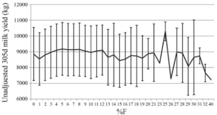
Re-cords of animals that did not fit the minimum requirements were omitted. Nonetheless, these animals were included in the pedigree file, which finally consisted of 541,249 ani-mals. Individual inbreeding coefficients (%F) were pro-vided by AIPL, as calculated by Wigganset al.(1995). Af-ter edits, the analysis included records of 123,639 heifers in 5,839 HYSs, with individual inbreeding coefficients rang-ing from 0 to 40%. Few animals (approximately 0.1%) had levels of inbreeding greater than 18.75%. The distribution of inbreeding coefficients was similar to that found in pre-vious studies (e.g., Hudson and Van Vleck, 1984a,b; Mi-glior et al., 1992). Figure 1 presents average unadjusted milk yields with values within one standard deviation) by inbreeding class. Fluctuation of averages for inbreeding co-efficients greater than 12% may be due to the small number of animals in those categories. In fact, milk yield records of animals with inbreeding greater than 12% constituted less than 1% of the available data, with several of these inbreed-ing levels (8 out of 19) havinbreed-ing less than 10 observations each.

Statistical models

All the models included a random animal genetic ef-fect with HYS treated as a fixed factor. The ten models compared were grouped as follows:

Fixed factor models

The first model was a saturated fixed-factor model, where the inbreeding coefficients (F) were included as lev-els of a fixed factor. Inbreeding coefficients rounded to the nearest integer were considered as unique levels. Thus, 32 different inbreeding levels were formed (0% to 40%, with levels 22, 24 and 33 through 39 missing).

The second fixed factor model consisted of grouping F into seven classes as shown in Table 1. This classification has been used in several studies (e.g., Hudson and Van Vleck, 1984a,b; Miglior et al., 1992; McParland et al., 2007).The general form of the fixed factor models is:

yijkl=m+Fi+HYSj+Animalk+eijkl

withyijkl, milk yield of Animalkin HYSjwith an

inbreed-ing coefficient F fallinbreed-ing within inbreedinbreed-ing leveli;m, a

stant;FI,the effect of theithlevel of inbreeding fori= 1, ...,

32 with the saturated fixed factor model, andi= 1, ..., 7 with the fixed factor model;HYSj, the effect of thejthHYS

con-temporary group treated as a fixed factor;Animalk, a

ran-dom additive genetic value of the kth animal with

sa2= 0.5se2, andeijkl, a random error effect normally and

in-dependently distributed with a mean of zero and a variance,

se2.

Regression models

Inbreeding coefficients were included as covariates with linear, linear and quadratic or linear, quadratic and cu-bic effects, resulting in three models.

The linear regression model was:

yijk=b0+b1F+HYSi+Animalj+eijk

withyijk, milk yield of Animaljin HYSiwith an inbreeding

coefficient F;b0, intercept;b1, regression coefficient for the

linear effect of inbreeding;F, inbreeding coefficient of ani-malj;HYS,Animalandeeffects as defined earlier.

The linear and quadratic regression model was:

yijk=b0+b1F+b2F2+HYSi+Animalj+eijk

withyijk, milk yield of Animaljin HYSiwith an inbreeding

coefficient F;b0, intercept;b1, coefficient of the linear

ef-fect of inbreeding;F, inbreeding coefficient of animalj;b2,

coefficient for the quadratic effect of inbreeding; andHYS, Animalandeeffects as defined earlier.

The cubic regression model was:

yijk=b0+b1F+b2F2+b3F3+HYSi+Animalj+eijk

withyijk, milk yield of Animaljin HYSiwith an inbreeding

coefficient F;b0, intercept;b1, coefficient of the linear

ef-fect of inbreeding;F, inbreeding coefficient of animalk;b2,

coefficient for the quadratic effect of inbreeding;b3,

coeffi-cient for the cubic effect of inbreeding; andHYS,Animal andeeffects as defined earlier.

Cubic-spline models

The spline models had three to seven knots (t3… t7)

for F. Choice of knots was based on consideration of the

different possible inbreeding coefficients that could be at-tained from mating of directly related animals such as full-sibs, half-sibs,parent- progeny and grandparent-grand-progeny matings. Some knots were also chosen to divide the inbreeding levels into equally spaced groups. For the cubic-spline model with seven knots, the knots were chosen to match the seven levels of the fixed factor model. The knot positions are presented in Table 2. This approach re-sulted in five different models, the most complete being:

yijk=b0+b1F+b2F2+b3F3+HYSi+Animalj+eijk

withyijk, milk yield of Animaljin HYSiwith an inbreeding

coefficient F;b0, intercept;b1, coefficient for the linear

ef-fect of inbreeding; F, inbreeding coefficient of animalj;

b1, ...,b6, the Z-spline coefficients of the cubic-spline

inter-polation for F;F2, ...,F6, the knot functions; andHYS, Ani-malandeeffects as previously described.

Depending on the number of knots in the model, some terms were removed.

Other models could have also been used; for example, higher order linear polynomials, such as quartic and quin-tic. Inclusion of other fixed and /or random effects might improve the fit of the model. The focus of the project was to compare cubic-spline interpolation with traditionally used models. Thus, the models used were kept as similar as pos-sible to the traditional models. Furthermore, as discussed later, comparisons required fixed genetic variance. Animal genetic variance was chosen to match heritability estimates from other studies (e.g., Swalve and VanVleck, 1987).

All analyses were conducted using ASREML 2.0 (Gilmouret al., 2006).

Model comparisons

Models were compared using Akaike's Information Criterion (AIC; Akaike, 1974), one of the several model se-lection methods based on the principle of parsimony. Other methods based on the same principle could have been used but the AIC is one of the easiest methods to compute and does not require extensive computation. Model selection could have been also conducted in the context of null hy-pothesis testing, however this approach has relatively poor performance given its dependence on the significance level specified to test if effects should be included or omitted

Table 1- Classification of inbreeding into seven levels, and the number of cows per category.

Inbreeding levels Numberof cows

0% 794

0-3.125% 16308

3.125-6.250% 81805

6.250-12.500% 23832

12.500-18.750% 780

18.750-25.000% 36

> 25.000% 84

Table 2- Position of knots at inbreeding levels (%F) for the five cu-bic-spline models.

Number of knots Position of knots

3 0, 12.500, 25.000

4 0, 6.250, 12.500, 25.000

5 0, 3.125, 6.250, 12.500, 25.000

6 0, 3.125, 6.250, 12.50, 18.750, 25.000

from a model (a= 0.05 or 0.01 or 0.15). The null hypothe-sis testing approach also has a relatively poor performance when testing non-nested models (Burnham and Anderson, 2002). The AIC is an approximate measure of the Kullback-Leibler information of a model based on the mate of log-likelihood and number of parameters esti-mated:AIC= 2p- 2l, wherepis the number of parameters estimated, andl is the log-likelihood of the model used. When the ratio of the number of observations,n, to the number of parameters estimated,p, is less than 40, it is rec-ommended that corrected AIC be used: AICc = AIC + [2p(p + 1)/(n - p- 1)] (Burnham and Anderson, 2002). As the number of observations becomes large, AICc converges to AIC. The idea behind AIC is that the difference between two competing models, A and B, can be detected by differ-ences in estimates of residual error variances from the two models. As, by increasing the number of parameters in a model, the goodness of fit improves,i.e., there is a reduc-tion in the residual sum of squares and an increase in log-likelihood in nested models, a growing penalty func-tion, equal to twice the number of parameters included, is deducted to discourage “overfitting”. One disadvantage of overfitting is that, given enough parameters, an irrational model may fit the data perfectly, even if it does include nonsensical parameters. Models were ranked according to their AICc because the ratio of the number of observations to the number of parameters estimated, was always less than 40. The model with the smallest AICc was considered the best. The significance of differences between models was based on their AICc values, as described by Burnham and Anderson (2002) for comparison of models. In general, a small difference in AICc between two competing models (less than 2) indicates that neither of the two is adequate. A moderate difference (4 to 7) indicates that the model with the higher AICc does not fit the data as well as the one with the lower AICc rank. A large difference (greater than 10) indicates that the model with the highest AICc is inade-quate compared to that with the lowest. The log-likelihood used in the AIC, and subsequently the AICc, is based on maximizing likelihood (ML). The software used in the analysis however maximized the restricted maximum like-lihood (REML). Comparison of the different models there-fore required manipulation of the likelihood estimates from REML to be converted into ML estimates. Therefore, the animal genetic variance was fixed for all models to facili-tate estimating random residual variance. Heritability of milk yield at first lactation was assumed to be 0.33 (Swalve and Van Vleck, 1987; Miglioret al., 1992). The additive genetic component of variance was fixed at half resid-ual-error variance to facilitate comparing models. With ge-netic variance as a fixed function of residual-error variance,

only the residual-variance component needed to be esti-mated. The next step was to convert the REML estimate of residual-error variance into the ML estimate for computing likelihood and AIC. The method of transformation from REML to ML estimates is as follows:

The REML estimate of residual-error variance, $

seREML

2

, is equal to the sum of squares of the residuals (SSR), divided by the degrees of freedom for error (dfe), whereas

the ML estimate of residual-error variance,s$ML 2

is equal to SSR divided by the total number of observations (n). This leads to the following adjustment: s$_e / _e

REML SSR df

2 ₌ )

and

$ /

s_e

ML SSR n

2 ₌ )

, then SSR df_{e e} n _e

REML ML

)

= ´s$2 = ´s$2

so that

s_{e e} s_e

ML df n REML

2 _{= ´} 2

( / ) .

Milk yield was assumed to be approximately nor-mally distributed,y ~N(Xb, Vse2), so that the likelihood

function givenyis:

L y V

y X e e n n ( , | ) ( ) | |

exp ( )' (

/ b s ps b 2 2 2 1 2 1 2 =æ è ç ç ö ø ÷ ÷ ´ -

-Vse y Xb 2 1 ) (- - ) é ëê ù ûú

whereyis thenx1vector of observations;nis total number of observations;Vis a matrix of constants, since the animal genetic variance was fixed at one-half residual-error vari-ance;se2is the residual-error variance; andse

2

is the product

of the design matrix,X,and the vector of fixed effects,b. Thus, the log-likelihood function is:

l y n n n V

y X V

e e

( , | ) ln( ) ln( ) ln| |

( )'

b s p s

b

2 2

2 2 2 2

1 2

= - - -

-- -1

2

(y X )

e -é ë ê ù û ú b s

To find the estimate ofse2that maximizes likelihood,

the first derivative with respect tose2:

d b s

ds s

b b

s

l e y n y X V y X

e e e

( , 2| ) ( )' ( )

2 2 1 4 0 2 0 1 2

= - - + æ -

-è ç -ç ö ø ÷ ÷

is equated to zero. This permits estimatingse

2

from

n y X V y X

e e 2s b b s $ ( )' ( ) 2 1 4 1 2

= æ -

-è ç ç ö ø ÷ ÷ -and so that 1

2

(

ˆ

) '

(

ˆ

)

ML

e

y

X

V

y

X

n

b

b

s

=

-

-4

1 2

1

_ˆ

_ˆ

[(

) '

(

)]

2

2

n

y

X

V

y

X

s

b

b

s

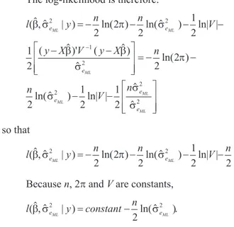
-The log-likelihood is therefore:

l y n n V

y

eML eML

($,$ | ) ln( ) ln($ ) ln| |

(

b s2 p s2

2 2 2

1 2

1 2

= - - -

--

-é

ë ê ê

ù

û ú

ú= -

-X V y X n

n

e

e

ML

M

$)' ( $)

$ ln( )

ln($

b b

s p

s

1

2 ₂ 2

2 L

ML

ML

V n e

e 2

2

2

1 2

1 2

) ln| | $

$

- - é

ë ê ê

ù

û ú ú s s

so that

l( eML y n n eML V n

$,$ | ) ln( ) ln($ ) ln| |

b s2 p s2

2 2 2

1

2 2

= - - -

-Becausen, 2pandVare constants,

l(b s$,$eML| )y nln(s$eML)

2 2

2

=constant- .

The constant is the same for all models becausen, 2p andVare the same for all models.

Comparison of models for inbreeding effects

The analyses were re-run without restrictions on the animal genetic variance to obtain, not only estimates of variance components and predicted animal breeding values for traditional linear regression and fixed factor models, but also the best cubic-spline model for comparing estimates of the effects of inbreeding on milk yield and of variance com-ponents and heritability. For each model, the predicted breeding values (EBV) for sires of daughters with records were compared to detect changes in sire-ranking due to the model used. The pedigree file contained 9,618 sires of which 1,409 had daughters with records. The proc reg pro-cedure in SAS©9.2 was used to regress EBVs of these sires from the cubic-spline model, on the corresponding EBV from the fixed factor and linear regression models. The cal-culated correlations among EBV of sires of daughters with records from all three methods were examined using the

proc corr procedure in SAS©9.2. Ranking of the top 100 sires for the three models were also compared. Finally, the estimated milk yields by inbreeding level using the best model were regressed on estimated milk yields by inbreed-ing level from the linear regression and fixed factor models using the proc reg procedure in SAS©9.2.

Results and Discussion

Estimates of residual-error variance, log-likelihood, and AICc for each model, as well as differences in AICc from the model with the lowest AICc (assumed best), are given in Table 3. Based on AICc, the best model was cu-bic-spline interpolation of inbreeding with seven knots. The model with the highest AICc was the saturated fixed factor model (a difference of +50.447 from the best model). The fixed factor model and simple linear regression model, i.e.the traditional methods of analysis, ranked second and third to last, respectively. The cubic-spline model with 4 knots had 0.48 higher AICc than the model with seven knots indicating that the two models are nearly equivalent. The cubic-spline models with five and six knots as well as the cubic regression model had AICc differences from the best model ranging between 2 and 6 reflecting that these models do not fit the data as well as the best model. The re-maining models (i.e.linear regression, linear and quadratic regression, cubic-spline with three knots, fixed factor and saturated models) all had differences of AICc larger than 10 units compared with the best model indicating a poor fit to the data compared to the cubic-spline with seven knots.

The counter-intuitive result of the cubic-spline mod-els with five and six knots, which performed worse than that with four, is explained by differences in log-like-lihoods and the number of parameters between the mod-els. Compared to the model with four knots, one additional parameter was estimated in the model with five knots, and two in that with 6. Even though this difference was small, it lead to AICc ranking differing from what was to be expected.

Table 3- Estimates of residual variance, logarithm of the likelihood and AICc for each model, with differences in AICc from the cubic-spline model with seven knots.

Model s$e

2

(kg2) (x10,000) LogL (-865,000) AICc (1,742,500) Difference in AICc

Cubic-spline with 7 knots 125.515 -122.913 15.995 0

Cubic-spline with 4 knots 125.519 -126.458 16.473 0.479

Cubic-spline with 5 knots 125.520 -126.425 18.612 2.618

Cubic-spline with 6 knots 125.521 -126.393 20.751 4.756

Linear, quadratic and cubic regression 125.524 -128.920 21.398 5.404

Linear and quadratic regression 125.532 -133.385 28.124 12.130

Cubic-spline with 3 knots 125.534 -134.370 30.094 14.100

Linear regression 125.539 -137.357 33.865 17.870

Fixed factor 7 125.546 -138.180 50.934 34.940

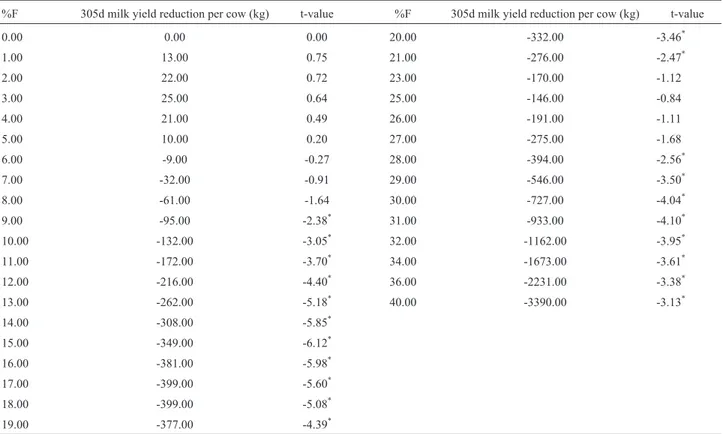
Estimates of the effects of inbreeding on milk yield for a cubic-spline model with seven knots are represented in Figure 2. Table 4 contains t-values to test for significance of reduction in 305d milk yield between each inbreeding level and no inbreeding. Significant differences at the 0.05 rejection level were at |t-value| > 1.96. These results showed no significant decrease in milk production up to an inbreeding level of 8%. Milk yields significantly decreased at inbreeding levels of 9% to 21%. No significant differ-ences in milk yields were found for inbreeding levels of 23% to 27%. Significant differences in milk yields were de-tected for inbreeding levels of 28% and beyond.

The linear regression model indicated a decrease of 21.49 kg of milk per 1% increase in inbreeding, in agree-ment with estimates in the literature for Holstein cattle, which ranged from 9.84 to 26.00 kg (Thompson et al., 2000). Estimates of losses due to inbreeding using the fixed factor model are represented in Table 5. These estimates generally agree with previous studies in which five in-breeding classes were used (Hudson and Van Vleck, 1984a,b; Miglioret al., 1992; Thompsonet al., 2000).

Estimates of variance components and heritability for the cubic-spline model with seven knots, for the linear re-gression model and for the fixed factor model with seven levels are shown in Table 6. The three models resulted in similar estimates of variance components and heritability

Figure 2- Estimated 305 d milk yields (kg) by inbreeding level (%F) from the cubic-spline model adjusted for herd-year-season effects.

Table 4- t statistics for testing significance in the reduction of 305 d milk yield (kg) between different inbreeding levels and 0% inbreeding from the cu-bic-spline interpolation model with seven knots.

%F 305d milk yield reduction per cow (kg) t-value %F 305d milk yield reduction per cow (kg) t-value

0.00 0.00 0.00 20.00 -332.00 -3.46*

1.00 13.00 0.75 21.00 -276.00 -2.47*

2.00 22.00 0.72 23.00 -170.00 -1.12

3.00 25.00 0.64 25.00 -146.00 -0.84

4.00 21.00 0.49 26.00 -191.00 -1.11

5.00 10.00 0.20 27.00 -275.00 -1.68

6.00 -9.00 -0.27 28.00 -394.00 -2.56*

7.00 -32.00 -0.91 29.00 -546.00 -3.50*

8.00 -61.00 -1.64 30.00 -727.00 -4.04*

9.00 -95.00 -2.38* 31.00 -933.00 -4.10*

10.00 -132.00 -3.05* _{32.00 -1162.00 -3.95}*

11.00 -172.00 -3.70* 34.00 -1673.00 -3.61*

12.00 -216.00 -4.40* _{36.00 -2231.00 -3.38}*

13.00 -262.00 -5.18* _{40.00 -3390.00 -3.13}*

14.00 -308.00 -5.85*

15.00 -349.00 -6.12*

16.00 -381.00 -5.98*

17.00 -399.00 -5.60*

18.00 -399.00 -5.08*

19.00 -377.00 -4.39*

*Significant reduction in milk yield from the estimated milk yield at 0% inbreeding (p < 0.05).

Table 5- Estimated annual milk yield loss (kg) at different inbreeding lev-els for the fixed factor model with seven levlev-els.

Inbreeding levels Milk yield loss (kg)

0+-3.125% 5.92±18.85

3.125+-6.25% 78.64±21.15

6.25+_-12.5%

386.10±52.45 12.5+_-18.75%

366.17±208.70

18.75+-25% 479.75±148.62

of approximately 0.31 (SD = 0.01) which agrees with esti-mates of heritability reported in the literature of 0.33 (e.g., Swalve and Van Vleck, 1987).

Regression of EBV from the cubic-spline model on EBV from the linear regression model for the 1,409 sires having daughters with records, resulted in R2 of 0.99, a correlation of 0.99 and a regression coefficient of 0.97. Regression of EBV from the cubic-spline model on EBV from the fixed factor model had a R2of 0.99, a correlation of 0.99 and a regression coefficient of 0.99. The regres-sion coefficient from regresregres-sion of EBV from the cu-bic-spline model on the EBV from the linear regression model, was significantly different from 1.00 (p < 0.0001). The regression coefficient of the regression of EBV from the cubic-spline model on the EBV from the fixed factor model, was not significantly different from 1.00 (p = 0.31). Correlations between EBV from the cubic-spline model and EBV from the linear regression and fixed factor models were both significantly different from 1.00 (p < 0.0001), when the Fisher (rho0 = 1.00) option was specified in the CORR procedure in SAS©. Thus, esti-mates of breeding values could possibly be different for the three models. Nonetheless, ranking of the top 100 sires by each method revealed that only the rank of one sire changed between the linear regression model and the two other models indicating that selection for breeding value was minimally affected by the model used.

The regression of milk yield estimates by inbreeding level from the cubic-spline model on milk yield estimates by inbreeding level from the linear regression model had a R2of 0.99, a correlation of 0.79 and a regression coefficient of 0.97 that was significantly different from 1.00 (p = 0.02). The regression of estimates by inbreeding level from the cubic-spline model on estimates by inbreeding level from the fixed factor model had a R2of 0.99, a correlation of 0.88 and a regression coefficient of 0.98 that was not signifi-cantly different from 1.00 (p = 0.13).

Consequently, the linear regression model is appar-ently not the best for estimating the effects of inbreeding on milk yield. Despite its lower AICc ranking, the fixed factor model appears to be a simpler and more effective alterna-tive to the more complex cubic-spline. Estimates of the ef-fects of inbreeding on milk production were similar for the cubic-spline model and the fixed factor model. This may be due to the positions of the knots in the cubic-spline model which coincide, for the most part, with the inbreeding lev-els for the fixed factor model.

A substantial reduction in profit is reflected from losses derived from the detrimental effects of inbreeding. At an inbreeding level of 9%, the estimated loss in milk yield would be 95 kg, thereby reflecting a potential loss of US$ 26.18 per lactation at the average milk-price of US$ 12.5 per hundred weight. The average inbreeding in the U.S. Holstein population was 5.50% for the year 2009, and is on the increase, as reported by the Animal Improve-ment Program Laboratory.

In this study, knots were positioned at inbreeding lev-els reflecting the possible mating of directly related animals (within a family line). Therefore, given the similarity in es-timates of effects of inbreeding on milk yield, the fixed fac-tor model, despite poorer AICc, presents a simple and effective alternative to using the complex cubic-spline.

If adjustment of milk yields for inbreeding is to be based on estimates using a cubic-spline model, it would be advantageous to develop an algorithm, useful in detecting the positions of knots providing the best fit to the data. Their positioning would first need to be defined in one or several reference data sets, and then validated in others. Cu-bic-spline coefficients would require periodical re-valida-tion.

Acknowledgments

This manuscript is a contribution of the University of Nebraska Agricultural Research Division, supported in part by funds provided through the Hatch Act, USDA.

The authors would like to thank the Holstein Associa-tion U.S.A for providing the pedigree file, as well as the Animal Improvement Program Laboratory of ARS-USDA for providing estimates of inbreeding coefficients on the cows used in this study. The authors also wish to express their gratitude to Dr. Stephen Kachman for guidance and assistance in model comparison.

References

Akaike H (1974) A new look at the statistical model identifica-tion. IEEE Transact Autom Control 19:716-723.

Burnham KP and Anderson DR (2002) Model Selection And Multimodel Inference, 2nd edition. Springer, New York, 353 pp.

Croquet C, Mayeres P, Gillon A, Hammami H, Soyeurt H, Van-derick S and Gengler N (2007) Linear and curvilinear effects of inbreeding on production traits for Walloon Holstein cows. J Dairy Sci 90:465-471.

Table 6- Estimates of variance components (kg/100)2and heritability for the three models.

Model sa

2 _s

p

2

Heritability

Linear regression 59.50±2.24 187.40±0.98 0.31±0.01

Fixed factor with seven levels 58.90±2.23 187.20±0.98 0.31±0.01

Falconer DS and MacKay TFC (1996) Introduction to Quantita-tive Genetics. 4th edition. Addison Wesley Longman, Har-low, 438 pp.

Gilmour AR, Gogel BJ, Cullis BR and Thompson R (2006) ASReml User Guide Release 2.0 VSN International Ltd, Hemel Hempstead.

Gulisija D, Gianola D and Weigel KA (2007) Nonparametric analysis of the impact of inbreeding on production in Jersey cows. J Dairy Sci 90:493-500.

Harrell Jr FE (2001) Regression Modeling Strategies. Springer, NewYork, 568 pp.

Hudson GFS and Van Vleck LD (1984a) Inbreeding of artificially bred dairy cattle in the Northern United States. J Dairy Sci 67:161-170.

Hudson GFS and Van Vleck LD (1984b) Effects of inbreeding on milk and fat production, stayability, and calving interval of registered Ayrshire cattle in the Northeastern United States. J Dairy Sci 67:171-179.

Kearney JF, Wall E, Villaneuva B and Coffey MP (2004) In-breeding trends and application of optimized selection in the UK Holstein population. J Dairy Sci 87:3503-3509. McParland S, Kearney F, Rath M and Berry DP (2007) Inbreeding

effects on milk production, calving performance, fertility and conformation in Irish Holstein-Friesians. J Dairy Sci 90:4411-4419.

Miglior F, Szkotnicki B and Burnside EB (1992) Analysis of lev-els of inbreeding and inbreeding depression in Jersey cattle. J Dairy Sci 75:1112-1118.

Swalve H and Van Vleck LD (1987) Estimation of genetic (Co) variances for milk yield in first three lactations using an ani-mal model and restricted maximum likelihood. J Dairy Sci 70:842-849.

Thompson JR, Everett RW and Hammerschmidt NL (2000) Ef-fects of inbreeding on production and survival in Holsteins. J Dairy Sci 83:1856-1864.

Weigel KA (2001) Controlling inbreeding in modern breeding programs. J Dairy Sci 84:E177-E184.

Wiggans GR, VanRaden PM and Zuurbier J (1995) Calculation and use of inbreeding coefficients for genetic evaluation of United States dairy cattle. J Dairy Sci 78:1584-1590.

Internet Resources

Animal Improvement Program Laboratory (ARS-AIPL) August 2009 Inbreeding information http://aipl.arsusda.gov/eval/ summary/inbrd.cfm (September 14, 2009).

Associate Editor: Alexandre Rodrigues Caetano