A QUALITATIVE REASONING APPROACH FOR IMPROVING QUERY RESULTS FOR SKETCH-BASED QUERIES BY TOPOLOGICAL ANALYSIS OF SPATIAL AGGREGATION

i

A QUALITATIVE REASONING APPROACH FOR IMPROVING QUERY RESULTS FOR

SKETCH-BASED QUERIES BY TOPOLOGICAL ANALYSIS OF SPATIAL AGGREGATION

ii

A QUALITATIVE REASONING APPROACH FOR IMPROVING QUERY RESULTS

FOR SKETCH-BASED QUERIES BY TOPOLOGICAL ANALYSIS OF SPATIAL

AGGREGATION

Dissertation supervised by

PhD Prof. Joaquin Huerta PhD Prof. Angela Schwering

PhD Prof. Marco Painho

iv

ACKNOWLEDGEMENTS

vi

A QUALITATIVE REASONING APPROACH FOR IMPROVING QUERY RESULTS

FOR SKETCH-BASED QUERIES BY TOPOLOGICAL ANALYSIS OF SPATIAL

AGGREGATION

ABSTRACT

Sketch-based spatial query systems provide an intuitive method of user interaction for

spatial databases. These systems must be capable of interpreting user sketches in a way

that matches the information that the user intended to provide. One challenge that must be

overcome is that humans always simplify the environments they have experienced and this

is reflected in the sketches they draw. One such simplification is manifested as aggregation

or combination of spatial objects into conceptually or spatially related groups.

In this thesis I develop a system that uses reasoning tools of the RCC-8 to evaluate

sketch-based queries and provide a method for minimizing the effects of aggregation by

determining whether a solution to a query can be expanded if some groups of regions are

assumed to be parts of a larger aggregate region. If such a group of regions is found, then

this group must be included in the solution. The solution is approximate because the

approach taken only verifies that assumed parts of an aggregate are not inconsistent with

the configuration of the whole solution. Only cases where the size of the solution equals the

size of the query minus one are analysed.

vii

KEYWORDS

Region Connection Calculus

Spatial Aggregation

Spatial Reasoning

Spatial Queries

viii

ACRONYMS

GIS – Geographic Information Systems

QSR – Qualitative Spatial Reasoning

QSKR – Qualitative Spatial Knowledge Represantion

RCC – Region Connection Calculus

x

INDEX OF CONTENTS

1. Introduction ... 1

1.1. Background and Motivation ... 1

1.1.1. Qualitative Spatial Reasoning and Sketch Mapping Applications ... 1

1.1.2. Motivation and Problem Overview ... 2

1.2. Research Problem and Objectives ... 2

1.3. Outline of the Thesis ... 3

2. Literature Review ... 5

2.1. Formalisation of Space ... 5

2.2. RCC -8 ... 6

2.3. Spatial Query by Sketch and Spatial Scene Queries... 8

2.4. Generalisation and Spatial Aggregation ... 10

3. Test Model Design ... 13

3.1. Database Design ... 13

3.2. Data Input Methods ... 14

3.3. Consistency and Path-consistency ... 16

3.4. Database Query ... 18

3.4.1. Relational Queries ... 18

3.4.2. Sketch-based Queries ... 19

3.5. Summary ... 24

4. Refining Solutions ... 25

4.1. Analysis of the Problem ... 26

4.2. Model Components for Processing Database Region Names ... 27

4.2.1. Region Name Sets ... 27

4.2.2. Rule Sets ... 28

4.3. Overall Model Design and Implementation ... 33

4.4. Summary ... 34

5. Experimental Results and Discussion ... 37

5.1. Sketch Map Selection ... 37

5.1.1. Application of Sketch Map and Data ... 37

5.1.2. Sketched Area and Mapped Features ... 37

5.1.3. Selected Sketch Maps ... 38

5.2. Graphical Analysis of Sketch Maps ... 38

5.3. Query Analysis ... 42

5.4. Discussion of Results ... 44

5.4.1. Solutions to a Query ... 44

5.4.2. Aggregated Regions ... 47

5.4.3. Returning Results ... 49

5.5. Challenges ... 49

6. Conclusions and Future Work ... 51

6.1. Conclusions ... 51

6.2. Future Work ... 51

7. Bibliographic References ... 53

xii

INDEX OF TABLES

Table 1: Unique solution returned from query executed by script in Listing 2 ... 23 Table 2: Geographic features and their categorisations ... 40 Table 3: Topological relations between pairs of regions from the sketch in Figure 12. Inverse

relations and relations where regions are disjoint are not included. ... 41 Table 4: Data about spatial regions extracted from sketch map in Figure 12 ... 42 Table 5: A summary of query results. Query numbers 1_1_1 - 1_1_3 correspond to the first category

xiii

INDEX OF FIGURES

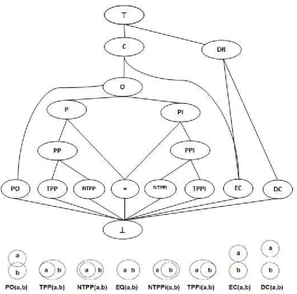
Figure 1: Lattice of the subsumption hierarchy of the basic binary RCC relations (reproduced from

Randell, Cui, Cohn 1994)... 8

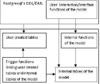
Figure 2: Overview of the system design showing the main elements of the system and their interactions ... 13

Figure 3: Model diagram for main relations ... 14

Figure 4: Exctract from a sketch map added to the database model ... 15

Figure 5: Two different relations realised between an aggregate (X U Y) and a third region (B) but with the same relations between the parts and B - PO(B, X) and PO(B, Y). ... 25

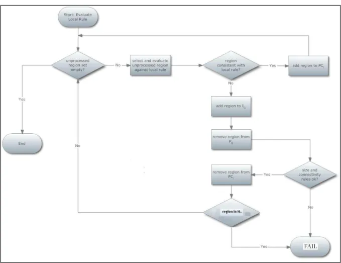
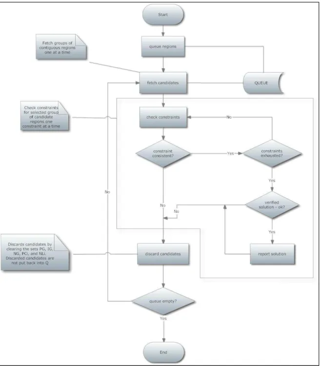
Figure 6: General procedure for evaluating constraint local rules. ... 31

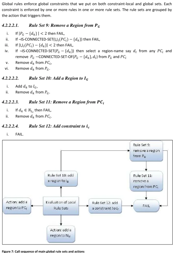
Figure 7: Call sequence of main global rule sets and actions ... 32

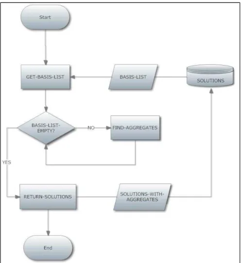
Figure 8: Flowchart of the main process for refining solutions ... 34

Figure 9: Procedure for finding potential parts of a region in the query sketch whose constraints are not satisfiable by the any individual region in the database. ... 35

Figure 10: Three possible choices for the relation between a house and a farm, and between an attachment to the house and the farm. Option (b) is not acceptable since it entails the house overlapping the road (quite unusual). Consequently option (c) is chosen. ... 38

Figure 11: Extracting regions and their relations from sketch maps ... 39

Figure 12: Example sketch map with a group of regions identified in the sketch (red borders). ... 41

Figure 13: Plot of number of regions per solution against number of solutions returned for query 3_1_3 ... 45

Figure 14: Plot of total number of solutions against the number of unique solutions ... 46

Figure 15: Plot of the number of unique solutions returned by the query against number of regions in the query. ... 46

Figure 16: Sketch 2 with two equivalent labelling of regions that lead to ambiguity. Ambiguity of some topological relations is due to symmetry. A and B can both be satisfied by either of the regions Block 1 and Block 2. ... 47

Figure 17: Ambiguity in original sketches carried on to refined solutions ... 48

Figure 18: Original sketch map of sketch 4 (a) and example of a solution with an aggregate region (b). ... 48

1

1.

Introduction

1.1.

Background and Motivation

1.1.1.

Qualitative Spatial Reasoning and Sketch Mapping Applications

On going research efforts in Qualitative Spatial Knowledge Representation (QSKR) and Reasoning (QSR) since the mid 20th century have led to many innovations in Geographic Information Science (GI Science), e.g. spatial query evaluation techniques (e.g. Egenhofer 1997, and Bennett, Isli, and Cohn 1998). Interesting applications such as nuSketch BattleSpace (Forbus 2003) have been built to use combinations of quantitative and qualitative data applying spatial reasoning for some tasks. Such applications provide a basis for research into more general purely qualitative GI applications in areas such as Volunteered Geographic Information and Environmental Modelling.

Many users of geospatial applications may find it easier to work with spatial configurations of entities in the area of interest, using relative metrics as opposed to quantitative details about, for example absolute size, orientation, and location (Egenhofer and Mark, 1995). Tools to support users in this way have been researched as indicated above. These tools are designed primarily for querying spatial datasets in a spatial database with formal expressions of spatial relations specified in a query. The spatial relations in this case have to be computed from the geometric data of the spatial objects stored in the database.

An alternative approach would be to store qualitative representations of spatial datasets in the database, and retrieve the appropriate spatial objects and their relations when required. This would be similar to the approach is presented by Bennett, Isli, and Cohn (1998) where topological relations are pre-computed and stored in the database, and then they are used to evaluate queries. A qualitative model of this kind can allow the storage of spatial data supplied by users in the form of spatial descriptions. Qualitative analyses on this data could include process modelling/simulations (e.g. where people describe a physical process) as in (Forbus 2003), modelling of small spaces (e.g. a small scale farmer’s partitioning of his/her field), way finding, etc.

2

1.1.2.

Motivation and Problem Overview

The above motivations for sketch-based map creation and sharing services not with standing, there are some challenges that have to be resolved even within current models that apply QSR on sketch maps for processing database queries. One major challenge is that most formal theories and models focus only on one aspect of space and their combination is not always easy (Liu, Li, and Renz 2009). Another main problem is that sketch maps are always more abstract than the reality they represent and may contain errors in any of several aspects of the spatial representation (e.g. topology, angle, or shape). Tversky (2002) specifically notes that “it is not trivial to say that people can extract from sketches what sketchers intended”. In some cases, however, systematic errors can be dealt with in systematic ways as proposed by Wang (2009) for angles, curvature and direction, and by Egenhofer and Shariff (1998) for topological relations. Systematic errors in sketch maps may be manifested in several ways including, but not limited to, regularization of angles to right angels, straightening of road curves, exaggeration of size due to the relative significance of depicted features, and hierarchical organization of geographic features (Tversky 2002). Most of these are partly aimed at simplifying the representation in order to minimize the amount of memory and processing required for interpreting the information (Tversky 2003).

A particular form of simplification that may arise during the drawing of a sketch is generalization of information that leads to grouping of features that are conceptually similar or more spatially related. This type of generalization is called aggregation. When a query to a spatial database contains objects (aggregates) that represent aggregated groups of objects, valid solutions to the query may be excluded from the query results because the aggregate object does not match any objects in the database. In such a case, there needs to be a way of recognising and testing when aggregation may cause some results to be rejected, and then to find the objects in the database that correspond to the parts of the aggregate object of the query.

In this thesis, a formal model for topology, namely the RCC-8, is used as the basis for a database model for storing topological information. We use this model to develop a method for refining the solutions of a sketch-based query based on the assumption that some solutions to the query have been excluded as a result of aggregation. The queries in this work are performed against a database containing topological information extracted from other sketches.

1.2.

Research Problem and Objectives

The main objective of this study is to develop a method for refining the solutions of a sketch-based query by searching for groups of objects in the database that together approximately match an object in the query for which no matches were found. The database model will not store any geometric information for the sketches to be analysed. The main objective is achieved by pursuing the following sub-objectives:

i. Develop a database model for topological relations between region objects in a sketch map. The implementation must have query processing algorithms based on the spatial query by sketch (SQBS) paradigm (Egenhofer 1997).

3

1.3.

Outline of the Thesis

5

2.

Literature Review

2.1.

Formalisation of Space

There are many ways to model spatial data qualitatively. The specific elements of any model depend on the desired (or available) level of detail and the properties of the space being modelled, among other things. Surveys in QSKR and QSR have described formal approaches in terms of their theoretical foundations, the spatial aspects being formalised, and the complexity of reasoning over the representations of each approach (Cohn and Renz 2007; Renz and Nebel 2007). For example, logic based approaches such as RCC are distinguished from algebraically motivated ones such as the 9-intersection model, while different models can also be distinguished by the dimension of the entities that are considered as primitive spatial entities of their domains.

Aspects of space can be distinguished in terms of the mathematical theories used to model them. Papadias and Sellis (1993) note that (according to Buisson (1989)):

“… the spaces of interest in spatial reasoning are topological spaces which include only concepts of connectedness and continuity, vector spaces which deal with vectorial dimensions and directions, metric spaces which deal with the concept of distance and Euclidean spaces which admit notions of scalar products, orthogonality, angle and norm.” (Papadias and Sellis 1993, p.2)

6

this affects the direction relations that can be derived between any two regions and sometimes makes it difficult to derive definite direction information using a calculus such as CDC (Egenhofer 1997). While this is the case, direction relations are an important component of qualitative spatial representations used in spatial query evaluation. Section 2.3 below describes how direction relations are used in SQBS and in section 5.4 direction relations are discussed with respect to the number results returned in a query.

Reasoning in QSR is achieved using a variety of approaches of which the most popular are constraint based techniques (Renz and Nebel 2007). These approaches are based on the fact that the relationships between objects can be given in the form of constraints. A constraint over a set of variables consists of a relation and an n-tuple of variables from . The constraint is said to be satisfiable if there exists an instantiation of the variables that is also a member of the relation . Such an instantiation is said to satisfy the constraint . A spatial reasoning problem can then be formalised as a constraint satisfaction problem (CSP) which consists of the set , and a set of constraints over . The desired solution is an instantiation of the variables such that all constraints are satisfied. CSPs are used for verifying the consistency of sets of relations and for comparing different constraint sets as graphs. A formal discussion on formulating and solving constraint satisfaction problems with unary and binary constraints is given in Kumar (1992). A note worthy point is that while binary constraints form edges between variables in the graph of a CSP, unary constraints are viewed as edges from variables to themselves (a loop on the same graph node). However, for simple applications such as the one presented in section 2.3, unary constraints may be excluded from the graph of the CSP because they would first be used to identify possible instances of the variables. This way the process is broken into two parts, the first being elimination of those instantiations of the variables that are not consistent with the unary constraints and then the evaluation of binary constraints.

2.2.

RCC -8

The RCC theory is built on the concept of connectedness defined using one primitive dyadic relation, , that determines for any two regions and whether the regions are connected. The theoretical foundations of the broader theory are rooted in earlier work by Clarke (1981, 1985) – see Randell Cui, and Cohn (1994). In broad terms ( , ), read ‘ connects with ’, is true if and only if the topological closures of and share a common point. In the original publication of the theory, no distinction is made between whether a set is considered as closed, open, or both. The theory provides two additional axioms which make it possible to define a basic set of binary relations. The axioms state that is reflexive and symmetric:

∀ ( , ) …. is connected with itself (reflexivity)

∀ [ ( , ) → ( , ) ] …. If connects with then connects with (symmetry)

The whole set of basic relations derived from can be embedded in a relational lattice with elements ordered in such a way that every higher relation subsumes all lower relations with which it is connected (Figure 1). This means that every relation higher in the lattice implies a disjunction of all lower relations connected to it while a lower relation implies a conjunction of all higher relations connected to it. The following basic relations were defined and presented in the original RCC paper of 1994:

7

∀ ( , ) ↔ ∀ [ ( , ) → ( , )] … ‘ is a part of ’, ∀ ( , ) ↔ [ ( , ) ∧ ¬ ( , )] … ‘ is a proper part of ’, ∀ ( , ) ↔ [ ( , ) ∧ ( , )] … ‘ is identical with ’, ∀ ( , ) ↔ ∃ [ ( , ) ∧ ( , )] … ‘ overlaps ’,

∀ ( , ) ↔ [ ( , ) ∧ ¬ ( , ) ∧ ¬ ( , )] … ‘ partially overlaps ’, ∀ ( , ) ↔ [¬ ( , )] … ‘ is discreet from ’,

∀ ( , ) ↔ [ ( , ) ∧ ¬ ( , )] … ‘ is externally connected with ’,

∀ ( , ) ↔ ( , ) ∧ ∃ [ ( , ) ∧ ( , )] … ‘ is a tangential proper part of ’,

∀ ( , ) ↔ ( , ) ∧ ¬∃ [ ( , ) ∧ ( , )] … ‘ is a non-tangential proper part of ’.

The relations P, PP, TPP, NTPP have inverse relations denoted PI, PPI, TPPI, and NTPPI respectively which means that these relations are non-symmetrical, while the remainder are symmetrical. The inverse of a relation is defined as the converse truth of the relation, so ∀ [ ( , ) ↔ ( , )]. RCC-8 consists of subset of eight of these basic relations that are JEPD. In Figure 1 these are the ones closest to the lower bound of the lattice. Beyond the original interpretation of the primitive relation , Bennett (2000) has given alternative interpretations with respect to different mathematical theories, notably the interpretations in point set topology that distinguish between open and closed sets. In the closed interpretation a region is identified with a regular closed set of points. Two regions are connected if they share at least one point and they overlap if their interiors share at least one point. In the open set interpretation regions are connected if their closures share at least one point, and they overlap if they share at least one point (Bennett, 2000). Both interpretations are consistent with propositions defining the relationships between interiors, boundaries, and closures of spatial regions given by Egenhofer and Franzosa (1991). This relationship between the two formalisms makes it possible to apply either model on the same definition of 2-dimensional spatial regions so that reasoning differs only in the operations employed and not in the formal specification of the input.

8

Figure 1: Lattice of the subsumption hierarchy of the basic binary RCC relations (reproduced from Randell, Cui, Cohn 1994).

2.3.

Spatial Query by Sketch and Spatial Scene Queries

SQBS is a method for performing query operations in spatial databases based on a sketched representation of the desired spatial configuration. According to Egenhofer (1997), traditional query languages are tedious to use and their strict syntax and grammars together with the inherent nature of geographic information (that it is often vague, imprecise, or not standardized) impose a limitation on their usability. He argues that the fact that verbal spatial descriptions are usually ambiguous is a fundamental problem that may lead to misinterpretations.

9

interior and boundary interactions of spatial entities. Cardinal directions are exploited using CDC at two levels. The coarse cardinal directions provide a means for determining the relative direction of one object to another broadly. For example object ! could be north (N) and north-west (NW) of object ". Detailed cardinal directions, on the other hand, say how much north or north-west the object is by calculating the proportion of the objects area (or length for lines) falls into each sector formed by the minimal bounding axes of the referent object.

In contrast with other visual query systems, which require the user to draw close approximations of the desired spatial configurations, SQBS primarily retrieves data based on coarse topological relations and eliminates undesirable results using the four other types of information described above. If no results remain at the end of the query processing, the query may be relaxed by substituting a relation from the query with the union of the relation with its conceptual neighbours (Egenhofer 1997).

A SQBS query is a form of spatial scene query where the query processor attempts to find a spatial configuration that is similar to that expressed in the query. The central question in spatial scene queries is how to establish the associations between the elements of one scene and the elements of another scene (Nedas and Egenhofer, 2008). A spatial scene query comprises a set of spatial objects and relations between the objects. A query is formulated as a spatial CSP. For each spatial object, the properties of the object such as its feature class, shape or size become unary constraints for the query, and the binary relations between the objects become binary constraints of the query.

The evaluation of the query then involves finding configurations in the database that satisfy all the constraints of the query. This is achieved by constructing an association graph which consists of a set pairs of variables (objects in the query) and database objects. The set of pairs are the nodes of the association graph, while the set of combined constraints become the edges of the graph. The construction of the association graph of the CSP involves first resolving the unary constraints by matching query variables to regions. For each variable "_# in the query, add a node $"_#, !_%& to the association graph if object !_% in the database satisfies all the unary constraint of "_#. An edge is added between every pair of nodes $"_#, !_%& and ("_', !₍) of the association graph if the binary constraints between objects !_% and !₍ satisfy the binary constraints between variables "_# and "_' of the query. The final solutions to the query comprise all maximal complete subgraphs (maximal cliques) of the association graphs. Several algorithms for extracting maximal and maximum cliques of a graph have been developed (e.g. Bron and Kerbosch 1973, Tomita et al 2006, Koch 2001).

Solutions obtained from this type query evaluation are not always exact. Three types of solutions are distinguished, namely, complete solutions that are realised from maximum cliques of the association graph when all variables are part of the association graph, incomplete solutions that correspond to maximal cliques with only a subset of the query variables included, and the empty solution when no clique was found in the association graph.

Because there are many possible solutions (many possible association graphs and cliques per graph), to prioritise the results of a query, measures of similarity between the query scene and the database scene have been proposed that take into account three components:

10

ii. A relation similarity component measures the similarity between the binary relations among objects in the query scene and those in the database scene.

iii. A scene completeness component that measures the similarity of two spatial scenes with respect to completeness (i.e. based on number of objects in the query scene, number of objects in the database scene, number of objects matched – or not matched).

The development of the proposed methods for scene similarity assessment was motivated by three psychological insights. First, that people start scene comparisons by locating possible object-matches, that they associate objects so that relations also correspond, and that with a gradual decrease in similarity, very different scenes become irrelevant (Nedas and Egenhofer 2008). A minimum value is imposed on each similarity component which restricts solutions included in the final results that are returned from the query. In this case we want to ensure that all spatial configurations in the database that are potential solutions to the query can be found. If there is an aggregated region in the query sketch then it will reduce the similarity measures of all three components. The present study attempts to reduce this effect by finding database regions that may correspond to an aggregated region in the query sketch.

2.4.

Generalisation and Spatial Aggregation

One problem that has not been tackled by the SQBS and spatial scene query models discussed above is the tendency for people to generalise and schematise perceived environments (Tversky 1993, 2002) and how these generalisations and schematizations are manifested in the sketch maps that people draw. Wang (2009) has made proposals towards alleviating the effects of human schematization and systematic errors in sketch map formalisation. The methods proposed complement the detailed cardinal directions used in SQBS by considering among other things angles and curvature of objects in route maps.

Generalisation is a basic human activity in which unimportant specific aspects of reality are discarded and focus is given to the important ones. The concrete reality can be conversely viewed as a combination of the general and specific aspects that were separated during the generalisation. As a mental process, generalisation involves, among other functions, distinction, combination, and abstraction (Brassel and Weibel 1988) of details from the reality. For sketch maps, the structure captured by the sketches is the structure of the information being conveyed as opposed to the structure of the represented environment. Also, when sketching regions, people impose a hierarchical structure on the features depicted in the sketches emphasizing those with a larger environmental scale (Tversky 2002). From this it may be construed that the process of spatial generalisation as human activity is also impacted by the hierarchical organisation of information internalised by an individual or by at least by the process that generates this hierarchical representation.

11

there is need for a non-numerical model for deciding how regions should be aggregated as spatial entities based on non-homogeneous but possibly related criteria.

From a topological perspective, the aggregation of spatial regions in a spatial scene presents some problems with respect to the consistency of the configuration obtained. This problem has been investigated by Tryfona and Egenhofer (1997) but no complete solution for the purely qualitative case has been found in the literature. Based on the 4-intersection model, a variation of the earlier cited 9-intersection model, this result is derived from an analysis of the interaction of the interiors and boundaries of the aggregate region and a third region on the one hand, and between the parts and the third region on the other.

13

3.

Test Model Design

The model was implemented in the Postgresql Database Management System. All functionality is written in the built-in procedural language PL/PGSQL which presented a few challenges as it is limited in terms of data structures as well as being a purely procedural language without support for session (global) variables. However, the implementation was sufficient for testing the query system with a variety of input queries on different topological configurations extracted from sketch maps. Objects in the sketches, which are interpreted as 2-dimensional regions in the plane, are represented by identifier labels or ‘region names’. Region names are stored as text fields of variable size no more than 48 characters in length. All operations on data in the model are thus performed using references to the region names.

3.1.

Database Design

Internally, each region name is associated with a unique region id (reg_id). User tables can be created and then associated with the internal structure by declaring one of their columns as a column of region names. This is achieved by invoking the function, set_rcc_table(table_name, column_name), which alters the column to a 48-character variable length text field with unique values and sets a trigger to execute before each one of the three row-level operations insert, update, and delete. set_rcc_table also changes the name of the column to the_rcc_region. Once the link has been established, a user can manipulate his/her user tables using Postgresql’s standard SQL statements and other functions. All changes to values in the column of region names will be reflected in the internal tables of the model. Other functionality of the model is accessible through several user interface functions discussed in the following sections. Figure 2 shows an overview of the overall system design for the implementation.

Figure 2: Overview of the system design showing the main elements of the system and their interactions

14

later changes made to the internal program code did not require changing the user interaction methods or the functions that implement them.

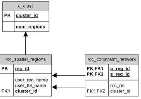
The table c_clust keeps track of all regions that are altogether contiguous. Each record of c_clust consists of a cluster identifier number and the number of region names in the cluster. Upon insertion into the database, a region is assigned to the default cluster (cluster_id is 1). The default cluster is associated with all isolated regions. A region is subsequently removed from a cluster and added to another cluster when a constraint has been imposed on it with other regions in the database such that the region is no longer connected to any member of the original cluster. Two clusters are combined into one if any two regions, one from each cluster, become connected.

Finally, the table rcc_constraint_network stores records of basic RCC-8 constraints over the set of regions corresponding to the region names. Each constraint is stored as an ordered pair of region identifiers and a RCC 8 relation name.

Figure 3: Model diagram for main relations

There are several other tables that support data processing functionality. The most important of these are rcc_rel_comp, rcc_rel_compb8, rcc_u_constraints, rcc_b_constraints, rcc_qryreg_assoc, qry_soln_graphs, and qry_usr_soln.

rcc_rel_comp, rcc_rel_compb8 are the RCC-8 composition table for the eight basic relations and the composition table for all possible unions of RCC-8 relations respectively. The latter is computed from the former using the algorithm implemented by Fehling, Nebel, and Renz (1998). rcc_u_constraints and rcc_b_constraints are used to store unary and binary constraints, respectively, for each query. rcc_qryreg_assoc and qry_soln_graphs are used for storage of intermediate results during query processing, while qry_usr_soln is used as a template for presenting the final results.

3.2.

Data Input Methods

15

subsequently inserted regions should not be added to the currently selected sketch map. An insertion without a prior selection of a sketch map using use_sketch(sketch_name) will fail. Three functions that take as arguments a binary constraint over two region names in the database enable the input and manipulation of constraints imposed on regions in a sketch. The function related_regions(primary_region, secondary_region, relation) adds the following constraint to the database: primary_region { relation} secondary_region. For example, if region X is a tangential proper part of region Y, then related_regions(X, Y, TPP) inserts X {TPP} Y into the table rcc_constraint_network.

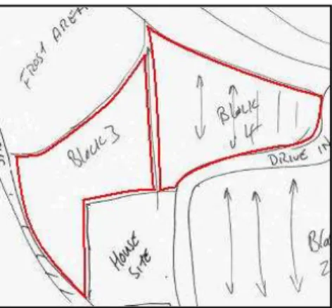
Figure 4: Exctract from a sketch map added to the database model

The function unrelated_regions(primary_region, secondary_region) removes the constraint imposed by related_regions on the given pair of regions. Since the database does not explicitly store constraints for which the corresponding relation is DC, calls to the function related_regions with the relation DC simply trigger a call to unrelated_regions. Specifically, these two functions are responsible for maintaining the cluster index by updating it whenever regions move between clusters.

SELECT use_sketch('KiwiFarm 1');

INSERT INTO farms(name, description, the_rcc_region) VALUES ('Block 3', 'Farm division block 3', 'S1Block3'); INSERT INTO farm_properties(feature, name, value)

VALUES ('S1Block3', 'Category', 'spatial organisation'); INSERT INTO farm_properties(feature, name, value)

VALUES ('S1Block3', 'Feature', 'blocks');

INSERT INTO farms(name, description, the_rcc_region) VALUES ('Block 4', 'Farm division block 4', 'S1Block4'); INSERT INTO farm_properties(feature, name, value)

VALUES ('S1Block4', 'Category', 'spatial organisation'); INSERT INTO farm_properties(feature, name, value)

VALUES ('S1Block4', 'Feature', 'blocks');

SELECT end_sketch();

SELECT related_regions(get_region_id('S1Block3', 'farms'), get_region_id('S1Block4', 'farms'), 'EC');

16

Listing 1 above shows the SQL script that adds data about the highlighted regions in Figure 4 to the database. The first line instructs the database to associate all data about regions inserted from that point with the sketch named ‘Kiwi Farm 1’. The reference to the sketch does not have to exist prior to the call, but if the name was already added to the database, then the existing reference is used. The last but one call indicates to the system that the input has finished. Any data added after this will not be associated the current sketch and if no other sketch is specified, input will fail for any value of the column the_rcc_region. The final line instructs the system to add a constraint (EC) between the two recently added regions. The table farm_properties here illustrates that other tables can be linked to a table with region names and data in those tables may be used during a query as seen in the coming sections.

The last function update_region_constraint(primary_region, secondary_region, relation) allows constraints to be edited in a consistent way by ensuring that no constraint is previously imposed on the given pair of regions prior to an update. Basically, an update is a sequence of two function calls, first to unrelated_regions and then related_regions.

3.3.

Consistency and Path-consistency

Consistency checking is used to maintain the database in a consistent state every time a constraint is added or removed. Because path-consistency implies consistency in a basic RCC constraint network, we only apply a path-consistency algorithm when testing for consistency. Path-consistency also plays the role of ensuring that a set of constraints is complete by adding to the set the inverses of all constraints in the set and for every constrained object the constraint that the object equals itself. In the implementation of the model, path-consistency is checked using a variation of Van Beek’s path-consistency algorithm for CSPs (van Beek 1992). The algorithm used was proposed by (Stocker and Sirin 2009) and uses the recursive procedure ) $ _#%, & to verify the path-consistency at the node (*, +) of the CSP but allows for the empty and the universal relations to be ignored.

17 Function: PATHCONSISTENCY(Θ)

Input: Set Θ of binary RCC-8 constraints over a set of variables V. Local: Set G of binary RCC-8 constraints over V.

Output: Path-consistent set equivalent to Θ, or NULL if inconsistency is detected. 1. if Θ = Ø then

2. return Θ

3. end if

4. G ← complete(Θ) 5. if G ≠ Ø then

6. Q ← {Rij | i, j ϵ V and Ø≠ Rijϵ G}

7. while Q ≠_Ø do

8. G ← ISCONSISTENT(G, Q, POP(Q))

9. if G = Ø then

10. Q ← Ø

11. end if

12. end while

13. end if 14. return G

Function: ISCONSISTENCT(G, Q, Rab)

Input: Set G of binary RCC-8 constraints over a set of variables V, FIFO set Q of binary RCC-8 constraints over V,

Binary constraint Rab on variables a, b ϵ V.

Output: Set equivalent to G that is path-consistent at Rab, or NULL if inconsistency is detected.

1. for each Rbc ϵ G, c ≠ Ø, a, b do 2. G ← RELADD(G, Q, Rab o Rbc)

3. if G = Ø then

4. return G

5. end if

18 Function: RELADD (G, Q, Tac)

Input: A set G of binary RCC-8 constraints over a set of variables V, FIFO set Q of binary RCC-8 constraints over V,

Binary constraint Tac on variables a, c ϵ V derived from the composition over (a, b) and (b, c).

Local: Uac ,Vac orginal and refined constraint on pair (a, c).

Output: Path-consistent set equivalent to G, or NULL if inconsistency is detected. 1. if T = Ø then

2. Return G

3. end if

4. Uac← {Rij | i = a, j = c, Rijϵ G}

5. if Uac = Ø then

6. Vac ← Tac

7. Else

8. Vac ← Tac∩ Uac 9. if Vac = Ø then

10. G ←Ø

11. return G

12. end if

13. if Uac = Vac then

14. return G

15. end if

16. G ← G - {Uac} 17. end if

18. G ← G U {Vac} 19. Q ← Q U {Vac}

20. RELADD (G, Q, inverse(Vac))

21. return G

Algorithm 1: PATH-CONSISTENCY algorithm (from Stocker and Sirin, 2009)

3.4.

Database Query

Queries on the data are formulated in two ways. A simple query may be an SQL select query to retrieve the set of region pairs that are constrained by a certain relation or to view the relation that is constraining a pair of regions. In addition, a simple query may be combined with other SQL queries to produce more complex but perhaps more useful results.

The second type of query is based on the query by sketch paradigm. As in Nedas and Egenhofer (2008), a sketch-based query is composed of two parts: A set of unary constraints on each variable from a set of variables , and a set of binary constraints on members of the Cartesian product V×V. Such a query may have several solutions and a solution to the query may be complete, incomplete, or empty.

3.4.1.

Relational Queries

19

3.4.2.

Sketch-based Queries

The sketch-based query is modelled after Nedas and Egenhofer’s spatial query with a few differences. According to their paper a spatial-scene query “has two major components: objects and relations among the objects” (Nedas and Egenhofer 2008). The analysis and evaluation of the query involves matching properties of objects expressed in the query and their binary constraints with those of objects in the database. These correspond to unary and binary constraints for the query respectively.

Each sketch that will be used to query the database must first be formally analysed to extract the topological relations among the objects depicted in the sketch. A manual process for achieving this is used in this study.

3.4.2.1.

Sketch-based Query Presentation

Queries to the database are constructed by a series of calls to two functions, one for setting unary constraints and another for setting binary constraints for the query. Unary constraints are given as any SQL statement returning sets of region names.

The function unary_qry_constraint() must be called once for each object (variable) in the query sketch. Any variable not passed explicitly to the query system will not be processed. The function unary_qry_constraint() takes three arguments, namely, a variable name, the table from which regions must be fetched, an SQL statement as indicated above. As each variable is added, it is assigned a position in natural order starting from 1 for the first variable. Apart from the requirement that the SQL query must return a set of region names, the manner in which it is constructed and/or processed by the database backend is not influenced by the design of the query processing procedures. Consequently, there is no straight forward way to isolate the individual components or attributes of the unary constraints.

The function binary_qry_constraint(string_of_binary_constraints) must be called exactly once before executing the query. This sets the binary constraints placed upon the query variables. Binary constraints are given as a string of the following format:

primary_region secondary_region relation [AND primary_region secondary_region relation […] …]

3.4.2.2.

Sketch-based Query Processing

Once the query variables and constraints have been set, the query is executed by calling the function rcc_eval_qry(). This function takes a Boolean argument specifying whether constraint relaxation for binary constraints should be attempted. The main processes that occur include query validation, variable to region name matching, creation of the association graph from each set of matches, generation and storage of viable solutions from the association graph.

3.4.2.2.1.

Query Validation

20

The function returns a matrix representing a set of path-consistent constraints, or NULL if the constraints specified are inconsistent. But as a result of the way the path-consistency function processes the CSP, if the constraint between a pair of regions could not be discovered, this particular constraint is simply made NULL as opposed to removing the concerned regions from further analysis or failing the validation. This may contrast however with the Egenhofer approach because in that case constraints are not atomic but elements of Cartesian products several constraint sets.

3.4.2.2.2.

Variable Region Matching

For each variable execute the associated SQL statement to retrieve the region names that belong to tuples returned from executing the SQL statement. This results in the creation of a list of matches between variables and region names. This match-list is then used to create a set of possible solutions to the query. Each potential solution set is a subset of the Cartesian product × in which each variable appears at most once, and each region appears at most once. This removes unnecessary steps when checking binary constraints. The condition set by Nedas and Egenhofer, however, only stipulates that each variable must appear at most once in any given association graph since in their approach only a single association graph is created for all possible matches.

As shown in Algorithm 1 the procedure for constructing solution match sets is iterative. Starting with one variable, each variable-region match is placed in its own solution match set. Then for each set, new sets are created by including every match of the subsequently selected variable into a new solution set. This process is repeated while ensuring that a match is not added to a solution set if another match with the same region was previously added. Additionally, the algorithm used restricts the regions that can be added to be from the same sketch. This introduces a bias in the content of results that can be obtained since only sketches for regions that matched the first variable will be included in any solution set. For purposes of our experiment this wasn’t a problem because the number of sketch maps was small and the types of features used was limited so that every sketch map had at least one feature of the popular feature types.

Algorithm: MAKE-SOLUTION-SETS

Input: Set L of variable-region pairs (v, u) s.t. v ϵ V and u ϵ D the set of region names in the database.

Local: newLSS lists of members of L. Output: Set S of lists of members of L. 1. S ← {Ø}

2. for each v ϵ V do

3. for each LSS ϵ S do

4. for each (v, u) ϵ L do

5. if (u is not already in LSS and LSS does NOT contain a

region from DIFFERENT sketch as u)

6. newLSS ← LSS U {(v, u)}

7. S ← S U {newLSS}

8. end if

9. end for

10. if newLSS ≠ Ø then

11. S ← S - {LSS}

12. end if

13. end for

14. end for

21

The order in which variables are processed in the procedure determines the number and content of the output solution match sets and therefore of the final solution. This is because of the restrictions on inclusion stated above, and the possible variations in the number of regions matched to each variable and vice-versa. The algorithm mitigates this effect slightly by processing variables with the highest number of matches first. This ensures that for each variable, there is a higher possibility to find at least one solution set to which it can be included. A bad case is when all variables match exactly one region and some regions are repeated, in which case only the first encountered variable matching the repeated region is included in the solution.

3.4.2.2.3.

Construction of the Association Graph

The association graph is constructed in a similar manner as Nedas and Egenhofer’s although our approach is based on building smaller sets of potential solutions. Whenever a constraint is NULL, it is excluded from the final solution. So, for any pair of variable-region matches, if the corresponding constraints are NULL, then they cannot be in the same solution. The resulting association graph is represented as a matrix of the same dimension as the query constraint graph. Whenever the constraint between regions in the database did not satisfy constraint between variables matched to those regions, the association graph entry corresponding to the joint constraint between the matches is set to NULL.

3.4.2.2.4.

Generating Solutions

The final query solutions are created from the solution sets using a clique enumeration procedure. The maximal clique algorithm version 2 of Bron and Kerbosch (1973) is applied on each association graph extracting cliques that are either maximal or maximum (Algorithm 3). Each clique is a solution to the original database query. The solutions are stored in the table qry_soln_graphs, each with a reference to the solution set that generated it and a unique integer to identify the solution.

The solutions of the query are however not unique because of several obvious reasons. Firstly, the construction of solution sets allows for redundancies since two solution sets may have exactly the same variable-region matchings for a proper subset of the total number of variables. This is certainly the case where there are no unary constraints on any of the variables and each variable is matched with every other region in the database. Secondly, because we enumerate all maximal cliques of every solution graph, even those solution sets that do not have exactly the same set of regions, may end up giving the same solution. The alternative approach to find only the maximum clique is not anymore effective since it may instead reject valid (incomplete) solutions with regions that more closely match the regions given in the query in favour of a poorly matching complete solution.

3.4.2.2.5.

Presentation of Results

22 Algorithm: MAXIMAL-CLIQUES

Input: Graph G=(V, E).

Local: FIFO set Q of binary RCC-8 constraints over V.

Output: Path-consistent set equivalent to Θ, or NULL if inconsistency is detected. Function: extract_maximal_cliques(C, P, X)

Input: clique to be extended C, set P of candidates vertices that are all connected to vertices in C, set X of vertices already processed and now excluded from the current extension.

Local: Pivot point up used by the branch and bound method to truncate the search tree.

Output: Set S of maximal complete subgraphs of G. 1. if P = Ø then

2. Report C as maximal clique 3. end if

4. for each v ϵP U X do

5. if |NEIGHBOURS(v)| < MIN({|NEIGHBOURS(w)|; w ϵ P U X }) then

6. up← v

7. end if

8. end for

9. for each u ϵP do

10. if NOT u ϵ NEIGHBOURS(up) then

11. P ← P-{u}

12. Cnew ← C U {u}

13. Pnew ← P ∩ NEIGHBOURS (u) 14. Xnew ← X ∩ NEIGHBOURS (u)

15. extract_maximal_cliques(Cnew,Pnew,Xnew)

16. X ← X U {u}

17. end if 18. end for

19. Return

Algorithm 3: Bron-Kerbosch maximal clique algorithm version 2 (from a note on clique enumeration algorithms, Cazals and Karande 2008)

Because redundant solutions always come up, there is another function rcc_return_unique(), which returns only unique solutions by grouping all equivalent solutions together and presenting them only once. Both functions return solutions in the same format including a solution number, and sketch id. After all solutions have been returned, a subsequent call to either of the functions loops back to the first solution and so on.

3.4.2.3.

Illustration of Sketch-based Querying with an Example

23

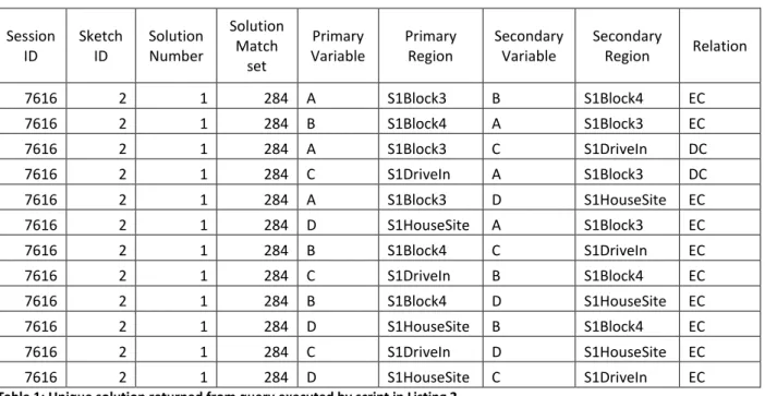
model not to apply constraint relaxation during execution. The statement SELECT * FROM rcc_return_unique(2) fetches next available unique solution of size greater than or equal to two

from the query results. The output for the query is shown in Table 1.

Session ID Sketch ID Solution Number Solution Match set Primary Variable Primary Region Secondary Variable Secondary

Region Relation

7616 2 1 284 A S1Block3 B S1Block4 EC

7616 2 1 284 B S1Block4 A S1Block3 EC

7616 2 1 284 A S1Block3 C S1DriveIn DC

7616 2 1 284 C S1DriveIn A S1Block3 DC

7616 2 1 284 A S1Block3 D S1HouseSite EC

7616 2 1 284 D S1HouseSite A S1Block3 EC

7616 2 1 284 B S1Block4 C S1DriveIn EC

7616 2 1 284 C S1DriveIn B S1Block4 EC

7616 2 1 284 B S1Block4 D S1HouseSite EC

7616 2 1 284 D S1HouseSite B S1Block4 EC

7616 2 1 284 C S1DriveIn D S1HouseSite EC

7616 2 1 284 D S1HouseSite C S1DriveIn EC

Table 1: Unique solution returned from query executed by script in Listing 2

Listing 2: Script for a sketch-based query corresponding to Figure 4

SELECT rcc_clear_qry();

SELECT unary_qry_constraint('A', 'farms ', 'select distinct a.the_rcc_region as the_rcc_region from farms a, farm_properties b

where a.the_rcc_region = b.feature and (b.name = ''Feature'' and b.value = ''blocks'')

');

SELECT unary_qry_constraint('B', 'farms ', 'select distinct a.the_rcc_region as the_rcc_region from farms a, farm_properties b

where a.the_rcc_region = b.feature and (b.name = ''Feature'' and b.value = ''blocks'')

');

SELECT unary_qry_constraint('C', 'farms ', 'select distinct a.the_rcc_region as the_rcc_region from farms a, farm_properties b

where a.the_rcc_region = b.feature and (b.name = ''Feature'' and b.value = ''driveways'')

');

SELECT unary_qry_constraint('D', 'farms ', 'select distinct a.the_rcc_region as the_rcc_region from farms a, farm_properties b

where a.the_rcc_region = b.feature and ((b.name = ''Feature'' and b.value = ''houses'') and (a.description ~* ''farm house''))

');

SELECT binary_qry_constraints('A B EC AND A C DC AND A D EC AND B C EC AND B D EC AND C D EC');

SELECT rcc_eval_qry(false);

24

3.5.

Summary

The design of the model presented here is simple in comparison with the original SQBS model of Egenhofer on which it is based. It does not take into account direction information and assumes that topological relations are simple and known exactly. This simplicity results in a larger set of results being returned for any given query. The inclusion of direction relations and detailed topological relations would narrow down the results because the constraints would be stricter.

25

4.

Refining Solutions

As observed in some sketch maps obtained from an experiment done in this study and with the insights from psychology and GI Science, it is evident that spatial aggregation is a process that may be performed by people drawing sketch maps. The aggregation may be intentional, motivated by the application of the map, or it may be a consequence of an attempt to abstract from the reality only those aspects that are of interest, thereby simplifying the representation. Although it was not possible, in this study, to establish the extent to which aggregation may be used in the map sketching process, its occurrence presents challenges during query processing with sketch maps, since it is not possible to know, beforehand, whether constraints on a sketched region in a query can be satisfied by the combined constraints of a group of regions in the database.

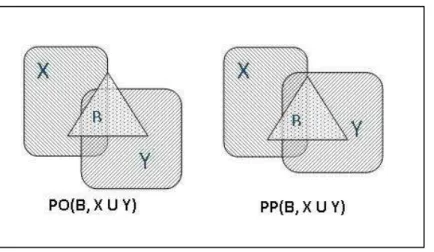
In this chapter, an extension to the test model described in chapter 3 is presented. The purpose of the model is to identify possible situations where a query variable may represent an aggregation of several regions in the database and then discovering a set of spatial regions in the database that satisfy the topological constraints of the aggregate with other regions in the query result. The regions so found become the parts of the aggregate and can be included in the solution in its place. As observed by Tryfona and Egenhofer (1997), the task of determining the consistency between the relations of an aggregate region and a third region, and the relations between its part and the third region is not trivial, especially for regions with disconnected parts. In fact, for some configurations it is impossible to determine consistency based only on course topological relations. As such, the solution proposed does not provide a definitive answer to the question, whether a group of regions in the database maybe aggregated to satisfy a query, but rather an approximate answer. The result is approximate in the sense that, while all regions identified may not introduce inconsistency in the overall configuration, there are relations for which we cannot determine, based on topology alone, whether the given combination of regions contains regions that facilitate the satisfaction of a particular query constraint. For example, if the aggregate contains another region, then if all parts of the aggregate partially overlap this region it is not possible to know whether the parts together cover this region completely or only partially (Figure 5).

Figure 5: Two different relations realised between an aggregate (X U Y) and a third region (B) but with the same relations between the parts and B - PO(B, X) and PO(B, Y).

26

Because of these assumptions, we only attempt to find such aggregates if the number of matches in the solution’s match set equals the size of the query or the size of the query minus 1. The first two assumptions are imposed to reduce the number of conditions that must be tested to determine whether the binary constraints of an aggregate’s parts are consistent with the binary constraints of the aggregate (section 4.2.2 below). Additionally, if we assume that there is more than one aggregate region then there must be appropriate heuristics for discovering them, deciding how to combine database regions, and testing the consistency of the binary constraints between the groups of database regions with constraints of the aggregated query regions. These problems are beyond the scope of this study.

4.1.

Analysis of the Problem

To determine whether a variable in the sketch query may be referring to a group of contiguous regions, we analyse the solutions generated during the initial query processing. The building of solution sets provides a pattern in which the results can be studied further. Consider a query with / variables. For each set of solutions with 0 common variable-region matches, the 0 common variable-region match subset will be called a basis for that set of solutions. Every basis in the set of solutions is itself an incomplete solution. The question is, given a set of incomplete solutions, whether we can generate a complete solution from the basis and a certain combination of variable-region matches or by introducing new variables to the query that correspond to parts of an aggregate region.

If there are / − 0 variable-region matches that, if included in the basis, would lead to a complete solution, then we should already have the complete solution. So, in this case, there aren’t any such matches and of the / − 0 matches in each of the incomplete solutions there are some that fail to satisfy one or more binary constraints of the query.

For the case 0 = / − 1, we want a query variable ) that satisfies the following conditions:

i. For each solution match set under consideration, ) is matched with a different region or it is not matched at all;

ii. For each solution, the exclusion of ) leads to the largest possible solution for the corresponding solution match set (a solution of size / − 1 for this case or 0 in general); iii. For each solution, the inclusion of ) in the solution leads to the exclusion of at least one

other variable in the corresponding solution match set.

Condition (i) is a consequence of the choice of a basis. Since all solution match sets have the same basis of size / − 1, the only different match is the one for variable ). The second condition (ii) ensures that we do not have a complete solution using this basis and makes a point that any matching of ) does not lead to a complete solution. Similar to condition (ii), condition (iii) provides a stronger test of the constraints of the variable ) with respect to the basis – that is, every match for ) is inconsistent with the constraints of at least one region in a consistent solution.

27

In the RCC theory, the 9!0 function can be used to define the aggregate of two regions and . The function is defined as (Bennett 2000, Randell, Cui, and Cohn 1992):

∀ 9!0( , ) = ↔ ∀:[ ( , :) ↔ ( , :) ∨ ( , :)]

To which is added the constraint that the parts making the aggregate must be contiguous proper parts of it:

∀ [9!0( , ) = → ( , ) ∧ ( , ) ∧ ( , ) ] (i)

And finally the aggregate with more than two parts is constructed by summing a two part aggregate with another aggregate or other region making sure that condition (i) above holds. The constraint above is consistent with the definitions of the basic RCC relations and the 9!0 function as given in the original paper on RCC since ( , ) → ∀:[ ( , :) → ( , :) ].

4.2.

Model Components for Processing Database Region Names

The first condition set on the regions to consider is that they come from the same sketch map as the regions in the original solutions. The second condition is that they must be contiguous. This is necessary because dealing with disconnected regions in spatial aggregation is more complex and beyond the scope of this thesis. The cluster structure of the current model is used as a first elimination strategy by retrieving only regions in the same cluster. Regions that are already in the basis are excluded, while regions which were previously matched to ) and were included in at least one solution are given priority since they satisfy at least one constraint of ).

4.2.1.

Region Name Sets

The model makes use of two groups of sets of region names, namely, constraint-local sets and global sets. There are two constraint-local sets for each binary constraint * of the variable ): _#, which is a set of regions that together or individually satisfy the constraint *, and _<=, the set of regions necessary for constraint * to be satisfiable by the regions in _# so that _<=is a subset of _#. Since the set _> is processed all at once, regions are never removed from _<= but can be removed from _# if they have been identified as regions that cause inconsistency elsewhere.

Global sets facilitate the decision of success or failure for the process. The set PG contains all regions selected for inclusion in the solution which must be a contiguous (connected) set; the set _> contains members of every _<= in the model; and the set I_G is the set of inadmissible regions – which have been determined to be inconsistent with some constraint of ). The sets PG and IGare disjoint while _> is a subset of PG. Additionally, there is a variable *_Bthat is only instantiated when a constraint is found to be inconsistent, so that if *_B is not empty, then the process has failed. Formally, for C constraints we have the following restrictions on the sets:

# ⊆ >, 1 ≤ * ≤ C (i) <= ⊆ #, 1 ≤ * ≤ C (ii)

>⊆ > (iii)

>= F(#G <= (iv)

28

As indicated above, regions are selected from the same cluster and added to the set PG. For each constraint of ), each region in P_G is then processed against a set of rules and the information in the constraint-local and global sets. The result is that a region is either consistent or inconsistent with the constraint. An inconsistent region will be added to _> and a consistent region to _#. The process fails when either a region in _> is chosen to be added to _> or when _# fails to satisfy the corresponding constraint *.

4.2.2.

Rule Sets

The processing of the regions in the sets is done by evaluating a set of rules on a constraint level and on a global level. Constraint-local rules apply to each constraint differently depending on the relation implied by the constraint and determine the consistency of _# with respect to corresponding constraint *. The approximate nature of the result is inherent in the local rule sets because it is here that local consistency is determined. Global rules are applied the same for every constraint and are used to determine the consistency of the whole configuration.

Rules are grouped into rule sets which must all be executed whenever the rule set is invoked. Rule sets are a combination of rules and actions, and some contain only actions but they are all treated the same way during execution. The actions are operations on some given data structure of the model, like the constraint-local sets described in the previous section, with a specific data input such as a query constraint and database constraint. In contrast, rules are conditional statements that cause a specific action or group of actions to be invoked based on the evaluation of the condition.

4.2.2.1.

Constraint-local Rules

There are eight constraint-local rule sets which correspond to the eight basic relations of the RCC-8 model. These rules are used to evaluate whether a region in _> is necessary for constraint *, or it is consistent, inconsistent, or irrelevant to the constraint. In the following, B is a variable in the query with constraint _KL with variable ) which we want to verify for a group of database regions and 4_' ∈ _> is any region in the database that is a potential part of ).

4.2.2.1.1.

Rule Set 1:

NO = P

i. If _STL= then add 4_' to _#, ii. If _STL∈ then add 4_' to _>,

iii. If | _#| < 2 then label constraint _KL as inconsistent and instantiate *_B to _KL.

4.2.2.1.2.

Rule Set 2:

WO = P

i. If _STL∈ then add 4_' to _#, ii. If _STL∈ then add 4_' to _>,

iii. If ∀4₍ ∈ _>, _SXL≠ then label constraint _KL as inconsistent and instantiate *_B to _KL, iv. If ∀4₍ ∈ _#− {4_'}, _STL= ∧ _SXL = then add 4_' to _<= and update _>.

4.2.2.1.3.

Rule Set 3:

\] = P