Tracking Error of Exchange-Traded Funds:
Evidence from the UK
Maastricht University
NOVA SBE
René Dingelstad (i6020178, 797)
MSc Financial Economics & Master in Finance
Supervisors:
Melissa Prado
List of Contents
List of Figures 3
List of Tables 4
Abstract 5
Introduction 6
Literature Review 10
Fundamentals of Exchange-Traded Funds 10
Exchange-Traded Funds and Index Funds 14
Exchange-Traded Funds Price Discounts and Premiums 18
Tracking Error in Exchange-Traded Funds 20
Literature Review Conclusion 25
Sample and Research Design 26
Methodology 31
General Performance 31
ETF discount and premium 32
Tracking Error 32
Correlations 35
Determinants of the Tracking Error 36
Results 38
General performance 39
NAV discrepancies 44
Tracking Error 51
Method 1 - Simple Tracking error 51
Method 2 - Mean Absolute Tracking Error 53
Method 3 - Standard Deviation of Return Differences 56
Method 4 - R-Squared 57
Method 5 - Standard Error 59
Market Volatility 60
Determinants of the tracking error 63
Discussion and Implications 66
Conclusion 69
Appendix 72
Appendix A - Full Sample 72
Appendix B - Code 74
References 75
List of Figures
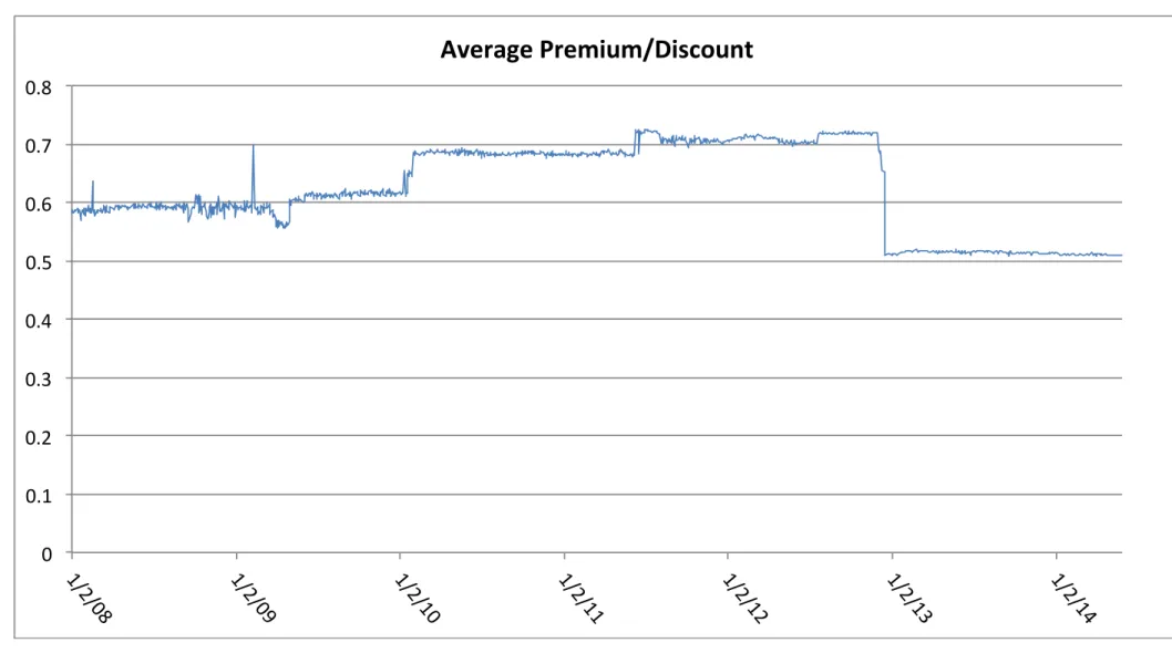
Figure 1: Equity Average Premium/Discount 45
Figure 2: Commodity Average Premium/Discount 46
Figure 3: Bond Average Premium/Discount 47
Figure 4: Total Average Premium/Discount 48
Figure 5: Average Tracking Error 52
Figure 6: Histogram for Average Tracking Error 52
List of Tables
Table 1: Sample Characteristics 28
Table 2: General Performance Comparison 40
Table 3: Return Correlations of ETF on Benchmark Index 43
Table 4: Beta Coefficient of Regression 43
Table 5: Simple Tracking Error 53
Table 6: Absolute Tracking Error 54
Table 7: Standard Deviation of Return Differences 57
Table 8: Coefficient of Determination (R2) 58 Table 9: Standard Error of Regression 59
Table 10: Market Volatility Correlations 61
Table 11: Tracking Error Regression 64
Table 12: Adjusted Tracking Error Regression 65
Abstract
Introduction
Exchange-traded funds (ETF) are arguably the best way for investors to expose themselves to one specific market or sector. The need for international and industry diversification is common knowledge among investors and a reason for the high use of ETFs. Sophisticated investors have understood the need to diversify in order to avoid idiosyncratic risk and have generally done so for many years. By having a well-diversified portfolio with positions in multiple asset classes and with a broad geographic focus, idiosyncratic risk can be diversified away, leaving just the exposure to market risk. Diversification was previously achieved by buying the different assets individually or by investing in mutual funds. Since the introduction of exchange-traded funds however, diversification has gotten easier and more accessible for investors (Gastineau, 2001). As soon as investors understood the advantages of ETFs, the use of ETFs boomed. During the past decade, partially at the expense of index mutual funds, exchange traded funds saw a massive inflow of funds and an explosive growth in trading volume and turnover (Agapova, 2011). The first ETF listed on the LSE was introduced in April 2000, a fund tracking the FTSE 100 index, and by 2004 there were 14 ETFs listed on the exchange. In April 2014, 10 years later, 1043 exchange-traded products were listed on the London Stock Exchange (London Stock Exchange, 2014). Daily turnover went from about £10 million per day in 2004 to more than £650 million per day in 2014. The total turnover in the ETF market on the LSE was over £12 billion in April 2014 alone. The London stock exchange is particularly important because it is the largest ETF exchange in Europe by volume (London Stock Exchange, 2013). As of November 2013 the exchange accounted for more than 30% of European on-exchange trading in ETFs.
between the market price and the underlying value of the fund (Gastineau, 2001). They can do so either by creating, or by redeeming an ETF depending on whether it is trading at a premium or at a discount respectively. Next to efficient pricing, ETFs are also priced continuously and can be traded at any time during trading hours, making them more attractive than traditional (index) mutual funds on that respect (Gastineau, 2001). Next to efficient pricing and straightforward trading, investing in ETFs comes with low transaction costs and extremely low management fees due the funds’ completely passive nature (Mussavain and Hirsch, 2002). Contrary to index futures, ETFs are not a derivatives contract, do not have a maturity date and do not require margin management. These advantages of ETFs over other investment products are only relevant however if the ETFs actually manage to track their index well and deliver virtually identical performance as their benchmark. If an exchange-traded fund fails to replicate its benchmark the ETF does not serve its point and irrespective of its advantages the product will not be used. This tracking ability of exchange-traded funds is thus a critical issue and one that will be evaluated in detail in this study. Funds’ ability to replicate the index can be approximated using the concept of a tracking error. If the tracking error of an ETF is high it indicates that the fund does not actually deliver the return and exposure the investor is looking for. When this tracking error is significantly big and consistent over time, investors may decide not to use ETFs as their preferred security to obtain index exposure but rather choose futures or index mutual funds. Hence it is fair to say that the tracking error is a crucial factor for the existence of exchange-traded funds.
The academic literature on exchange-traded funds is growing as the importance and use of ETFs keeps increasing. Nevertheless, there is still plenty of room for more research on exchange-traded funds. The massive increase in trading volume and turnover of ETFs is already a justification for more research on its own, but the UK market calls for more research itself too. Despite the 30% market share of the LSE in ETF trading, making it the largest in Europe, there has not been any academic research on the performance of these UK-listed exchange-traded funds yet. In particular more research on their tracking performance and the sources of a possible tracking error is desired. Previous studies such as Shin and Soydemir (2010) and Buetow and Henderson (2012) found that ETFs generally track their benchmark quite well and that discrepancies are only of a very small magnitude. Other papers such as Milonas and Rompotis (2006) and Chu (2011) found the exact opposite and concluded that many ETFs had serious issues in tracking their benchmark index. Similarly to disagreements about the size of the tracking error itself, previous research has not always agreed on tracking error determinants either. Depending on the models they used, researchers found different sources for the tracking error. Milonas and Rompotis, Rompotis (2009) and Chu find that the expenses have a significant impact on tracking error, but do not always agree on the direction of the effect. Rompotis (2012) and Shin and Soydemir on the other hand do not find any significant relationship between the expense ratio and the tracking error. The latter two papers find other factors that have a significant impact on the tracking error however, such as the bid-ask spread, risk, absolute price premium and daily price volatility.
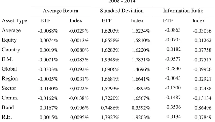
It is found that ETFs listed on the LSE generally perform quite well on most fronts. They offer a return very close to the benchmark return but at slightly higher risk. Next to that, most funds exhibit relatively low tracking errors and the tracking error is decreasing over time and approaching zero. In particular bond and commodity funds do very well and show the smallest tracking error on average. Some negative side nodes can be on the performance of the funds however. First of all, significant pricing discrepancies can arise among equity ETFs. Apparently the market does not fully remove this arbitrage opportunity using the creation and redemption process which they have at their disposal. Next to that, during volatile periods exchange-traded funds struggle in replicating their benchmark and the tracking error generally increases. This is shown by positive correlations between the tracking error and the implied volatility, and because of increased tracking errors during crisis periods. Moreover, the tracking error seems to be highly related to the risk of the ETF, the daily price volatility and the total expense ratio charged by the fund manager. It seems that the funds with low expenses and a low standard deviation but with high daily price volatility generally track their index better than funds that do not possess these characteristics. On the other hand, fund size, average bid-ask spread, average price premium and trading volume do not seem to be significant drivers for a fund’s tracking performance.
Literature Review
Fundamentals of Exchange-Traded Funds
Gastineau (2001) offers one of the most comprehensive studies on the fundamentals of exchange-traded funds. The paper offers a detailed history of index tracking securities and the rise of exchange-traded funds. ETFs were not the first financial product that allowed investors to trade an entire portfolio in one single trade, they did however develop into the most influential and most used ones. The earliest examples of such product that allowed investors to trade in an entire portfolio were TIPS and SPDRS. Portfolio trades or program trades developed in the late 1970s and early 1980s, as order desks at banks and computers got more sophisticated and allowed for such big trades (Gastineau, 2001). Initially these products were only available for large investors but demand for a tradable portfolio as one product came from individual investors soon after. This demand led to the creation of the first ETF-like products: Index Participation Shares (IPS) and Toronto Stock Exchange Index Participations (TIPs). The first IPS was launched in 1989, it traded on the American Stock Exchange in Philadelphia and aimed to track the S&P500 index. TIPS were introduced in 1990 at the Toronto Stock Exchange and copied the TSE 35 and TSE 100 stock index. Both products did not last very long and were removed from the exchanges due to legal issues (IPS) or the costs for the exchange (TIPS). After the IPS were removed from the American Stock Exchange, Standard & Poor’s Depository Receipts, also known as spiders or SPDRS, were introduced in 1993. SPDRS were a big hit among investors and are still among the most traded financial products in the world. Finally, the last portfolio product that really made an impact and contribution to the development of ETFs was the World Equity Benchmark Shares (WEBS) (now rebranded as iShares). These were the first products traded on the American market that allowed for foreign market exposure. One difference with WEBS and most ETFs available now are that WEBS were set up as a mutual fund and not as a unit trust. The mutual fund structure comes with more costs for the investor but offers reduced costs for the issuer.
to traditional mutual funds that only trade once a day. For the London Stock Exchange this implies that trading is possible from 08:00 until 16:30 GMT.
The structure behind ETFs allows for the creating and redemption of ETFs. This means that the fund can be exchanged for the underlying stocks covered by that index but also that the stock comprising one index can be traded for the ETF. Authorised participants, which are generally major financial institutions, will create or redeem shares when an arbitrage opportunity arises between ETF price and (underlying) net asset value. This opportunistic behaviour by authorised participants will prevent premiums or discounts to grow out of proportion or make sure they do not arise at all (Gastineau, 2001). This is only possible as long as transaction costs are low enough to be profitable for the arbitrageur. The arbitrage opportunity can be explained using the following example. If the trading price of an ETF is higher than its intrinsic value, the arbitrageur will create the ETF by buying all the constituents of the fund and sell it as an ETF on the market. An arbitrageur can replicate the ETF by creating a stock portfolio that matches the value and the holdings of the ETF plus a cash part that may be added or subtracted to make the value exactly the same and to match accumulated dividends. Conversely, when the price is below the NAV, arbitrageurs will redeem the ETF and receive the underlying assets plus or minus a balancing cash portion. The value of the underlying assets plus the cash will be higher than the price of the ETF, virtually giving the arbitrageur a risk-free profit. Acquiring an ETF to redeem it straight away will push the ETF’s price down until the discount disappears. Next to the arbitrage opportunity, authorised participants generally also engage in the creation and redemption process for other purposes such as their stock portfolio holdings (Gastineau, 2004).
restriction on taxable capital gains. This stands in contrast to traditional index or mutual funds, which do have to sell their assets in order to meet redemption requirements resulting in a capital gain which can be taxed. Next to that, DeFusco, Ivanov and Karels (2011) also argue that additional tax efficiency comes from the fact that ETFs receive dividends constantly but pay them out on a quarterly basis. The tax liability is incurred as soon as the dividends are paid out but not when the fund actually received the dividend. It is very important to note that the dividends are not reinvested but simply kept as cash in a non-interest beating account until the payout to shareholders (Svetina and Wahal, 2010). This cash holding may however impede the tracking accuracy of the fund as the excess cash holding prevents the fund from fully replicating the index.
While the creation and redemption process maintains prices at efficient levels it also plays a role in rebalancing the portfolio when the benchmark index changes. When an authorized participant has announced to the fund manager that it wants to create or redeem an ETF, the portfolio manager should modify the creation/redemption basket immediately (Gastineau, 2004). This signals that the fund manager is committed to the ETF’s tracking performance and making portfolio updates as soon as possible. Blume and Edelen (2002) show that when fund managers do rebalance their fund as soon as possible after the rebalancing announcement, implementing the changes to the index offsets the additional expenses of the rebalancing. Failing to implement index changes quickly leads to additional trading and increased costs for the fund manager, resulting in sub-optimal performance. In some way this implies that market indices are not similar to fully passive investment management. Ranaldo and Häberle (2007) argue that frequent index rebalancing and stock selection make indices rather dynamic. Given the fact that ETFs track a dynamic index, they are thus also not as passive as initially suggested but actually offer active investments in disguise. This is particularly relevant because most index tracking is focused on exclusive and selective indices rather than the all-inclusive and comprehensive indices.
diversification provides higher returns and lower risks than portfolios that are not internationally diversified. The base portfolio is the S&P 500 and 19 different international ETFs are added to this base portfolio. Indeed it turns out that the portfolios that also have foreign market exposure perform better than the S&P 500 alone. Even when including the 2008 subprime/financial crisis, the diversified portfolio performs better. Interestingly it turns out that portfolios with indirect foreign investments have a higher Sharpe ratio than the ones with direct foreign investments, this difference is not statistically significant however. Yet, this implies that investors can obtain a similar expected return when investing through exchange-traded funds instead of engaging in direct investments in a foreign country (Huang and Lin, 2011). Next to the portfolio benefits of international diversification, international ETFs also come with different trading hours which calls for some attention. According to Gutierrez, Martinez and Tse (2009) Asian ETFs listed on American markets show higher overnight volatility compared to daytime volatility. This higher overnight volatility can be attributed to local market news being released during the night (US-time). In general, local market information and return has a major impact on the return and volatility of US-listed international funds. Investors should thus not overlook the effect of news and activity in the local market where the constituents are listed even if it occurs during non-trading times.
Wong and Shum (2010) study a sample of 15 ETFs during bullish and bearish financial markets. They argue that previous studies on ETF performance include a significant bias due to the fact that bullish and bearish periods can have a big impact and were not considered individually. The performance analysis of ETFs in different market situations is done using simple tracking errors, Jensen’s alpha (Jensen, 1968), the Sharpe ratio and the absolute excess return (M2). Starting with the tracking error, it seems that except for the U.S. funds, all except for one fund display a positive tracking error (Wong and Shum, 2010). A positive tracking error during every market period means that investors are apparently willing to pay a premium when investing in ETFs. This positive tracking error is most likely partly due to transaction costs. The R-squared is also analysed and can be seen as a measure for tracking error. It seems that during bullish markets the R-squared is better than during bearish market indicating that crisis periods or high volatility periods may be a cause of lower tracking accuracy of ETFs.
deviation during bullish periods are on the Amsterdam exchange and the Hong Kong exchange. During bearish periods the United Kingdom and Japan have the highest absolute return and standard deviation. 11 out of the 15 exchange-traded funds display a positive alpha, the absolute alpha is less than 0,001 for all funds except for QQQQ (NASDAQ 100) and the Lyxor BEL 20 ETF. All 15 funds show a beta close one. When looking at the bearish and bullish periods separately the results are similar with the full time sample. During bullish markets the alpha is mostly higher than during bearish markets. The beta however, is higher during bearish markets than during bullish markets. Despite this, the ETF return was higher in bullish markets than in bearish markets. As a last performance measure the Sharpe ratio and the M2 are calculated. The absolute excess return of M2 is always negative for every fund. It is expected that as risk increases the return also increases. In this study this does not appear to be the case and the exact opposite can be seen in some ETFs. High volatility may actually occur in bearish markets without compensation by higher returns. This implies that ETFs offer a better return during bullish markets compared to bearish markets (Wong and Shum, 2010).
Exchange-Traded Funds and Index Funds
Academic research on similarities and differences between exchange-traded funds and passive index mutual funds is discussed next. As stated before, an ETF is not the only financial product that is designed to follow an index. Another popular method to invest in an index is through the use of index mutual funds. For investors and money managers it is particularly important to know the implications and characteristics of these two different types of funds. Upon first sight ETFs and index funds seem to be very similar but there are subtle differences between the two products. Their key goal is often the same but the small differences make them attract quite different investors. Yet there seems to be some evidence that the rise of ETFs comes at the expense of index mutual funds. Several studies will be addressed in the next part of the literature review to clarify the differences between the two types of funds and discuss the performance of the two.
funds, the conceptual differences between the two products are summarised. Looking at the fees, there are small differences between the fees the two types of funds charge. ETFs have lower expense ratios due to their more passive nature but ETFs also pay commissions to a brokerage firm and experience bid-and-ask spreads whereas index funds do not have either of these latter two costs. On aggregate though, ETFs’ explicit costs are lower than the costs for index mutual funds. Second of all, exchange-traded funds are more tax efficient than index funds as mentioned before in Gastineau (2001). Next to that, ETFs are usually fully invested in various broad indices that offer an investor a higher level of diversification and choice of risk preference compared to mutual funds. Finally, Next to the wide diversification opportunities, ETFs also offer a wider magnitude of trading strategies and flexibility since they can be traded throughout the whole trading day and have continuous pricing contrary to most mutual (index) funds, which only trade once a day. Continuous pricing and the ability to trade short allows for more sophisticated trading strategies, risk management and performance analysis (Demaine, 2001). Even country or industry momentum strategies can be executed using ETFs instead of individual stocks. Andreau, Swinkels and Tjong-A-Tjoe (2012) show that momentum effects can be exploited using only ETFs and an excess return of 5% was achieved, which could not be explained by the Fama-French factors.
Next to the standard risk and return measures, Rompotis (2009) performs a regression analysis using the benchmark index’s return as the explanatory variable for the return of the ETF. A non-zero alpha will show under- or over-performance and the beta is a measure for systematic risk. Given the goal and nature of an ETF it is expected that the alpha will be close to zero and the beta close to one. Next to performance, the tracking error is estimated using three different methods. The first is the standard error of the previously mentioned simple linear regression. The second method is the average of absolute return differences between the ETF or index fund and the underlying benchmark index. The third and final method computes the standard deviation of return differences.
offer both products if they essentially offer the same. This is probably because of investor preferences: tax-averse and active investors may choose ETFs whereas mutual fund investors will probably adopt the passive index funds.
In another study by Rompotis (2005), an empirical comparison between ETFs and index funds is made. This study uses 16 ETFs and index funds over a time period from early 2001 to late 2002. The paper tries to find out whether the ETFs and the index mutual funds deliver the same performance, similar to Rompotis (2009). It turns out that ETFs and index funds do indeed perform the same using last trade prices. When including the bid-ask spread, index funds generally perform better than their ETF counterpart. Both ETFs and index funds do not seem to produce any excess return since their alpha from the standard linear regression of the ETF return on the index return is not significantly different from zero. Interesting is the proof that ETFs follow their benchmark more accurately than their index fund counterpart.
Blitz, Huij and Swinkels (2012) did a study on the performance of index funds and ETFs in Europe. They found that European ETFs and index funds fail to deliver the benchmark’s return and generally underperform by 50 to 150 basis points. This is significantly more than the underperformance by US listed passive funds. Contrary to Rompotis (2009) this difference in performance is partly due to expense ratios. Next to expenses, dividend taxation seems to have a big impact on the performance of ETFs and index funds. On average, the expense ratio decreases fund performance by 56 basis points and dividend taxes decreases performance by 48 basis points. The significant difference between identical funds listed in Europe and the United States mainly comes from the impact of dividend taxation. Significant return differences are also found between a set of index mutual funds that track the exact same benchmark index (Elton, Gruber and Busse, 2004). More precisely, returns can differ up to 2% per year even though the funds’ positions should be identical. Despite the return difference, investors continue to invest in the underperforming index funds and not switch to the funds with low expenses or high past returns.
two products depends on investor-specific circumstances and preferences. Differences between the two come from trading features, fees and tax implications.
If ETFs and index funds would be substitutes, co-existence would negatively impact the flow of funds to each of them. This impact is called the substitution effect. It indeed turns out that an inflow of 1 dollar to an ETF is expected to reduce flows to index fund by 22 cents (Agapova, 2011). This would imply that by this measure the two are substitutes. Given the fact that ETFs dominate the index funds on capital inflows, it would seem that these index funds would slowly die out. Another way to measure substitutability (next to the capital flow based substitution effect) is through the clientele effect. The clientele effect implies that different investors simply have different preferences and characteristics and thus will not all want to invest in the same product. More specifically, investors might prefer ETFs if their need for liquidity is greater or if they care much about the tax implications of their investments. Contrary to the substitution effect however, a test for the clientele effect shows that index funds and ETFs are actually no substitutes for each other. Next to the potential substitution between the two, Agapova also investigates the tracking error. Net of fees, the tracking error is statistically different from zero in every single case. Both ETFs and index funds have significant tracking errors and there is no statistically significant difference between the two fund types. This implies that DJIA ETFs and DJIA index funds cannot be significantly distinguished in their tracking ability of the index net of fees.
Comparable to Agapova (2011), Svetina and Wahal (2012) find that the entry of new ETFs reduces the net flow of funds to index mutual funds. This implies that the financial innovation of ETFs is partially at the expense of index mutual funds. Moreover, competition between index mutual funds and exchange-traded funds that track the same benchmark is good for performance. ETFs that have a comparable index mutual fund on the market perform better than ETFs who do not have direct competition. Finally, it seems that the entry of new ETFs reduces the market share of the existing ETFs that are focusing on the same market as the newly introduced fund. The reduction in demand for the initial ETFs is permanent and a direct result from competition.
investors should be careful when comparing the two funds. In particular for the most popular and large benchmark indices such as the S&P 500 and the Russell 2000 index, ETF performance may not be that good. As an example, the performance of an ETF and a mutual fund on the Russell 2000 are compared and the tracking error of the mutual fund is positive whereas the ETF shows a smaller but negative tracking error. Similar results are found when comparing pre-tax performance of ETFs and index funds on the S&P 500. This is partially due to the high number of constituents of the index and rebalancing issues when the index changes.
Despite the apparent differences between index mutual funds an exchange-traded funds justifying mutual existence, Guedj and Huang (2009) investigate whether ETFs are replacing index mutual funds. The initial view that ETFs are more efficient indexing products comes from the fact that flows to an open-ended index fund can be expensive. This is because demand for purchasing and redeeming shares is pooled at a fund level and only executed at the closing price. ETFs stand in contrast to open ended index mutual funds since they trade on an exchange like closed-ended mutual funds. Investors only pay the transaction costs whenever they place their order. Next to that the creation and redemption process underlying ETFs is more efficient than the one of open-ended funds. ETFs pay or receive the underlying assets straight away whereas with open-ended mutual funds there may be the necessity to purchase or sell underlying assets first, making the investor incur transaction costs. On the other hand though, investors creating or redeeming an ETF will incur transaction costs themselves when buying or selling the basket of underlying assets. The question remains which of the two incurs lower costs and hence, is more efficient. The paper finds that ETFs are not more efficient than open-ended index mutual funds because flow-induced costs happen on an aggregate level and individual liquidity needs cancel out among the investors in the fund. Open-ended index mutual fund investors have some sort of insurance against liquidity needs in the future. So Guedj and Huang conclude that the two vehicles will continue to coexist but attract different investors. Contrary to the previously discussed literature about index funds and ETFs, they argue that the clientele effect is based on liquidity preferences.
Exchange-Traded Funds Price Discounts and Premiums
discounts and premiums between the price of an ETF and the net asset value of that ETF. In theory, this discrepancy should not be able to arise but in practice it seems to do according to previous research. Given the fact that the creation and redemption process underlying ETFs is so important for their existence, literature on pricing discounts and premiums should not be overlooked. Moreover, price discounts or premiums may be a source of tracking error making it particularly interesting to discuss them as a preparation for the tracking error section later on.
Petajisto (2013) finds that the prices of ETFs can differ significantly from their net asset value. In theory the creation and redemption mechanism should operate in an efficient way and prevent this mispricing through arbitrage. Yet is seems that differences can occur and on average they fluctuate within a band of 260 basis points. More specifically Petajisto finds that, on average, premiums of the price over NAV are 14 basis points, implying that the ETFs are not significantly overpriced nor under-priced. The volatility of the premium is quite high however at 66 b.p., implying a 95% confidence interval of the fund trading at a premium or discount of 130 b.p. (260 b.p. band). It seems that local ETFs, in this case US focused funds, display the premium with the lowest volatility. Especially U.S. equity and U.S. government bonds did well on that respect. International equities and bonds show a much more volatile premium ranging from 60 to 160 b.p. around their net asset value.
Investors usually rely on the anti-arbitrage mechanism and assume prices and NAV are in line. As previously shown, this assumption may be a dangerous one. The efficiency would purely depend on transactions costs and other limits that make the arbitrage more difficult. Stale pricing, which can be attributed to the fact that the NAV is determined using end of day closing prices, is one of these limits that may be the reason of the mispricing. While stale pricing does indeed have an impact on the premiums it does not explain all of it. Evidence is found on significant correlation between the premiums and the VIX index and the TED spread. This implies that next to stale pricing, market volatility has an impact on the mispricing and that during volatile economic periods the market allows the price difference to grow further (Petajisto, 2013).
The pricing deviation is defined as the price of the market index minus the price of ETF (both at t). Despite the fact that creation and redemption is effective, price deviations occur, are nonzero and are predictable. This pricing deviation only applies to ETFs and does not occur with index funds and thus this mispricing can be seen as an implicit cost related to investing in ETFs. In order to test whether there is a pricing deviation and if it is persistent, a regression is set up. Using the simple linear form, the relation between the index and the ETF is given by:
where St is the price of the market index at t, St is the price of the ETF index at t and PD is the pricing deviation defined previously. From the regression equation is can be seen that the PD resembles the traditional error term of a regression. After running the regressions it turns out that the pricing deviation is indeed nonzero. Cubes have a price level below their benchmark whereas Spider and Diamonds on average trade at a higher price as their benchmark. Since the decimalisation in 2001 by the American exchanges pricing deviation of the three ETFs improved significantly. Despite the improvement, the pricing deviation remains and appears to be stationary. This predictable pricing deviation is nonzero because of specific price discovery processes and the dividend accumulation that results in cash holdings for the fund which are only paid out quarterly (DeFusco et al., 2011).
Tracking Error in Exchange-Traded Funds
Some research has been done on the central part of this study: the tracking error. Previous literature shows several methods of estimating the tracking error. About 3 methods seem to have been commonly accepted by academics and are used most frequently. Previous studies have not been conclusive about tracking performance and there seem to be big differences within exchanges and between different exchanges. Most research has been done on ETFs listed in the United States and a select few have discussed particular countries in Europe or Asia. Academic research is yet to cover the performance of exchange-traded funds listed in the United Kingdom. Some of the researchers also tried to model the determinants of the tracking error and again inconclusive results are found.
fact that the error can be positive or negative, this method may underestimate the error because of the cancelling out issue of the positive and negative values. Consequently, the second method is the use the mean absolute tracking error introduced by Gallagher and Segara (2005). The mean tracking error is computed by taking the absolute value of the simple difference in returns, summing these and taking the average of the sum. A third method is the standard deviation of the return difference. A fourth measure is to use the R-squared and the beta of a simple linear regression of the return of the ETF on the return of the benchmark. The fifth and final way to measure the tracking error is by looking at the standard error of the regression mentioned in the previous method.
Aroskar and Ogden (2012) did their research on 25 iPath ETNs and find that most ETNs do very well in tracking their benchmark. The worst performing funds are currency ETNs and emerging market ETNs. As ETNs matured over time, their ability to track the index improved and tracking errors got smaller. Svetina and Wahal (2010) draw similar conclusions and find that the average tracking error is generally quite low. Interesting to note is the fact that the average tracking error of international equity ETFs (1,13) is significantly larger than domestic equity ETFs (0,47).
Shin and Soydemir (2010) evaluate the performance of 26 ETFs using Jensen’s model and find that ETFs underperform their benchmark’s return between 0.001% and 0.014% on a daily basis. Strikingly the Jensen alphas are very negative and significant, implying that fund managers struggle mimicking their benchmark. Shin and Soydemir distinguish their research further by investigating which factors have an effect on tracking error, test whether ETF price premium/discounts depend on historical price movement and investigate whether the ETF premium/discount can be measured using 5 factors and a dummy for US or Asian market. They find that there are significant tracking errors in their ETF sample. The regression model that tests which factors affect the average daily tracking error shows that both the daily volatility and the exchange rate have a significant and positive effect on the tracking error. Volume, dividends and expenses have no significant effect.
the tracking error. Asian markets seem to be more prone to sustained price premiums/discounts relative to the U.S. market. Indicating that there is a greater divergence between the ETFs’ market price and the funds’ net asset value for the Asian markets compared to the United States.
Johnson (2009) studied the return of ETFs compared to their corresponding index for 20 countries and looked for the existence of a tracking error. Mixed results are found, as some funds seem to consistently perform well and track their benchmark index accurately whereas others do not. Funds offering foreign exchange exposure did particularly well tracking their index. Other funds however, in particular Asian and developing market funds, display poor tracking ability. The study concludes that major explanatory variables for tracking errors are (1) whether foreign markets trade simultaneously with the US market and (2) the index’s positive return relative to the US index. Both reasons stem from the fact that these factors allow the market to remove arbitrage opportunities through redeeming and creating funds. Market integration such as G7 membership however, did not seem to explain the tracking error measured by correlation.
Rompotis (2012) does a comprehensive study on 43 German ETFs that traded between 2003 and 2005. The return and risk of the German ETFs are calculated, a regression analysis is performed to analyse the performance of the ETFs and the most important trading variables of German ETFs, return, risk, tracking error, premium and bid-ask spread, are assessed and their interaction is determined using correlation matrices. Looking at the beta (0.88) of the simple regression it is concluded that the German ETFs on average do not fully replicate the index but get quite close (Rompotis, 2012). 9 out of the 43 ETFs show an alpha higher than zero but none of them are statistically different from zero. 3 different methods to find the tracking error were implemented: the standard error of the performance regression, the average absolute difference in return between the German ETFs and their respective benchmark and the standard deviation of the difference between the return of the ETF and the return of the index. An average tracking error found is between 0.35 and 0.67 depending on which method for the tracking error was used, the general average is a tracking error of 0.54%. Factors such as bid-ask spread, risk (standard deviation) of the ETF and the premium/discount in the price of the ETF contribute positively to the size of the tracking error.
Buetow and Henderson (2012) analysed ETFs that traded on the United States markets and found that the majority of ETFs track their benchmark closely but that there are some ETFs with significant error. Especially the ETFs that tried to track an index comprising of less liquid assets struggled to replicate the index’s return. The tracking error was estimated using the average tracking error and the absolute tracking error. The average tracking error shows very hopeful results with an average tracking error of 0 but the absolute tracking error is about 0,38%. Correlation analysis shows that ETFs tracking less-liquid securities show lower correlations to their benchmark index compared to funds that track more liquid funds. Two reasons for this are (1) that the less liquid assets are by definition more difficult to obtain and (2) the liquidity issue makes it harder for participants to remove arbitrage opportunities by creating or redeeming ETF shares.
investigates what the main determinants are for the tracking errors. He finds that the magnitude of the error was negatively related to the size of the fund but positively related to expense ratio of the ETF, both significant at the 5% level.
Drenovak, Urošević and Jelic (2012) did a study on the tracking performance of 31 European bond ETFs during the sovereign debt crisis. It is expected that sovereign bond ETFs exhibit consistently low tracking errors because the bond indices have less constituents than the major equity indices. It is thus expected that the tracking error is very similar to the fund’s total expense ratio, as this should be their only driver for error. Their results however, show significant levels and variations in tracking errors for the analysed sample of ETFs. Next to that, they find that since the sovereign debt crisis, credit risk has gotten increasingly important for the tracking performance of these ETFs. Volatility of the underlying index, duration, replication method, bid-ask spreads, total expense ratio and the size of the fund all seem to impact the tracking error. The size of the fund and the bid-ask spread had a negative impact. The duration, expense ratio and the number of constituents of the underlying index have a positive effect on tracking error. More generally, it is concluded that replicating a European sovereign bond index has gotten increasingly difficult in more recent years (Drenovak et al., 2012). This stands in strong contrast to previous research that found improving tracking performance over time.
Milonas and Rompotis (2006) use a sample of 36 ETFs listed in Switzerland and estimate risk, return and performance. Looking at performance, an average beta of 0.88 is found indicating that the Swiss ETFs are more conservative relative to their benchmarks but also fail to fully replicate the index. The average R-squared of the performance regression is 0,59, adding significant credibility to the claim that Swiss ETFs fail to fully replicate their benchmark. Using 3 different methods for estimating the tracking error, the mean tracking error is 1.02 and ranges from 0.86 to 1.18 depending on the measure for the tracking error. This tracking error seems to be mainly due to management fees. Management fees have a positive and significant effect on the tracking error. Next to fees, the standard deviation (risk) of daily returns also has a positive and significant effect on the tracking error. The effect of the management fees is larger than the effect of the risk however.
Failing to account for the serial correlation may result in a substantial estimation bias of the tracking error. Despite the fact that index funds track a benchmark, one would expect no difference in returns between the index and the ETF implying that there should not be any serial correlation in ETF returns. However, due to market and trading frictions such as transaction costs there is a source of positive serial correlation in stock returns over short periods of time. On the other hand negative serial correlation can come from frictions such as large orders, bid-ask bounce, overreaction etc. One of the most important points of the paper by Pope and Yadav is that unless the portfolio (or ETF) replicates the index exactly, the returns are negatively serially correlated in the short term. This is turn implies that the tracking error will be overstated. This is shown by the following example: when using daily returns for a portfolio consisting of 50 stocks tracking a European index, they find a tracking error of 3,42%. When using weekly data instead the tracking error drops by 92 basis points to 2,50%. When using monthly returns the tracking error drops even further to 2,02%.
Literature Review Conclusion
particularly important because ETF investors expect to receive the same return as the index the ETF is following. If the ETF cannot offer such return it is doubtful that investors will keep their money in the funds. Hence the tracking error is a major topic in the literature and it is here where not all literature agrees. Whereas Aroskar and Ogden (2012) and Rompotis (2012) find that ETFs perform well and manage to mimic their benchmark relatively well, Chu (2011) and Johnson (2009) find the opposite and argue that there is much room for improvement. Similarly, there is no unanimous agreement on the determinants of the tracking error yet. Many factors have been tested but mixed results followed. The fees charged by the fund manager is one factor that is commonly accepted as a driver for tracking error (Milonas and Rompotis (2006)) but other factors such as bid-ask spread, volume and price volatility do not manage to show consistent explanatory power.
This thesis will extend the previous literature by: reassessing the conclusions of previous literature such as performance comparison between the ETF and the benchmark index, price to NAV discount or premium and the development of the tracking error over time. Extra substance is given to this study, as it will be the first study on exchange-traded funds offered on the London Stock Exchange. Next to that, the data sample will be picked in a way that the effects of the financial crisis of 2008 and the sovereign debt crisis in 2011 can be included. By taking the crisis periods in consideration this study will add to previous literature by offering insights on the relation between market volatility and the tracking error using correlation analysis and performance comparison.
Sample and Research Design
turnover of 6.245.830.869 GBP, more than half of the total turnover in that month by all 1.043 listed instruments.
Due to the fact that ETFs are still a somewhat new phenomenon most of the currently listed ETFs have only been around for a short period and do not allow for extensive data analysis. More specifically, in order to analyse whether the possible tracking error among the funds is consistent over time, a reasonably long time series is required. The final sample includes the exchange-traded funds that have been listed for more than six years on the London Stock exchange. Roughly six years has been chosen because it offers a balance between an adequate sample size and an acceptable amount of observations while still capturing two crises periods. This final sample was created using the Bloomberg terminal according to the following steps. First of all, currently listed ETFs were sorted on the exchange they are listed on. The ones that were listed on the LSE were kept and the others were filtered out. The second step was to impose a restriction on the funds’ date of inception. If a fund was not founded on or before 01-01-2008, the fund was removed from the sample. This resulted in a final sample of 124 exchange-traded funds that had complete data. In this sample there are nine funds that got delisted over time. For four other ETFs the index currently tracked was incepted later than the fund. The data of these four funds have been matched to the indices and the time series starts at the data of inception of the underlying index.
In pure performance research the survivorship bias can be a serious issue. According to Malkiel (1995) the survivorship bias can seriously overstate performance of mutual funds. The sample used in this study contains some dead funds but the large majority managed to survive during the whole time period. The conclusions from performance analysis should thus be handled with care. Given the fact that the main issue of this paper is the tracking error however, the survivorship bias does not apply to its fullest extent. Tracking error is generally not considered as a simple performance measure and funds are evaluated on an individual and on an aggregate level. Since this is not a study on individual funds and aggregates are mainly considered, the survivorship bias is not relevant according to Petajisto (2011). It is thus fair to expect that the survivorship bias will not have significant effects on the tracking error issue addressed here and that the general conclusions will remain valid.
and the source of the tracking error. Therefore, daily high and low prices, which are required to estimate daily volatility, were retrieved for each ETF. Daily bid-ask prices were retrieved in order to calculate the bid-ask spread. Daily trading volume was retrieved which will be a proxy for liquidity. The management fees were retrieved from the fund’s company website when available or from Bloomberg otherwise. These fees are retrieved because they may be a potential source of tracking error. In order to measure the size of the funds in the sample, the assets under management were retrieved for each ETF. Finally the net asset value (NAV) of each fund was retrieved which allows for discount/premium calculation between price and NAV. Next to the fund specific data that was retrieved, other macro-economic data is necessary for the rest of the analysis. The VIX and V2X implied volatility indices were retrieved as proxies for general market volatility. Next to the implied volatility indices, a credit spread was approximated using US government and US investment grade corporate bond rolling yields to maturity.
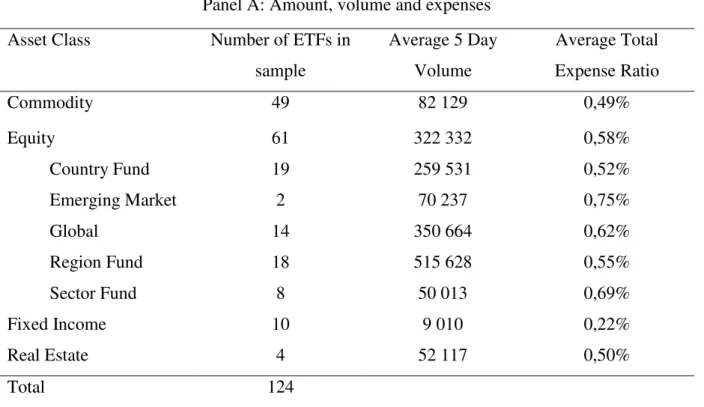
Table 1: Sample Characteristics Panel A: Amount, volume and expenses
Asset Class Number of ETFs in
sample
Average 5 Day Volume
Average Total Expense Ratio
Commodity 49 82 129 0,49%
Equity 61 322 332 0,58%
Country Fund 19 259 531 0,52%
Emerging Market 2 70 237 0,75%
Global 14 350 664 0,62%
Region Fund 18 515 628 0,55%
Sector Fund 8 50 013 0,69%
Fixed Income 10 9 010 0,22%
Real Estate 4 52 117 0,50%
Panel B: ETF Provider
ETF Provider Number of ETFs in sample Average Total Expense Ratio
ETFS 47 0,49%
iShares 50 0,48%
Lyxor 12 0,54%
Powershares 12 0,59%
SPA Marketgrader 3 0,85%
Equity funds are sorted on their Bloomberg classification. Average 5-day volume based on last 5 trading days: 21-05-14 to 27-05-14. Fund which were available on the LSE on 1-1-2008.
The final sample is displayed in table 1 whereas Appendix A shows the individual funds within the sample. Table 1 shows that there is a balanced selection of funds including domestic and internationally focused funds covering multiple asset classes. Equity, fixed income, commodities and real estate are all included in the sample. Furthermore, the equity funds have been divided in five market-based subcategories. Of the total of 124 funds, 61 funds are equity funds in which region, global and country funds seem to be the most popular ETF category both in number and in average trading volume. Only two funds are specific emerging market funds but among the country and region ETFs there are more funds which get exposure from developing markets. The eight sector funds complete the equity sample and represent the smallest group in average trading volume. Ten of the listed exchange-traded funds are fixed income funds and they all focus on the European or United States bond market. Finally, four real estate ETFs are offered on the exchange of which one is an emerging market real estate fund and the other three are real estate funds targeting some developed market.
and risks associated compared to futures contracts or compared to the physical commodity. Just like regular ETFs, ETCs trade exactly like stocks and are thus more intuitive and straightforward to understand than futures contracts. The LSE offers ETCs on individual commodities and on commodity indexes. Contrary to equity ETFs, where return comes from the change in price of the underlying stocks, ETCs have three sources of return. According to the London Stock Exchange (2009) the first source of return is the change in the price of the commodity futures contract, largely determined by changes in spot prices. The roll (down or up) is the second driver for return and refers to the rolling down of the futures contract from one month to the other as the earliest contract reaches expiration. Finally, the third source is the interest on collateral, which in this case means interest earned on the cash proportion of the initial investment.
When looking at panel B of Table 1 it becomes clear that there were only a few ETF issuers on the ETF market in the United Kingdom in 2008. 50 of the ETFs in the final sample are managed by iShares. iShares are a series of ETFs managed by BlackRock and are offered on many exchanges across the globe. Lyxor, part of Société Générale Group, and PowerShares, offered through Invesco, both have 12 ETFs listed in the exchange and included in the sample. SPA Marketgrader has three funds in the sample but all have been delisted in 2009. All the other funds are commodity funds and except for two delisted Lyxor funds, all of these exchange traded commodity funds are offered by ETFS. The fact that there is little competition in the ETF market on the LSE might have some effect on the performance and tracking error among the funds.
fees compared to the developed market funds. Emerging market equity funds charge an average of 0,75%, the highest among the equity funds. On average equity funds charge 0,58% with a maximum of 0,95% and charge at least 0,15%. Country equity funds have the lowest average cost among the equity funds. The fixed income or bond funds all have very low expense ratios with a minimum charge of 0,20% and a maximum charge of 0,25% resulting in an average of 0,22%. Finally, the real estate funds have moderate expenses: either 0,40% or 0,59% with an average at 0,50%.
Methodology
General Performance
General performance will be evaluated using the return of the ETFs, the standard deviation of the ETFs and the information ratio in order to get a risk-return relationship. Logarithmic returns are used to calculate the return of the ETF and the index. More specifically, the return of the ETF is determined using the following equation:
where Retf,t is the daily return of the ETF, Petf,t is the closing price at t and Petf,t-1 is the closing price of the day before. The standard deviation of the returns for each ETF is calculated as follows:
Where SD is the standard deviation of the returns, Retf,t the return of the ETF at time t,
the mean return of the ETF and n the amount of observations.
To get a better idea of the risk and return relationship, the information ratio is calculated. Combining the volatility and the return of a security allows for the determination of the Information Ratio. This ratio is defined as:
converted to yearly figures in order to estimate the information ratio. When converting the daily return to a yearly figure the return is simply multiplied by the amount of trading days in a year. In this study, a year is assumed to contain 250 trading days for the United Kingdom. The daily standard deviation is converted to a yearly figure by multiplying it by the square root of 250 (15,81). The information rate gives an indication on the risk-adjusted return of the ETF or index and indicates the extent to which risk taking is compensated by a higher return.
The general performance section will also include a correlation analysis between the return of the ETFs and the return of the benchmark indices. The correlation matrix will show whether index return variation is replicated by the exchange-traded funds or not. The correlation analysis will be done on an asset class level for the whole time period. The correlation coefficient is calculated as follows:
where is the correlation coefficient, the covariance between the return of
the benchmark index and the return of the ETF, and and are the variance of the index return and the ETF return respectively.
ETF discount and premium
There can be a difference between the price of the ETF on the market and the net asset value (NAV) of the fund. The net asset value represents the intrinsic value of the ETF or the value of the investments held by the fund, which underlies the creation and redemption. If the price of the ETF is above the NAV there is a premium, if the price is less than the NAV there is a discount. Following Engle (2006) and similar to Jares (2004), the premium is defined as followed:
In which pt is the price of the ETF at time t and nt the net asset value of the ETF at time t. The use of log differences is preferred over simple differences due to the big price differences within the sample of ETFs and naturally bigger premiums or discounts for expensive funds.
Tracking Error
used the price of the ETF in order to calculate the return. Others used the NAV of the ETF in order to calculate the returns. This study is going to use the closing prices of each fund and not the NAV. Ultimately the investor cares about the price she can buy or sell the fund at. The NAV is important to consider but will not be the focus and thus tracking error will be based on the price instead of the NAV from now on. Even if the NAV was used instead of price, it is not expected that it would yield very different results due to the creation and redemption process which generally keeps prices and NAV very close.
A range of methods has been used to determine the tracking error in previous research. Aroskar and Ogden (2012) summarised five methods in order to calculate the tracking error. Despite the fact that Aroskar and Ogden used a sample of ETNs instead of ETFs, the same tracking error formulas can be used. The methodology and intuition behind the tracking error of ETNs is identical to ETFs and thus these five methods can be replicated in this study without any further adjustments. Each of these five methods will be discussed and explained in this section. Each method will be used later on to calculate the tracking error of the ETFs in the UK sample.
According to Aroskar and Ogden (2012), Wong and Shum (2010) offer the first and most straightforward method to calculate the tracking error of ETFs. They define the tracking error simply as the difference between the daily return of the ETF and the daily return of the underlying index:
Logarithmic returns are used to calculate the return of the ETF and the index. The logarithmic return of an ETF is calculated using formula (1), which has already been specified previously. The return of the index is calculated in an identical way:
where RI,t is the daily return of the underlying index, It is the index value at t and It-1 is the
different methods or not. Nevertheless it is a good start to find out if there is some degree of tracking error in the funds or not.
The second method to determine the tracking error comes from a study by Gallagher and Segara (2005). This method uses the absolute difference between the returns instead of the simple difference. This way, both negative and positive returns are treated the same. An investor with a long position will surely not complain if the ETF will perform slightly better than the index but the ETF is created to track its index as accurate as possible. Hence it is fair to treat positive and negative returns the same since the most accurate tracking is generally desired and is the aim of this investment product. This second measure of the tracking error should thus be more informative than the first method and by definition show a tracking error which is at least as high as the tracking error found using the first method. The second method, the daily average absolute tracking error, is calculated as follows:
Where n is the amount of observations and e is defined as the simple difference between the return of the ETF and the index:
The third method for estimating the tracking error is the standard deviation of the difference in returns between the exchange-traded funds and the underlying index. Following again Gallagher and Segara (2005) the standard deviation of the difference is calculated using the following equation:
one or more of the other methods to get a more reliable picture. When the standard error of difference indicates a tracking error and this is confirmed by other methods it is most likely an accurate measure.
The final two methods for determining the tracking error use the standard linear regression model defined as follows:
The fourth method (TE 4) comes from Aroskar et al. (2012) who argue that the R-squared of the previously mentioned regression equation (11) is another indicator for the tracking ability of an exchange-traded fund. The R-squared is particularly advantageous because it is a statistic that is very intuitive and easy to interpret. It shows how much of the variation in the ETF price is explained by variation in the price of the underlying index. The R-squared of regression model (11) will thus be used as the fourth method of tracking ability estimation.
The fifth and final method (TE 5) comes from Chu (2011) who uses the standard error of regression (11) as a method to determine the tracking error. The standard error of a regression can be seen as the average distance of all of the observed data points and the estimated regression line. It is important to note however that this method only gives a good approximation to the tracking error in case the β-coefficient is equal to 1. If the β-coefficient is not equal to 1, the tracking error may be overstated according to Pope and Yadav (1994).
Correlations
In which is the correlation coefficient, is the covariance between the tracking error and the V2X index and and the variance of the tracking error and the V2X index respectively. By substituting V2X for the VIX or the credit spread in the covariance and the second variance variable, the correlation between the tracking error and the VIX or the credit spread will be calculated. If the correlation coefficient (r) is significantly above 0 the volatility of the market increases the tracking error of the ETFs. The closer the coefficient is to 1 the stronger the relation between the 2 variables. If the coefficient is 0 or insignificant there is no evidence of a relation between the two factors. If the coefficient is negative, market volatility would improve tracking ability of the funds, this is not expected. It is expected that the coefficient r will be positive for all of the volatility versus tracking error correlations.
Determinants of the Tracking Error
After establishing whether a fund shows some tracking error an attempt is made to find out what the determinants are of the tracking error. Frino and Gallagher (2001) have established that lower expense ratios (EXP) result in a lower tracking error. Chu (2011) also finds that the fees charged by an ETF have a significant effect on the tracking error but the direction of the effect is contradicting. Using the R-squared method for the tracking error Chu found that the effect of fees was slightly negative on tracking error, but using 3 other methods for the tracking error the effect of fees was significantly positive. Given that funds may charge investors for the operational costs of managing the fund, ETFs with lower rebalancing needs and thus lower costs perform better (Aroskar and Ogden, 2012). As indicated before, total expense ratios are a yearly figure and range from 0,15% to 0,95%. Furthermore, it is assumed that for each fund the total expense ratio has not changed during the time period studied and thus the total expense ratio is assumed to be constant.
the standard deviation of the returns and included in the regression model as the second independent variable (RISK).
The size of a fund, measured by the assets under management, has been found to be a potential source of the tracking error. Chu (2011) and Drenovak et al. (2012) find that the size of a fund can have a significant negative impact on the tracking error indicating that big funds do better in tracking their benchmark than small funds. Better tracking performance by large funds can be the result of several things. High assets under management (size) mean that investors have trusted high amounts of capital to the fund and thus the fund manager may feel more pressure to perform well. Next to that, Perhaps larger funds are able to attract better fund managers and skilful employees who allow for improved tracking performance. Finally, large funds might have economies of scale when trading which could improve their performance. In order to find out whether size has an impact on the tracking error for the UK funds, their average assets under management is calculated and will represent the third variable (SIZE).
A volatility factor that represents the daily price volatility of the ETF will be the fourth and final independent variable (dVOL) in the regression model. Intra-day price volatility is also expected to capture some effect from the liquidity of a fund. It is expected that if daily price volatility is high there are relatively many trades, indicating that the fund is active and that there are no liquidity issues. According to Shin and Soydemir (2010) the volatility of the ETF intra-day price has a positive impact on the tracking error. The daily price volatility will be approximated using the high, low and close price of the security. More specifically, the average volatility of the daily price is equal to:
where Pt,high is the daily high of the ETF on day t, Pt,low is the daily high of the ETF on day t and Pt,close is the closing price of the ETF at the end of day t. It is expected that only the most traded funds will really show any daily price volatility.
This gives the following cross-sectional regression model:
TEi,t= β0+ β1*EXPi+ β2*RISKi + β3*SIZEi,+ β4*dVOLi+ εi (13)
return differences (TE 3) and the standard error of the regression model (11) (TE 5) are all used in order to get the most consistent results. The simple tracking error and the R-squared are not used as they seem of lower quality than the other three methods.
Results
Results will be discussed on an asset class level and to a lesser extent on a fund level. If specific funds are discussed, their Bloomberg ticker will be used as an identifier. In order to see if there are developments over time, sub-periods are created. Most results will be presented over the full time period, six yearly time periods (2008 until 2013) and two crisis periods. The crisis periods will be addressed separately as they may be particularly interesting and give an idea about performance and tracking ability during economic crisis periods and volatile markets. The crisis periods are defined as follows: first is the 2008 financial crisis (FC) period that lasted from April 2008 until September 2009 (six quarters). This is based on the quarters that the United Kingdom’s economy was in a recession. According to the organisation for economic co-operation and development (OECD), the UK experienced a quarter-to-quarter GDP growth of -0,9, -1,4, -2,1, -2,5 -0,4 and 0,0 from 2008 Q2 to 2009 Q3 respectively. The second crisis period is the European sovereign debt crisis (DC) that lasted for three quarters from October 2011 until June 2012. According to UK recession figures from the OECD, the GDP growth during this period was -0,1, 0 and -0,4 (2011 Q4 - 2012 Q2). The first economic crisis (FC) period lasts twice as long and was a lot more severe then the most recent debt crisis when comparing the GDP growth figures. Nevertheless, both crises periods are associated with increased market volatility according to implied volatility indices and are thus particularly interesting to analyse separately. By creating these crisis sub-periods it is possible to see whether exchange-traded funds performed differently during any of the crisis periods compared to non-crisis economic periods.