- 0 -
A Work Project, presented as part of the requirements for the Award of a Masters
Degree in Economics from the NOVA – School of Business and Economics.
CORRELATES OF INTERGENERATIONAL MOBILITY AND POLITICAL
VIOLENCE
MATILDE POLÓNIA GONÇALVES GRÁCIO
684
Supervision of:
Professor Pedro Vicente
- 1 - Correlates of Intergenerational Mobility and Political Violence1
Abstract
This work project aims at exploring the role of intergenerational immobility in
political violence. A cross-country macro-level analysis is done where no significant
results are found. Additionally, an individual micro-level analysis is done where
intergenerational mobility (measured through a proxy variable) has a negative
significant effect in political violence.
Keywords: Intergenerational Mobility, Political Violence
1. Introduction
According to the Armed Conflict Report 20142, between the 1st of January and the 31st of December of 2013 there were 28 active armed conflicts in 25 countries; with Africa hosting 12 of these conflicts. Because conflict persists so should the work to
understand it. Therefore, this work project contributes to the literature on the correlates
of political violence. In detail, it focuses its efforts in entering the debate of the different
measures of societal inequality as a source – or at least a correlate – of political
violence. The aim of this work project is to access the role played by intergenerational
immobility in explaining political violence.
In order to answer this question two separate approaches are followed. The first
entails a macro-level analysis of the relationship between intergenerational immobility
and political violence. To do so, I first construct the measure of intergenerational
immobility using a highly adopted method in the intergenerational mobility literature –
the two-sample two-stage least squares estimator. Then I use this estimated measure of
- 2 -
mobility to test for the relationship between intergenerational mobility and political
violence. Notice that in order to obtain robustness in the results several extensive
margin and intensive measures of political violence were used. The second approach
entails a micro-level individual analysis. This uses a proxy measure of intergenerational
mobility and relies on survey self-reported measures of well-being and use of violence
due to political reasons. More specifically, in this section I test if the difference in
well-being of an individual compared to its parents 10 years ago (proxy measure of
intergenerational mobility) has an effect on individual use of political violence.
Additionally, I look at the impact in political violence of the different movements of the
standings in well-being, i.e. i) an upward movement (where an individual is better-off
than his parents), ii) no movement (where an individual is in the same stand as his
parents) and, iii) downward movement (where an individual is worse-off than his
parents).
Results of the several estimations done go as follows. For the first (macro-level)
approach, I find no significant effects of the main variable of interest in political
violence. I find however some significant results on variables such as GPD per capita,
degree of freedom of a country and amount of urban population (in line with the
literature). For the second approach (micro-level) I find that the proxy measure of
mobility yields significant negative effects in political violence.
The rest of the work project will develop as follows. Section 2 provides a concise
literature review of the topic. Section 3 contains a theoretical framework. Section 4
focuses on the empirical results, and it is divided into data description, estimation
- 3 -
2. Literature Review
Interest in the causes of conflict is as old as Plato and Aristotle. The later rooted
civil unrest within the Athenian society in three fundamental causes: “i) the unequal
nature of Athenian society, ii) frustration with the weakness and incompetence of
Athens’ leaders and iii) the desire for the wealth and privilege that holding political
office may entail” (Jacoby, 2008, p.10). All three ideas have been explored by
economics using different datasets and methodologies with the intent to explain political
violence or, more frequently, the starkest manifestation of such violence: civil war.
Seminal work by Collier and Hoeffler (1998; 2004) shows that greed rather than
grievance explains rebellion. They find that economic factors, particularly the ability to
finance and organize a rebellion (captured by the existence of natural resources, as well
as economic growth and male secondary education enrollment) strongly predict the
outbreak of a civil war. Fearon and Laitin (2003) conclude that proxies for political
grievances such as ethnic and religious diversity have little explanatory power in
predicting the onset of a civil war. Additionally, proxies for state institutional capacity
and strength (most importantly measured by per capita income) are considered robust
predictors of civil war. Montlavo and Reynal-Querol (2005) who study the relationship
between conflict and ethnic polarization (introduced in the theoretical work of Esteban
and Ray, 1994, 1999) provide significant support for “deep cleavages” along large
group lines to affect conflict. Esteban, Mayoral and Ray (2012) draw from the
theoretical work of Esteban and Ray (2011) to study the impact of ethnic divisions on
conflict. More specifically, they look at polarization, fractionalization and the
Gini-Greenberg index, and link them to conflict intensity finding significant evidence that
- 4 -
an overview of other explanatory variables that have been considered as correlates of
conflict such as population, geographical and environmental variables.
Inequality has been highly disregarded as a consistent way to explain conflict.
Despite the great amount of approaches undertaken in order to identify the role of
inequality in political violence, it is not clear that inequality (traditionally measured by
the Gini index) has a correlation with conflict. Explanations in the literature for the
non-existence of this relation draw for reasons such as the lack of good measurement and
availability of data for inequality. Moreover discussions on the explanatory power of
different types of inequality, e.g. vertical inequality, horizontal inequality, inequality
within the same group, for political violence seem to play an important role. It is within
this context that the measurement of intergenerational mobility, i.e., the way that
inequality persists across generations, plays in the incidence and magnitude of political
violence.
3. Theory
The theoretical framework used follows a very simplistic approach to the extensive
work of Besley and Persson (2011). Although the aim of the empirical part of this work
is not directly related to the model it is still a good framework to understand
mechanisms of inequality in explaining political violence.
Let’s consider a two period model s = 1, 2 and two groups of individuals (A, B),
with half the population each. In the beginning of the first period one of the groups
holds power (incumbent) I1 ∈ {A, B}, the other group is opposition O1 ∈ {A, B}. γ, is a
measure of political instability. More specifically, it is the outcome of a potential
conflict that is triggered by investments in violence by the incumbent and the
- 5 -
The utility function of an individual is given by usJ = csJ+ αsgs, where private
consumption csJ depends on the net tax income (1 − ts)y(p𝑠𝐽) and transfer received rsJ.
gs is a public good (and here we assume a linear relation). And αs has a two-point
distribution αs ∈ {𝛼𝐿, 𝛼𝐻}, where 𝛼𝐻 > 2 > 𝛼𝐿 > 1 and Prob[αs = αH] = ∅. The
income tax is constrained by existing fiscal capacity (ts < 𝜏𝑠). y(. ) is and increasing
concave function. y(p𝑠𝐽) is wages or ownership of other factors such as land or capital.
Government budget constraint at date s is given by: 𝑅 + ts𝑦(𝑝𝑠𝐼)+𝑦(𝑝𝑠𝑂)
2 = 𝑔𝑠+ 𝑚𝑠+
𝑟𝑠𝐼+𝑟𝑠𝑂
2 , where 𝑅 is time-independent revenue source accruing only to government and
𝑚𝑠 = ℱ(𝜏2− 𝜏1) + ℒ(π2− π1) + 𝜔(π1)𝐿𝐼 if 𝑠 = 1 and 0 if 𝑠 = 2 is the investment
cost in fiscal capacity. Constraints in the incumbents allocation of transfers is given by
𝜃 =1+𝜎𝜎 ∈ [0,12]; the incumbent must give a fixed share 𝜎 to the opposition for any unit
of transfers awarded to its own group.
The timing of events is the following:
1. We begin with initial stock of state capacities {𝜏1, 𝜋1} and an incumbent group
𝐼1. Nature determines 𝛼1and R.
2. 𝐼1chooses a set of period-1 policies {g1, t1, p1I, p1O, r1I, r1O} and determines through
investments the period-2 stocks of fiscal and legal capacity {𝜏2, 𝜋2}. 𝐼1 and 𝑂1
simultaneously invest in violence levels 𝐿𝐼 and 𝐿𝑂.
3. 𝐼1 remains in power with probability 1- γ(Lo, LI,), and nature determines 𝛼2.
4. 𝐼2 chooses period-2 policies {g2, t2, p2I, p2O, r2I, r2O}.
The incumbent chooses the optimal policy vector {gs, ts, psI, psO, rsI, rsO} so as to
maximize αsgs+ (1 − ts)y(psI) + rsI. Subject to ts ≤ τs, psI ≤ πs, and rsO ≥ σrsI and the
- 6 -
maximize the expected utility period-2 utility of group J in period 1: W(α1, τ1, m1, βJ) +
(1 − γ(Lo, LI,))UI(τ
2, π2) + γ(Lo, LI,)UO(τ2, π2) for the incumbent group, and
W(α1, τ1, m1, βJ) −ω(π1)LO+ γ(Lo, LI,)UI(τ2, π2) + (1 − γ(Lo, LI,))UO(τ2, π2)
for the opposition group. 𝜔(𝜋1)𝐿𝑂, is the private cost of violence and needs to be
deducted for the opposition group. The incumbent uses public funds.
Inequality is one of the extensions introduced in the model and it is constructed by
considering differences in wages between the incumbent and the opposition groups with
ωJ for J ∈ {I, O}. Let there be two levels of wages ωJ∈ {ωL, ωH}. Let ω denote the
average wage ω = (ωH+ ωL)/2.
The authors present some predictions of the introduction of inequality in the model,
which I translate here. If the incumbent is poor it will lead to a higher investment in
state capacity. On the other hand, if the incumbent is rich it will diminish the investment
on fiscal capacity. Additionally, some discussion is also introduced on the effect of
inequality in investments in political violence. According to the authors, an asymmetry
in wages might make the richest group less inclined to violence. This can be called a
“loyalty premium”, where the high income group would recruit people from its own
ranks increasing the cost of violence. However, rich and violence-prone groups would
wish to hire low-wage individuals to carry out violence on their behalf. Moreover, one
group could be better organized in raising resources for fighting when in opposition,
i.e., lowering the costs of violence, making political violence more likely.
4. Empirical Results
4.1. Data
Demographic and Health Surveys (DHS) – The DHS Program is a household survey
conducted consistently and periodically across different countries since 1984, providing
- 7 -
however due to data fit and availability, only phases two through five are used
(1991-2013)3. The structure of the dataset allows for the collection of information on an
individual’s wealth and characteristics provided he is the head of the household, as well
as individual characteristics of other members of the household. More specifically,
information collected on the individuals’ wealth is constituted by household
characteristics and ownership of goods4. The relevant individual characteristics
provided for both head of household and other members of the household are age,
education, and type of location of residence (urban or rural)5. This dataset allows for the
estimation of intergenerational mobility6.
Center for Systemic Peace, Major Episode of Political Violence (MEPV) –A MEPV
is defined “by the systematic and sustained use of lethal violence by organized groups
that result in at least 500 directly-related deaths over the course of the episode”7. The
MEPV dataset contains information from 1946 until 2014 on magnitude scores of
MEPV for all countries. The information contained in this dataset is transformed into a
dummy variable that reports simply the existence or not of a MEPV by country and
year.
Armed Conflict Location and Event Data Project (ACLED) – The ACLED is a
comprehensive dataset on political violence for developing states. The latest version
(Version 5) is used and includes data from 1997 until 2014. The ACLED main focus is
on politically violent events, which are defined as “a single altercation where often force
3 First-round of surveys did not include the questions that provided the required information. Sixth and
seventh rounds are not yet complete and/or available for every country.
4 Household characteristics and ownership of goods: source of drinking water, location of water source,
toilet facilities, material of construction of the roof-top, number of rooms in the household per person, electricity, radio, television, mobile-phone, refrigerator, bicycle, motorcycle and car.
5 To avoid different cultural settings for women across countries, only men are considered.
6 Countries for which this dataset is complete and available are: Ghana, Kenya, Malawi, Mali, Mozambique, Namibia, Nigeria, Senegal, Tanzania, Uganda and Zambia
- 8 -
is used by one or more groups for a political end (…)”8 .The dataset contains
information on dates and locations of political violence as well as estimated reported
fatalities per event of political violence.
Afrobarometer – The Afrobarometer dataset provides micro-level information on
“…the social, political, and economic atmosphere in Africa”9. Round two (2004) of the
Afrobarometer dataset is used10. More specifically, the information is provided by the
following questions: i) “on a scale between 0 and 10, where 0 are “poor” people and 10
are “rich” people: Which number would you give your parents ten years ago?”, ii) “on a
scale between 0 and 10, where 0 are “poor” people and 10 are “rich” people: Which
number would you give yourself today?”, and iii) “… please tell me whether you,
personally, have done any of these things during the past year. If not, would you do this
if you had the chance: Used force or violence for a political cause?” The first two
questions provide a way to estimate a proxy for intergenerational mobility. The third
question provides information on self-reported use of violence due to political reasons11.
Other datasets – The Word Development Indicators (WDI) dataset is used to obtain
information on i) Gini Coefficient, ii) GDP per capita and iii) Urban Population. Fearon
and Laitin (2003) is used to obtain data on percent of mountainous terrain. Information
on the degree of freedom of a country is taken from the Freedom House dataset.
Measures of Ethnic Fractionalization and Ethnic Polarization are taken from Montlavo
and Reynal-Querol (2005).
8 For more information see:
http://www.acleddata.com/wp-content/uploads/2015/01/ACLED_Codebook_2015.pdf (page 7) 9For more information see: http://www.afrobarometer.org/
10 To avoid different cultural settings for women only men are considered.
- 9 -
4.2. Estimation Strategy
In order to analyze the relation between intergenerational immobility and
political violence two different approaches are established. The first uses macro-level
data and entails first, the construction of a measure of intergenerational immobility.
This allows cross-country analysis of intergenerational immobility and political
violence. The second uses micro-level data, individual level analysis of
intergenerational mobility and political violence.
This section is therefore divided in three parts. The first provides the estimation
strategy for the construction of the variable of intergenerational immobility. The second
demonstrates the specifications used to obtain a macro-level relation between
intergenerational immobility (using the measure obtained in the first stage) and political
violence. The third provides the estimation strategy for a micro-level analysis of
intergenerational mobility and political violence.
4.2.1. Measurement of Intergenerational Immobility
The measurement of intergenerational immobility is often done through
intergenerational elasticity (IGE) which is provided by the following equation:
Yi = β0+ β1Ypi+ εi (1)
where Yi is life-time earnings of the children, Ypi is life-time earnings of parents, β0 is a
constant, εi is the error term and β1 is the measure of intergenerational immobility
(IGE). When β1 is zero, life-time earnings of the children do not depend on the parents’
life-time earnings (full mobility); when β1 is one, life-time earnings of the children
depend fully on the life-time earnings of the parents (no mobility).
Recurrent issues in the intergenerational mobility literature related with data
availability and fitness of survey method impede the estimation to be done as described
- 10 -
Angrist and Krueger (1992) is a broadly accepted method that mitigates data restriction
issues. More specifically, this project uses the two-sample two-stage least squares
estimator (TS2SLS) first used by Björklund and Jäntti (1997) to estimate
intergenerational mobility, that was massively adopted in the intergenerational mobility
literature. This method is asymptotically more efficient (Inoue and Solon, 2010), and
computationally easier than TSIV. The TS2SLS estimation relies on two distinct
samples. A sample of individuals (secondary sample) that constitute a set of
pseudo-parents, used to predict life-time earnings of an individual with a given set of
characteristics. A second sample of individuals (main sample) that constitute the
children that report on their own earnings and characteristics, as well as their parents’
characteristics.
Provided the structure and content of the DHS dataset the two samples for the
estimation of intergenerational mobility through TS2SLS are obtained by splitting the
overall sample into two. The secondary sample is constituted by male individuals born
before 1960 that are heads of household (pseudo-father). The main sample is constituted
by male individuals born after 1960 that are heads of household and whose father lives
in the household (son). The wealth of the individual is used as a proxy for his life-time
earnings.
Equations 2, 3, and 4 are the sequence of specifications that allow for estimation
of intergenerational immobility (IGE). LetWfj, be wealth of an individual in the
secondary sample. Let Ŵ fi be the predicted wealth of the father of the individual in the
main sample. LetWsi be wealth of an individual in the main sample. Let Xfjand Xfi be
a vector of characteristics, namely age, education and a dummy for urban location of the
household of an individual.
- 11 -
Ŵ fi = γ1Xfi (3)
Wsi = β0+ β1Ŵ fi+ εi (4)
β1is the estimated measure of intergenerational association of wealth between sons and
fathers; when equal to zero it means full mobility, and when equal to one it means there
is no mobility.β1 (IGE) is the value that is used in the next stage.
4.2.2. Intergenerational Immobility and Political Violence
The macro-level relationship between intergenerational immobility and political
violence is captured using extensive and intensive measures of political violence as
described below. Let the following equation (5) be the baseline for the several
estimations done.
Political Violencect = δ0+ δ1IGEct+ δ2Xct+ δ3Xc+ εct (5)
As previously mentioned two types of measures of political violence are considered.
The first type (an extensive measure), focuses on the existence of i) a MEPV (1 if there
is a major episode of political violence, and 0 otherwise) by country and year and ii)
existence of deaths (1 if there is at least one reported death, and 0 otherwise), provided a
politically violent occurrence has been registered, by country and year. We therefore
estimate the coefficients through maximum likelihood with a logistic specification. The
second type of measure of political violence tries to capture the intensity (magnitude) of
political violence. Thus, it uses intensive measures of political violence. The first being
the number of politically violent events registered by country and year and the second
being the number of deaths, provided a politically violent event was registered, by
country and year. The estimation of the coefficients is done using ordinary least squares.
The right side of the equation is similar in all specifications. δ0 is a constant. IGEct
- 12 -
year. X𝑐𝑡 is a vector, per year and country, of characteristics. X𝑐 is a vector of country
characteristics. 𝜀𝑐𝑡, is an error term.
4.2.3. Intergenerational Mobility Proxy and Political Violence
The relationship between self-reported perceived intergenerational mobility and
self-reported use of violent behavior due to political reasons is estimated in this section.
The micro-level relationship between intergenerational mobility and political violence is
given by the following equation:
Individual Political Violencei= δ0+ δ1IGE Proxyi+ δ2Xi+ δ3Xl+ εi (6)
where Individual Political Violencei is an ordered categorical variable of self-reported
use of violence due to political reasons (0=No, would never do this, 1=No, but would do
if had the chance, 2=Yes, once or twice, 3=Yes, several times, 4=Yes, often).
IGE Proxyi is the difference between self-reported current well-being of an individual
and the well-being of its parents 10 years ago (integer scale between -10 and 10; -10=an
individual is 10 times worse than its parents, 0=an individual has the same well-being as
his parents, 10=an individual is 10 times better than his parents). Xi is a vector of
individual characteristics12 and Xl is a vector of location controls13.
Issues of endogeneity do not go unnoticed throughout the work. Indeed one
might argue that reasons that explain the difference in well-being between individuals
and parents might be the same that explain the engagement in political violence. One
common approach to deal with issues of endogeneity is to introduce an instrumental
variable (IV). The basic idea behind the use of an IV is to find a variable that explains
12 Individual control variables: age, head of household dummy, urban dummy, no schooling (base category), complete primary schooling, complete secondary schooling, higher education, no employment (base category), part time employment, full time employment, income (first quintile), income (second quintile), income (third quintile) (base category), income (fourth quintile), income (fifth quintile).
- 13 -
the dependent variable only through its effect in the independent variable. In detail the
necessary conditions to use an IV are the following:
Cov(𝑍, x) ≠ 0 (7)
Cov(𝑍, ε) = 0 (8)
Equation 7, states that the instrument (Z) must be correlated with the endogenous
explanatory variable. Equation 8, also known as the exclusion restriction, states that the
instrument (Z) must be exogenous, i.e., it must be uncorrelated with any other
determinants of the dependent variable.
In this specific context, we want to explain the use of violence due to political
reasons trough a variable that is only related to the difference in well-being between
individuals and their parents. A thorough exploration of the dataset available led me to
believe that a measure of availability of goods14 might work as a good IV provided a
good control of an array of other variables. The main idea behind the use of this IV, is
that provided the extensive use of control variables that influence the well-being of an
individual, the availability of goods might be linked to political violence solely through
the difference in well-being between individuals and their parents. Therefore the
first-stage regression (equation 9) and then the reduced form (equation 10) are estimated:
IGE Proxyi = ϑ0 + ϑ1Zi+ ϑ2Xi+ ϑ3Xl+ ωi (9)
Individual Political Violencei= δ0+ δ1Zi+ δ2Xi+ δ3Xl+ εi (10)
where Zi is as ordered categorical variable of the availability of goods compared to the
past (1= Much Worse, 2=Worse, 3=About the Same, 4=Better, 5=Much Better). All
other variables are equal to equation 6.
14 The specific survey question and possible answers are the following:
Please tell me if the following things are worse or better now than they used to be, or about the same: The availability of goods?
- 14 -
Throughout this project one main assumption that has been in place is that
mobility (or immobility) has the same impact on political violence whether it allows for
an individual to improve his life easily (upward mobility) or to worsen his life easily
(downward mobility). In order to try to understand the differences of the effect of the
two movements on political violence we replace the previous proxy variable of
intergenerational mobility with a categorical variable that comprises the three types of
movements that are observed when comparing an individual’s well-being with his
parents well-being 10 years ago (worse – or downward mobility, equal – or no mobility,
and better – or upward mobility). The estimation follows the equation:
Individual Political Violencei= δ0+ C1IGE Proxy𝑖 + δ2Xi+ δ3Xl+ εi 15(11)
IGE Proxy𝑖 is therefore a three category variable of the difference between the current
well-being of an individual and the well-being of its parents 10 years ago; base category
is Downward Mobility (negative difference), No Mobility (no difference) and Upward
Mobility (positive difference). All other variables are the same as in equation 6.
4.3. Results
4.3.1. Measurement of Intergenerational Mobility
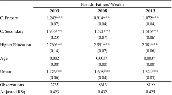
Table 1 provides an example of first-step estimation by Ordinary Least Squares
for the estimation of IGE. Level of education and urban/rural location are persistently
significant at 1% level across the specifications of the three years (2003, 2008, and
2013). Having complete primary or secondary or higher education studies increases the
level of wealth, on average, ceteris paribus, compared to the base category (no
education). Living in an urban region increases wealth of an individual, on average,
ceteris paribus. Age of an individual is significant at a 10% level in 2008 and 2013 and
it has a positive effect.
- 15 -
Table 2 provides the second stage regression. The predicted fathers’ wealth is
significant in all specifications. Having complete secondary level of schooling or above
is also significant in 2008 and 2013. However, despite the significance in this specific
country of some levels of education in determining wealth of an individual, the IGE
estimates that are considered for the next stages of the project are in columns 116. Table
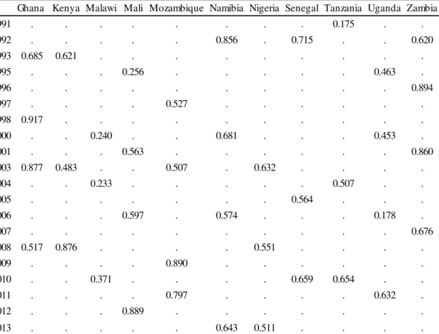
3 provides a summary of all (country and year) IGE estimates.
16 Including the measure of IGE that also takes into account the levels of education of an individual is difficult in the context of a cross-country analysis where levels and degree of importance attributed to education are different across countries.
Table 1: First-Step Estimation (Nigeria)
2003 2008 2013
C. Primary 1.242*** 0.914*** 1.072***
(0.07) (0.04) (0.04)
C. Secondary 1.936*** 1.521*** 1.616***
(0.23) (0.07) (0.06)
Higher Education 2.760*** 2.551*** 2.381***
(0.14) (0.07) (0.06)
Age 0.002 0.003* 0.003*
(0.00) (0.00) (0.00)
Urban 1.476*** 1.698*** 1.324***
(0.06) (0.04) (0.03)
Observations 2735 8613 8199
Adjusted RSq 0.423 0.432 0.425
Pseudo-Fathers' Wealth
- 16 -
Table 2: IGE Estimation (Nigeria)
(1) (2) (3) (1) (2) (3) (1) (2) (3)
P. Father Wealth 0.632*** 0.426* 0.451* 0.551*** 0.442*** 0.456*** 0.511*** 0.391*** 0.414***
[0.00] [0.52] [0.02] [0.00] [0.00] [0.00] [0.00] [0.00] [0.00]
C. Primary 0.075 0.084 0.018 0.033 0.100 0.099
[0.52] [0.47] [0.80] [0.64] [0.08] [0.11]
C. Secondary 0.045 0.042 0.259*** 0.267*** 0.149* 0.152*
[0.70] [0.73] [0.00] [0.00] [0.02] [0.02]
Higher Education 0.367 0.362 0.318*** 0.312*** 0.401*** 0.358***
[0.09] [0.09] [0.00] [0.00] [0.00] [0.00]
Age 0.107 0.103 0.174**
[0.29] [0.15] [0.01]
Observations 43 43 43 149 149 149 188 188 188
Adjusted RSq 0.385 0.423 0.420 0.299 0.410 0.417 0.257 0.364 0.389
2003 2008 2013
Sons' Wealth
- 17 -
4.3.2. Intergenerational Immobility and Political Violence
As mentioned in the previous section, two separate analysis of political violence
were implemented. The first takes into consideration two extensive margin measures of
political violence (the existence of a MEPV and the existence of casualties provided that
an event of political violence is registered). The second takes into consideration the
intensity of a political violent event by looking at the number of registered occurrences
per year and also at number of casualties per year (provided there was a political violent
conflict registered).
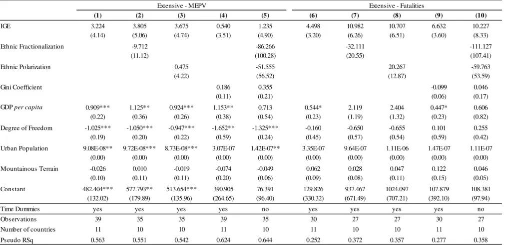
Table 4 reports results on the first approach taken. The signal is positive for
intergenerational immobility, i.e. has immobility increases the probability of both the
existence of a MEPV and the existence of at least one casualty provided there was a
politically violent event increase. The results are however not significant in all
Table 3: Summary Table of Estimated Intergenerational Elasticity (IGE)
Ghana Kenya Malawi Mali Mozambique Namibia Nigeria Senegal Tanzania Uganda Zambia
1991 . . . 0.175 . .
1992 . . . 0.856 . 0.715 . . 0.620
1993 0.685 0.621 . . . .
1995 . . . 0.256 . . . 0.463 .
1996 . . . 0.894
1997 . . . . 0.527 . . . .
1998 0.917 . . . .
2000 . . 0.240 . . 0.681 . . . 0.453 .
2001 . . . 0.563 . . . 0.860
2003 0.877 0.483 . . 0.507 . 0.632 . . . .
2004 . . 0.233 . . . 0.507 . .
2005 . . . 0.564 . . .
2006 . . . 0.597 . 0.574 . . . 0.178 .
2007 . . . 0.676
2008 0.517 0.876 . . . . 0.551 . . . .
2009 . . . . 0.890 . . . .
2010 . . 0.371 . . . . 0.659 0.654 . .
2011 . . . . 0.797 . . . . 0.632 .
2012 . . . 0.889 . . . .
2013 . . . 0.643 0.511 . . . .
- 18 -
specifications. Other measures of inequality are also not statistically significant across
any specification in neither measure of political violence. Some significant positive
effects are captured for GDP per capita, i.e., a higher GDP per capita increases the
probability of the existence a politically violent event; however results are not robust
across the two conflict datasets. The measure of the degree of freedom of a country is
also statistically significant across all specifications for the existence of a MEPV and it
holds the expected sign (more freedom, lower probability of a MEPV occurring). The
share of urban population has a significant (positive) effect on the existence of a MEPV.
Table 5 reports on the intensive measures of political violence. As can be observed.
IGE remains with a positive sign, although, still not statistically significant in either
variable. The only variable that captures persistent significant effects on the number of
politically violent events is the degree of freedom. It holds the expected value, more
freedom correlated to less reported occurrences of political violence. The share of urban
population holds significant results across the two variables in the specifications that do
not include time dummies: a higher amount of urban population increases both the
- 19 -
(1) (2) (3) (4) (5) (6) (7) (8) (9) (10)
IGE 3.224 3.805 3.675 0.540 1.235 4.498 10.982 10.707 6.632 10.227
(4.14) (5.06) (4.74) (3.51) (4.90) (3.20) (6.26) (6.51) (3.60) (8.33)
Ethnic Fractionalization -9.712 -86.266 -32.111 -111.127
(11.12) (100.28) (20.55) (107.41)
Ethnic Polarization 0.475 -51.555 20.267 -59.763
(4.22) (56.52) (12.87) (53.59)
Gini Coefficient 0.186 0.355 -0.099 0.046
(0.11) (0.21) (0.06) (0.17)
GDP per capita 0.909*** 1.125** 0.924*** 1.153** 0.713 0.544* 2.119 2.404 0.447* 0.606
(0.22) (0.36) (0.26) (0.38) (0.54) (0.23) (1.19) (1.32) (0.23) (0.82)
Degree of Freedom -1.025*** -1.050*** -0.947*** -1.652** -1.325*** -0.160 -0.650 -0.655 0.101 0.255
(0.19) (0.20) (0.22) (0.59) (0.24) (0.45) (0.57) (0.54) (0.59) (0.42)
Urban Population 9.08E-08** 9.72E-08*** 8.73E-08*** 3.07E-07 1.42E-07** 3.35E-07 9.64E-07 1.11E-06 1.47E-07 1.11E-07
(0.00) (0.00) (0.00) (0.00) (0.00) (0.00) (0.00) (0.00) (0.00) (0.00)
Mountainous Terrain -0.026 0.010 -0.019 -0.074 -0.049 0.062 0.028 0.047 0.122 0.046
(0.10) (0.11) (0.11) (0.20) (0.06) (0.09) (0.08) (0.11) (0.15) (0.05)
Constant 482.404*** 577.793** 513.654*** 390.905 76.391 129.826 937.467 1024.097 107.879 108.381
(132.02) (179.89) (135.96) (264.65) (96.40) (330.32) (671.49) (707.21) (392.10) (97.94)
Time Dummies yes yes yes yes no yes yes yes yes no
Observations 39 35 35 39 35 30 27 27 30 27
Number of countries 11 10 10 11 10 11 10 10 11 10
Pseudo RSq 0.563 0.551 0.542 0.624 0.644 0.252 0.372 0.357 0.277 0.358
Table 4: Extensive Political Violence and Intergenerational Mobility
Extensive - MEPV Extensive - Fatalities
- 20 - Table 5: Intensive Political Violence and Intergenerational Mobility
(1) (2) (3) (4) (5) (6) (7) (8) (9) (10)
IGE 125.943 200.730 184.204 164.301 167.034 749.142 1356.519 1218.729 1352.602 180.503
(191.06) (236.70) (230.73) (215.55) (196.01) (1257.89) (841.06) (812.51) (1362.15) (1248.23)
Ethnic Fractionalization -279.318 -4679.902 -554.357 -32142.44
(407.51) (2328.64) (3155.51) (15981.60)
Ethnic Polarization 122.692 -2596.751 -131.1583 -17879.71
(230.36) (1184.27) (2013.97) (7994.43)
Gini Coefficient -3.703 10.980 -58.265 58.181
(6.30) (7.20) (53.19) (46.89)
GDP per capita 11.264 34.529 32.546 6.568 21.374 26.535 156.134 124.550 -47.343 102.902
(18.57) (21.10) (21.67) (23.54) (18.84) (171.75) (171.24) (184.54) (190.27) (160.59)
Degree of Freedom -83.996* -81.929** -80.854** -84.408* -47.241 -671.76 -580.686 -570.915 -678.243* -358.729
(29.42) (18.58) (19.23) (28.43) (21.88) (327.91) (265.79) (184.54) (250.09) (191.49)
Urban Population 3.58E-06 -2.58E-06 -2.60E-06 3.04E-06 7.88E-06*** 0.0000512 2.77E-06 3.34E-06 4.27E-05 7.67E-05***
(0.00) (0.00) (0.00) (0.00) (0.00) (0.00) (0.00) (0.00) (0.00) (0.00)
Constant 239.8594 99.1899 -155.115 855.538 4603.913* 2696.325 -486.2375 -405.5217 8929.249 33262.82*
(258.02) (128.04) (551.86) (806.90) (1965.79) (2773.64) (1162.22) (3199.03) (6744.29) (13979.39)
Time Dummies yes yes yes yes no yes yes yes yes no
Observations 30 27 27 30 27 30 27 27 30 27
Number of countries 11 10 10 11 10 11 10 10 11 10
Adjusted RSq 0.471 0.886 0.882 0.441 0.539 0.547 0.897 0.897 0.570 0.580
Intensive – Number of Events Intensive – Fatalities
- 21 -
4.3.3. Intergenerational Mobility Proxy and Political Violence
This section shows the results for the estimations conducted with the
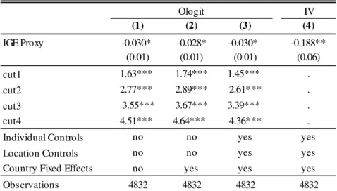
Afrobarometer dataset. Table 6 reports the results relative to equation 6.and equation
10. Table 7 reports the results relative to equation 11.
The coefficients of the proxy measure of intergenerational mobility hold
significant results (at 10%) across all specifications. The sign of the coefficients indicate
that if an individual perceives to be better off than its parents 10 years ago, the
probability of using violence due to political reasons reduces. The cut-offs are
statistically significant which indicates that the explanatory variable does not need to be
collapsed.
Table 6: Proxy Mobility and Political Violence
IV
(1) (2) (3) (4)
IGE Proxy -0.030* -0.028* -0.030* -0.188**
(0.01) (0.01) (0.01) (0.06)
cut1 1.63*** 1.74*** 1.45*** .
cut2 2.77*** 2.89*** 2.61*** .
cut3 3.55*** 3.67*** 3.39*** .
cut4 4.51*** 4.64*** 4.36*** .
Individual Controls no no yes yes
Location Controls no no yes yes
Country Fixed Effects no yes yes yes
Observations 4832 4832 4832 4832
Ologit
- 22 -
The results of the instrumental variable estimation also present a negative
significant relation between the self-reported measure of use of political violence and
the intergenerational difference in well-being17.
The results in Table 7 show the role of upward, non-existent and downward
mobility on the probability of an individual using violence due to political reasons.
Notice that across specifications 1, 3, and 5, having no mobility reduces significantly (at
a 10% level) political violence compared with the base category (downward mobility).
Additionally, in specifications 2, 4, and 6, in which the main objective was not only to
capture the effect of an upward or downward movement of intergenerational well-being
difference but also to understand if the current income position played any role, we
observe that measures of mobility have no significance. However, belonging to the fifth
quintile (as compared to the base category – third quintile) increases significantly (at
5% level) the probability of engaging in political violence. The interaction term between
having no mobility and belonging to the fifth quintile reduces significantly the
probability of an individual using violence due to political reasons. All cut-offs are
statistically significant which means that the categories on the explained variable do not
need to be collapsed.
- 23 - Table 7: Categorical Proxy Mobility and Political Violence
(1) (2) (3) (4) (5) (6)
No Mobility -0.247* -0.089 -0.227* -0.062 -0.219* -0.068
(0.11) (0.16) (0.11) (0.16) (0.11) (0.16)
Upward Mobility -0.164 -0.168 -0.169 -0.162 -0.171 -0.155
(0.09) (0.13) (0.09) (0.14) (0.09) (0.14)
Income (first quintile) -0.200 -0.148 -0.158
(0.17) (0.17) (0.17)
Income (second quintile) 0.228 0.238 0.233
(0.15) (0.15) (0.15)
Income (fourth quintilde) -0.042 -0.084 -0.046
(0.18) (0.19) (0.19)
Income (fifth quintilde) 0.597** 0.601** 0.633**
(0.22) (0.22) (0.23)
No Mobility * Income (first quintile) -0.027 0.012 0.035
(0.31) (0.31) (0.31)
No Mobility * Income (second quintile) -0.499 -0.501 -0.474
(0.30) (0.30) (0.30)
No Mobility * Income (fourth quintile) 0.150 0.079 0.102
(0.34) (0.34) (0.34)
No Mobility * Income (fifth quintile) -1.115* -1.200* -1.164*
(0.49) (0.50) (0.50)
Upward Mobility * Income (first quintile) 0.185 0.195 0.196
(0.27) (0.26) (0.27)
Upward Mobility * Income (second quintile) -0.268 -0.274 -0.263
(0.24) (0.24) (0.24)
Upward Mobility * Income (fourth quintile) 0.137 0.138 0.129
(0.26) (0.26) (0.26)
Upward Mobility * Income (fifth quintile) -0.159 -0.188 -0.162
(0.31) (0.31) (0.31)
cut1 1.51*** 1.56*** 1.62*** 1.71*** 1.33*** 1.38***
cut2 2.65*** 2.71*** 2.77*** 2.86*** 2.48*** 2.54***
cut3 3.43*** 3.48*** 3.55*** 3.64*** 3.27*** 3.32***
cut4 4.40*** 4.45*** 4.52*** 4.61*** 4.23*** 4.29***
Individual Controls no no no no yes yes
Location Controls no no no no yes yes
Country Fixed Effects no no yes yes yes yes
Observations 4832 4832 4832 4832 4832 4832
Note: Maximum Likelihood in an ordered logit specification. Explained variable, ordered categorical variable on self-reported use of violence due to political reasons (0=No, would never do this, 1=No, but would do if had the chance, 2=Yes, once or twice, 3=Yes, several times, 4=Yes, often). Explanatory variable a categorical variable of the difference between the current well-being of an individual and the well-being of its parents 10 years ago; base category is Downward Mobility (negative difference), No Mobility (no difference) and Upward Mobility (positive difference). Income (first quintile), dummy variable equal to 1 if individual belongs to the first quintile and 0 otherwise. Income (second quintile), dummy variable equal to 1 if individual belongs to the second quintile and 0 otherwise. Income (third quintile), dummy variable equal to 1 if individual belongs to the third quintile and 0 otherwise (base category). Income (fourth quintile), dummy variable equal to 1 if individual belongs to the fourth quintile and 0 otherwise. Income (fifth quintile), dummy variable equal to 1 if individual belongs to the fifth quintile and 0 otherwise. Interaction terms are represented by‘*’.
- 24 -
5. Conclusion
This work project had as its main objective to introduce intergenerational mobility
has a source of political violence. To do so, two separate approaches were undertaken.
The first relied on macro-level data to do a cross-country analysis. No significant effects
were found on the measure of intergenerational mobility in explaining political
violence. Some significant results on variables such as GPD per capita, degree of
freedom of a country and amount of urban population (in line with the literature) when
taking into consideration the existence of a MEPV. The second approach used
micro-level data to construct a proxy measure of IGE. I find that a higher positive difference in
well-being of an individual as compared to its parents ten years ago reduces
significantly the probability of the use of violence due to political reasons.
There are several fronts in which this field of research might benefit from future
work. The first is the development of a theoretical model that introduces not only
inequality, but also mobility of individuals in explaining political violence. Moreover,
mechanisms that lead to political violence should be further investigated. The second is
data availability and fitness to be able to better improve empirical estimations. The third
is to further explore micro-level mechanisms in understanding engagement in political
violence.
6. Bibliography
Angrist J.D., Krueger A.B. (1992), The effect of age at school entry on education attainment: an application of instrumental variables with moments from two samples, Journal of the American Statistical Association, 87, 328-336
Besley, Timothy, and Torsten Persson. 2011. Pillars of Prosperity: the political economics of development clusters. New Jersey: Princeton University Press.
- 25 -
Blattman, Christopher, and Edward Miguel. 2010. "Civil War." Journal of Economic Literature: 48(1), 3–57
Collier, Paul, and Anke Hoeffler. 1998. “On the economic causes of civil war.” Oxford Economic Papers, 50(4): 563-73.
Collier, Paul, and Anke Hoeffler. 2004. “Greed and grievance in civil war.” Oxford Economic Papers, 56(4): 563-595.
Cramer, Christopher. 2005. “Inequality and Conflict. A Review of an Age-Old Concern.” Identities, Conflict and Cohesion, United Nations Research Institute for Social Development, Programme Paper Number 11.
Dixon, Jeffrey. 2009. “What Causes Civil Wars? Integrating Quantitative Research Findings.” International Studies Review, 11(4): 707-735.
Jacoby, Tim. 2008. Understanding Conflict and Violence: Theoretical and interdisciplinary approaches. Oxon: Routledge.
Esteban, Joan, and Debraj Ray. 1994. “On the Measurement of Polarization.” Econometrica, 62(4): 819-851.
Esteban, Joan, and Debraj Ray. 1999. “Conflict and Distribution.” Journal of Economic Theory, 87(2): 379-415.
Esteban, Joan, Laura Mayoral, and Debraj Ray. 2012. “Ethnicity and Conflict: An Empirical Study.” American Economic Review, 102(4): 1310-1342.
Esteban, Joan, and Debraj Ray. 2011. "Linking Conflict to Inequality and Polarization." American Economic Review, 101(4): 1345-74.
Fearon, James D., and David Laitin. 2003. “Ethnicity, Insurgency, and Civil War.” American Political Science Review, 97: 75-90.
Inoue, A. and Solon G. (2010), Two-Sample Instrumental Variables Estimators, The Review of Economics and Statistics, 92, 557-561
- 26 -
CORRELATES OF INTERGENERATIONAL IMMOBILITY AND POLITICAL VIOLENCE
APPENDIX
MATILDE POLÓNIA GONÇALVES GRÁCIO
684
- 27 -
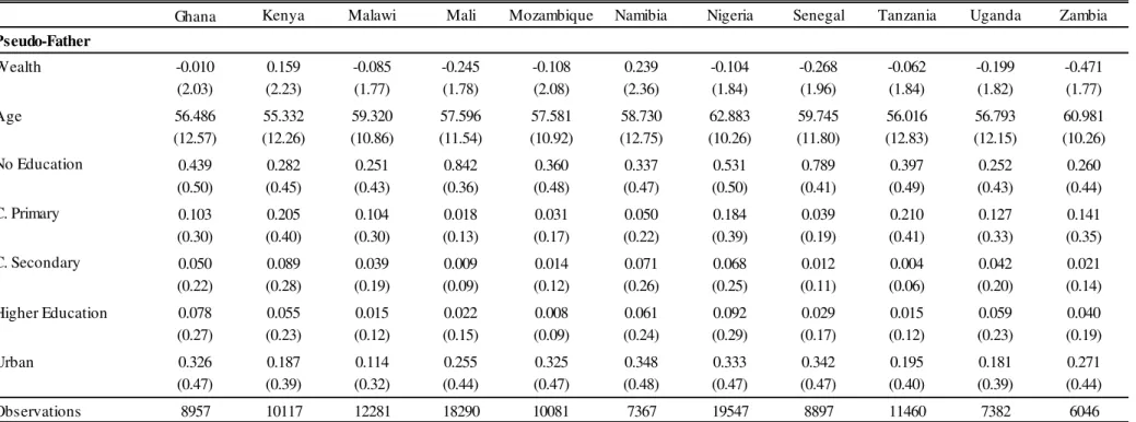
Ghana Kenya Malawi Mali Mozambique Namibia Nigeria Senegal Tanzania Uganda Zambia
Pseudo-Father
Wealth -0.010 0.159 -0.085 -0.245 -0.108 0.239 -0.104 -0.268 -0.062 -0.199 -0.471
(2.03) (2.23) (1.77) (1.78) (2.08) (2.36) (1.84) (1.96) (1.84) (1.82) (1.77)
Age 56.486 55.332 59.320 57.596 57.581 58.730 62.883 59.745 56.016 56.793 60.981
(12.57) (12.26) (10.86) (11.54) (10.92) (12.75) (10.26) (11.80) (12.83) (12.15) (10.26)
No Education 0.439 0.282 0.251 0.842 0.360 0.337 0.531 0.789 0.397 0.252 0.260
(0.50) (0.45) (0.43) (0.36) (0.48) (0.47) (0.50) (0.41) (0.49) (0.43) (0.44)
C. Primary 0.103 0.205 0.104 0.018 0.031 0.050 0.184 0.039 0.210 0.127 0.141
(0.30) (0.40) (0.30) (0.13) (0.17) (0.22) (0.39) (0.19) (0.41) (0.33) (0.35)
C. Secondary 0.050 0.089 0.039 0.009 0.014 0.071 0.068 0.012 0.004 0.042 0.021
(0.22) (0.28) (0.19) (0.09) (0.12) (0.26) (0.25) (0.11) (0.06) (0.20) (0.14)
Higher Education 0.078 0.055 0.015 0.022 0.008 0.061 0.092 0.029 0.015 0.059 0.040
(0.27) (0.23) (0.12) (0.15) (0.09) (0.24) (0.29) (0.17) (0.12) (0.23) (0.19)
Urban 0.326 0.187 0.114 0.255 0.325 0.348 0.333 0.342 0.195 0.181 0.271
(0.47) (0.39) (0.32) (0.44) (0.47) (0.48) (0.47) (0.47) (0.40) (0.39) (0.44)
Observations 8957 10117 12281 18290 10081 7367 19547 8897 11460 7382 6046
Note:Pseudo-Fathers' Wealth, wealth of an individual born before 1960, head of household. No Education, dummy variable, 1 if individual has no education and 0 otherwise. C. Primary, dummy variable, 1 if individual has completed primary school and 0 otherwise. C. Secondary, dummy variable, 1 if individual has completed secondary schooling and 0 otherwise. Higher Education, dummy variable, 1 if an individual studies after secondary school and 0 otherwise. Age, age of an individual measured in years. Urban, dummy variable, 1 if individual lives in an urban area and 0 if it lives in a rural area. First row means, Second row (in parenthesis) standard deviations.
- 28 - Table A.1: Descriptive Statistics - Demographic and Health Survey (continue)
Ghana Kenya Malawi Mali Mozambique Namibia Nigeria Senegal Tanzania Uganda Zambia
Father
P. Wealth -0.918 -0.270 -0,1145 -0.237 -0.290 0.310 -0.569 -0.627 -0.248 -0.539 -0.349
(1.02) (1.41) (1.05) (1.06) (1.19) (1.61) (0.99) (1.01) (1.02) (1.08) (1.25)
Age 72.703 68.846 67.193 69.204 65.149 64.089 70.537 72.419 68.120 64.419 67.613
(11.54) (11.04) (12.90) (9.98) (11.53) (13.58) (10.91) (11.59) (11.40) (13.32) (10.21)
No Education 0.812 0.654 0.303 0.936 0.486 0.429 0.753 0.946 0.608 0.547 0.360
(0.39) (0.48) (0.46) (0.24) (0.50) (0.50) (0.43) (0.23) (0.49) (0.50) (0.48)
C. Primary 0.029 0.115 0.084 0.000 0.000 0.000 0.124 0.011 0.136 0.105 0.040
(0.17) (0.32) (0.28) (0.00) (0.00) (0.00) (0.33) (0.10) (0.34) (0.31) (0.03)
C. Secondary 0.000 0.038 0.017 0.013 0.000 0.089 0.026 0.000 0.000 0.012 0.973
(0.00) (0.19) (0.13) (0.11) (0.00) (0.29) (0.16) (0.00) (0.00) (0.11) (0.16)
Higher Education 0.029 0.000 0.000 0.006 0.000 0.018 0.016 0.007 0.016 0.012 0.000
(0.17) (0.00) (0.00) (0.08) (0.00) (0.13) (0.12) (0.08) (0.13) (0.11) (0.00)
Urban 0.159 0.192 0.126 0.331 0.365 0.446 0.205 0.204 0.184 0.140 0.400
(0.37) (0.40) (0.33) (0.47) (0.48) (0.50) (0.40) (0.40) (0.39) (0.35) (0.49)
Observations 138 52 119 157 74 56 380 279 125 86 75
- 29 - Table A.1: Descriptive Statistics - Demographic and Health Survey (continue)
Ghana Kenya Malawi Mali Mozambique Namibia Nigeria Senegal Tanzania Uganda Zambia
Son
Wealth -1.038 0.099 -0.061 -0.055 -0.020 0.650 -0.444 -0.806 0.232 -0.513 0.436
(1.48) (2.28) (1.56) (1.99) (2.15) (2.29) (1.71) (1.65) (2.15) (1.06) (2.36)
Age 31.529 31.865 30.630 34.318 29.797 32.500 33.811 36.742 32.936 31.605 33.293
(6.83) (6.80) (6.93) (6.35) (7.10) (7.62) (7.96) (6.79) (6.92) (7.67) (8.01)
No Education 0.449 0.173 0.084 0.631 0.095 0.161 0.268 0.746 0.088 0.093 0.040
(0.50) (0.38) (0.28) (0.48) (0.29) (0.37) (0.44) (0.44) (0.28) (0.29) (0.20)
C. Primary 0.065 0.212 0.126 0.013 0.068 0.054 0.182 0.050 0.624 0.151 0.280
(0.25) (0.41) (0.33) (0.11) (0.25) (0.23) (0.39) (0.22) (0.49) (0.36) (0.45)
C. Secondary 0.065 0.192 0.134 0.013 0.027 0.179 0.224 0.004 0.000 0.023 0.120
(0.25) (0.40) (0.34) (0.11) (0.16) (0.39) (0.42) (0.06) (0.00) (0.15) (0.33)
Higher Education 0.014 0.077 0.000 0.032 0.014 0.018 0.134 0.018 0.016 0.058 0.067
(0.12) (0.27) (0.00) (0.18) (0.12) (0.13) (0.34) (0.13) (0.13) (0.24) (0.25)
Observations 138 52 119 157 74 56 380 279 125 86 75
- 30 -
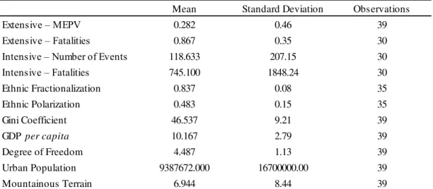
Mean Standard Deviation Observations
Extensive – MEPV 0.282 0.46 39
Extensive – Fatalities 0.867 0.35 30
Intensive – Number of Events 118.633 207.15 30
Intensive – Fatalities 745.100 1848.24 30
Ethnic Fractionalization 0.837 0.08 35
Ethnic Polarization 0.483 0.15 35
Gini Coefficient 46.537 9.21 39
GDPper capita 10.167 2.79 39
Degree of Freedom 4.487 1.13 39
Urban Population 9387672.000 16700000.00 39
Mountainous Terrain 6.944 8.44 39
Table A.2: Descriptive Statistics - Political Violence and other variables
- 31 -
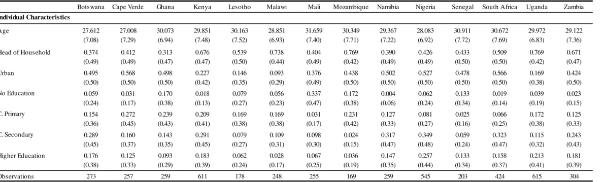
Botswana Cape Verde Ghana Kenya Lesotho Malawi Mali Mozambique Namibia Nigeria Senegal South Africa Uganda Zambia
Age 27.612 27.008 30.073 29.851 30.163 28.851 31.659 30.349 29.367 28.083 30.911 30.672 29.972 29.122
(7.08) (7.29) (6.94) (7.48) (7.52) (6.93) (7.40) (7.71) (7.22) (6.92) (7.72) (7.69) (6.83) (7.36)
Head of Household 0.374 0.412 0.313 0.676 0.539 0.738 0.404 0.769 0.390 0.426 0.433 0.509 0.769 0.671
(0.49) (0.49) (0.47) (0.47) (0.50) (0.44) (0.49) (0.42) (0.49) (0.49) (0.50) (0.50) (0.42) (0.47)
Urban 0.495 0.568 0.498 0.227 0.146 0.093 0.376 0.438 0.502 0.527 0.478 0.566 0.169 0.424
(0.50) (0.50) (0.50) (0.42) (0.35) (0.29) (0.49) (0.50) (0.50) (0.50) (0.50) (0.50) (0.38) (0.50)
No Education 0.059 0.031 0.170 0.018 0.079 0.056 0.337 0.172 0.004 0.062 0.133 0.019 0.039 0.023
(0.24) (0.17) (0.38) (0.13) (0.27) (0.23) (0.47) (0.38) (0.06) (0.24) (0.34) (0.14) (0.19) (0.15)
C. Primary 0.154 0.272 0.239 0.209 0.169 0.169 0.031 0.231 0.127 0.081 0.025 0.066 0.172 0.125
(0.36) (0.45) (0.43) (0.41) (0.38) (0.38) (0.17) (0.42) (0.33) (0.27) (0.16) (0.25) (0.38) (0.33)
C. Secondary 0.289 0.160 0.143 0.291 0.079 0.109 0.098 0.024 0.317 0.349 0.059 0.323 0.115 0.243
(0.45) (0.37) (0.35) (0.45) (0.27) (0.31) (0.30) (0.15) (0.47) (0.48) (0.24) (0.47) (0.32) (0.43)
Higher Education 0.176 0.125 0.093 0.183 0.062 0.028 0.067 0.036 0.147 0.257 0.133 0.158 0.213 0.181
(0.38) (0.33) (0.29) (0.39) (0.24) (0.17) (0.25) (0.19) (0.35) (0.44) (0.34) (0.37) (0.41) (0.39)
Observations 273 257 259 611 178 248 255 169 259 545 203 424 615 304
Table A.3: Descriptive Statistics - Afrobarometer
Individual Characteristics
- 32 -
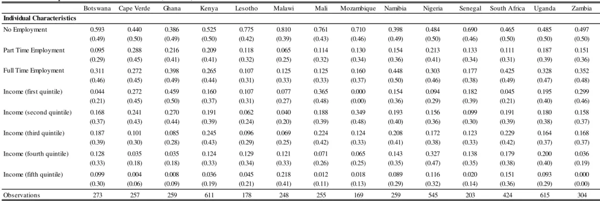
Botswana Cape Verde Ghana Kenya Lesotho Malawi Mali Mozambique Namibia Nigeria Senegal South Africa Uganda Zambia
No Employment 0.593 0.440 0.386 0.525 0.775 0.810 0.761 0.710 0.398 0.484 0.690 0.465 0.485 0.497
(0.49) (0.50) (0.49) (0.50) (0.42) (0.39) (0.43) (0.46) (0.49) (0.50) (0.46) (0.50) (0.50) (0.50)
Part Time Employment 0.095 0.288 0.216 0.209 0.118 0.065 0.114 0.130 0.154 0.213 0.133 0.111 0.187 0.151
(0.29) (0.45) (0.41) (0.41) (0.32) (0.25) (0.32) (0.34) (0.36) (0.41) (0.34) (0.31) (0.39) (0.36)
Full Time Employment 0.311 0.272 0.398 0.265 0.107 0.125 0.125 0.160 0.448 0.303 0.177 0.425 0.328 0.352
(0.46) (0.45) (0.49) (0.44) (0.31) (0.33) (0.33) (0.37) (0.50) (0.46) (0.38) (0.49) (0.47) (0.48)
Income (first quintile) 0.044 0.272 0.459 0.160 0.107 0.077 0.365 0.000 0.154 0.094 0.182 0.045 0.195 0.299
(0.21) (0.45) (0.50) (0.37) (0.31) (0.27) (0.48) (0.00) (0.36) (0.29) (0.39) (0.21) (0.40) (0.46)
Income (second quintile) 0.168 0.241 0.270 0.191 0.062 0.040 0.188 0.349 0.193 0.156 0.099 0.191 0.180 0.158
(0.37) (0.43) (0.44) (0.39) (0.24) (0.20) (0.39) (0.48) (0.40) (0.36) (0.30) (0.39) (0.38) (0.37)
Income (third quintile) 0.187 0.101 0.085 0.245 0.096 0.069 0.224 0.124 0.208 0.172 0.123 0.229 0.164 0.168
(0.39) (0.30) (0.28) (0.43) (0.29) (0.25) (0.42) (0.33) (0.41) (0.38) (0.33) (0.42) (0.37) (0.37)
Income (fourth quintile) 0.128 0.035 0.035 0.124 0.129 0.121 0.071 0.065 0.143 0.327 0.138 0.179 0.200 0.036
(0.33) (0.18) (0.18) (0.33) (0.34) (0.33) (0.26) (0.25) (0.35) (0.47) (0.35) (0.38) (0.40) (0.19)
Income (fifth quintile) 0.099 0.004 0.008 0.036 0.045 0.218 0.012 0.018 0.089 0.116 0.020 0.151 0.093 0.000
(0.30) (0.06) (0.09) (0.19) (0.21) (0.41) (0.11) (0.13) (0.29) (0.32) (0.14) (0.36) (0.29) (0.00)
Observations 273 257 259 611 178 248 255 169 259 545 203 424 615 304
Table A.3: Descriptive Statistics - Afrobarometer (continue)
Individual Characteristics
Note:No Employment, dummy variable, 1 if individual is not employed and 0 otherwise. Part Time Employment, dummy variable, 1 if individual is employed part time and 0 otherwise. Full Time Employment, dummy
- 33 -
Botswana Cape Verde Ghana Kenya Lesotho Malawi Mali Mozambique Namibia Nigeria Senegal South Africa Uganda Zambia
School 0.626 0.665 0.946 0.766 0.652 0.851 0.616 0.899 0.625 0.895 0.926 0.788 0.954 0.822
(0.48) (0.47) (0.23) (0.42) (0.48) (0.36) (0.49) (0.30) (0.48) (0.31) (0.26) (0.41) (0.21) (0.38)
Police 0.527 0.187 0.301 0.182 0.146 0.089 0.071 0.349 0.432 0.442 0.300 0.455 0.260 0.293
(0.50) (0.39) (0.46) (0.39) (0.35) (0.28) (0.26) (0.48) (0.50) (0.50) (0.46) (0.50) (0.44) (0.46)
Health Clinic 0.344 0.237 0.548 0.340 0.219 0.294 0.376 0.473 0.332 0.719 0.581 0.566 0.654 0.569
(0.48) (0.43) (0.50) (0.47) (0.41) (0.46) (0.49) (0.50) (0.47) (0.45) (0.49) (0.50) (0.48) (0.50)
Electricity Grid 0.857 0.837 0.625 0.409 0.270 0.218 0.310 0.391 0.421 0.694 0.576 0.830 0.231 0.513
(0.35) (0.37) (0.48) (0.49) (0.45) (0.41) (0.46) (0.49) (0.49) (0.46) (0.50) (0.38) (0.42) (0.50)
Piped Water 0.850 0.607 0.591 0.339 0.281 0.194 0.357 0.426 0.502 0.490 0.571 0.821 0.158 0.401
(0.36) (0.49) (0.49) (0.47) (0.45) (0.40) (0.48) (0.50) (0.50) (0.50) (0.50) (0.38) (0.36) (0.49)
Sewage 0.392 0.366 0.328 0.146 0.180 0.036 0.192 0.243 0.421 0.347 0.315 0.677 0.091 0.257
(0.49) (0.48) (0.47) (0.35) (0.39) (0.19) (0.39) (0.43) (0.49) (0.48) (0.47) (0.47) (0.29) (0.44)
Observations 273 257 259 611 178 248 255 169 259 545 203 424 615 304
Location Characteristics
Table A.3: Descriptive Statistics - Afrobarometer (continue)
- 34 - Table A.4: IV First-Stage Regression
(1) (2) (3)
Availability of goods 0.186*** 0.214*** 0.184***
(0.03) (0.04) (0.03)
Individual Controls no no yes
Location Controls no no yes
Country Fixed Effects no yes yes
Observations 4832 4832 4832