Todos os direitos reservados.
É proibida a reprodução parcial ou integral do conteúdo
deste documento por qualquer meio de distribuição, digital ou
impresso, sem a expressa autorização do
REAP ou de seu autor.
Spillovers from Conditional Cash
Transfer Programs:
Bolsa Família
and Crime in Urban Brazil
Laura Chioda
João M. P. De Mello
Rodrigo R. Soares
SPILLOVERS FROM CONDITIONAL CASH TRANSFER PROGRAMS:
BOLSA FAMÍLIA
AND CRIME IN URBAN BRAZIL
Laura Chioda
João M. P. De Mello
Rodrigo R. Soares
Laura Chioda World Bank
Washington, D.C - United States
João Manoel de Pinho Mello
Pontifícia Universidade Católica do Rio de Janeiro (PUC-Rio) Departamento de Economia
Rua Marquês de São Vicente, nº 225 Gávea
22451-900 - Rio de Janeiro, RJ - Brazil [email protected]
Rodrigo R. Soares
Pontifícia Universidade Católica do Rio de Janeiro (PUC-Rio) Departamento de Economia
Rua Marquês de São Vicente, nº 225 Gávea
Spillovers from Conditional Cash Transfer Programs:
Bolsa Família
and Crime in Urban Brazil
Laura Chioda
João M. P. De Mello†
Rodrigo R. Soares‡
February 2012
Abstract
This paper investigates the impact of Conditional Cash Transfer (CCT) programs on crime. Making use of a unique dataset combining detailed school characteristics with time and geo-referenced crime information from the city of São Paulo, Brazil, we estimate the contemporaneous effect of the Bolsa Família program on crime. We address the endogeneity of CCT coverage by exploiting the 2008 expansion of the program to adolescents aged 16 and 17. We construct an instrument that combines the timing of expansion and the initial demographic composition of schools to identify plausibly exogenous variations in the number of children covered byBolsa Família. We find a robust and significant negative impact ofBolsa Famíliacoverage on crime. The evidence suggests that the main effect works through increased household income or changed peer group, rather than from incapacitation from time spent in school.
Keywords:Conditional Cash Transfer,Bolsa Família, Crime, Education, Schooling, Brazil JEL codes:I28, I38, K42
The authors wish to thank Tulio Kahn and Alexandre Schneider for help with the data, and Joana Simões de Melo Costa and Priscilla Burity for outstanding research assistance. This paper benefited from comments from Tito Cordella, Anna Fruttero, and seminar participants at the World Bank’s Workshop “Building the Evidence Base for Crime and Violence Prevention in Brazil” (Brasília, 2010), the 32nd Meeting of the Brazilian Econometrics Society, and the 16th LACEA Annual Meeting (Santiago, 2011). Contact information:lchiodaatworldbank.org,jmpmatecon.puc-rio.br, andsoaresatecon.puc-rio.br.
World Bank †
1. Introduction
Conditional Cash Transfer (CCT) programs, in which families receive government payments upon
fulfillment of schooling and other requirements, are today among the most popular and celebrated social
support programs in the world. Various versions of CCTs have been adopted in countries as diverse as
Argentina, Bangladesh, Colombia, Indonesia, Jamaica, Kenya, Mexico, Turkey, and the US, among innumerous
others. There is substantial evidence from some of these settings on the positive effects of CCTs on enrollment
rates, preventive health care, and nutrition (for reviews of the literature, see Rawlings and Rubio, 2005, and
Fizbein and Schady, 2009). Brazil, in particular, has one of the first and the largest CCT program in the world,
currently namedBolsa Família. It covers over 11 million families and costs close to 0.4% of the country’s GDP.
Evidence suggests that Bolsa Família has had substantial impact on enrollment rates, school progression,
extreme poverty, and inequality, though there are questions related to its social rate of return and
effectiveness in urban settings (Soares and Sátyro, 2009, and Glewwe and Kassouf, 2012).
This paper uses school and crime data from the city of São Paulo, Brazil, to present one of the first
pieces of evidence on the effect ofBolsa Família– or, for that matter, of any CCT program – on crime.1Making
use of a unique dataset combining detailed school characteristics with time and geo-referenced crime
information, we estimate the contemporaneous impact of the number of children covered by Bolsa Família
within a school on crime in the school neighborhood. The number of children covered by CCT in an area at a
moment in time is determined by the incidence of poverty and unemployment and by other socioeconomic
characteristics, all likely to be correlated with crime. This precludes the interpretation of the correlation
between Bolsa Família coverage and crime as causal. We overcome this problem by exploiting the 2008
expansion of the program to adolescents aged 16 and 17, from an initial setting where maximum age of
coverage was 15. We construct an instrument that combines the timing of expansion and the initial
demographic composition of schools to identify plausibly exogenous variations in the number of children
covered by the CCT. This instrument allows us to estimate the causal impact of Bolsa Família on crime. We
find a robust and significant negative impact of Bolsa Famíliatransfers on crime. Our estimate suggests that
the expansion ofBolsa Famíliabetween 2006 and 2009, corresponding to roughly 59 more students covered
per school, caused a 21% reduction in crime in school neighborhoods (94 fewer crimes per school per year).
1
While writing the final version of this paper, we became aware of the work of Loureiro (2012). The author analyzes the effect of
The potential relevance of CCTs as crime reducing instruments should indeed be expected, given that
youth account for a disproportionately high fraction of crimes, and that there is an intimate relationship
between education, socioeconomic conditions, and crime. In the US, for example, Levitt and Lochner (2001)
document that 20% of the arrests for violent crimes involve individuals between ages 15 and 19. In our data
for São Paulo, among crimes for which the age of the suspected offender is known, between 20% and 25% of
robberies, thefts, and motor vehicle crimes are supposedly committed by individuals below age 18.
On education and crime, there are various potential channels in a two-way relationship. There is
evidence on the effect of violence and crime on schooling and learning (see, for example, Grogger, 1997, Aizer,
2009, Rodríguez and Sanchez, 2009, Chambargwala and Morán, 2010, and Monteiro and Rocha, 2011) and
also on the effect of schooling on involvement with crime and violence (see review by Lochner, 2010).
Schooling may have long-term effects on criminal behavior through wages and preferences (discount rates
and risk aversion), and, therefore, through the relative attractiveness of criminal activities and the cost of
expected punishment (Becker and Mulligan, 1997, Lochner and Moretti, 2004, Lochner, 2010, Machin et al,
2010, and Deming, 2011). More importantly for this paper, schooling also has short-term impacts through an
incapacitation effect, since time spent in school reduces the opportunity for certain types of crimes and risky
behavior, though possibly also increasing the interaction among youth and the likelihood of violence.
Anderson (2011), for example, documents declines in juvenile crime rates at the time of increase in minimum
dropout ages across US states, while Berthelon and Kruger (2011) report reductions in crime and teenage
pregnancy following a school reform in Chile that increased weekly school hours from 32 to 39. Jacob and
Lefgren (2003) and Luallen (2006), the former exploiting variations in teacher in-service days and the latter
teacher strikes, document that property crimes decline but violent crimes rise when youth are in school (see
also Snyder and Sickmund, 1999, and Gottfredson and Soulé, 2005).
But one of CCTs’ main features is that it also implies monthly money transfers to families, and these
may have direct impacts on criminal behavior. The ability to buy certain goods with transfers from the
government may reduce the incentive or “need” to engage in economically motivated crimes. Additional
income from welfare transfers may also alter households’ routines in a manner that exposes them to less risk
of victimization and/or opportunities for delinquency, such as by affording parents more time for supervision
(Heller et al, 2010). Indeed, there is evidence that welfare transfers affect crime rates. De Franzo (1996, 1997),
Zhang (1997), Hannon and De Franzo (1998), and Foley (2008) study the effect of the amount and timing of
welfare payments, finding impacts on total number of crimes (negative) and also on the distribution of crimes
the equivalent of 50% of household income to beneficiaries, reporting a decline of roughly 20% in both violent
and overall arrests, which implies an income elasticity of -0.4.
A final channel through which CCTs may affect crime is social interaction. If the network or reference
group of youth is affected by school enrollment and attendance, then staying in school may have positive peer
effects (Glaeser et al, 1996, and Lochner, 2010), despite the higher probability of attrition between youths.
This would be true as long as the school network were on average better than the peer group that youth
would have in case they dropped out (or did not attend school).
The main challenge faced by this paper is to isolate the channel through which Bolsa Famíliaaffects
crime. Though we present robust evidence on the effect ofBolsa Famíliatransfers on crime, we are not able
to directly address the issue of channel. Nevertheless, by looking at the heterogeneity of effects across days
and types of crimes, we do provide some suggestive evidence on the channels that are likely to be at work in
our setting. We find that the estimated effects of CCT on crime are virtually identical across school and
non-school days, suggesting that the incapacitation mechanism extensively discussed in the US literature is not the
driving force behind our results. We also find the effects to be quantitatively more important for robberies,
though there is also some evidence of reductions in drug-related crimes and crimes against minors. So the
results indicate that the income component of Bolsa Famíliais likely to be an important determinant of the
reductions in crime, though social interactions through changed peer groups cannot be ruled out.
Our paper relates to three strands of literature. First, the paper adds to the numerous studies analyzing
the impact of CCT programs by showing that spillovers onto other social phenomena, not directly targeted in
the initial design of this type of program, may be significant and relevant from a policy perspective (see review
in Fizbein and Schady, 2009). Second, it relates to the literature on educational policies and crime, and
presents a context in which there is a reduction crime, but where incapacitation and future returns to
schooling do not seem to be the main thrust. And third, the paper also speaks to the discussion on the
socioeconomic determinants of crime. Various authors have documented a robust correlation between
inequality and crime (see, for example, Fajnzylber et al, 2002, Bourguignon et al, 2003, Soares, 2004, or the
discussion in Soares and Naritomi, 2010). To the extent that Bolsa Família has had a substantial impact on
inequality in Brazil (Soares and Sátyro, 2009), and that the income effect is likely to be an important force
behind our results, the evidence presented here may be seen as an additional piece of information on the
relationship between socioeconomic conditions and crime (in line with the evidence from welfare payments
The remainder of the paper is organized as follows. Section 2 provides an institutional background, by
briefly describing the Bolsa Família CCT program and Brazilian educational and law enforcement systems.
Section 3 presents and discusses the data, while section 4 describes our methodology and identification
strategy. Finally, section 5 presents the results and is followed by concluding remarks in section 6.
2. Institutional Background
2.1 The Bols a F amí li a Conditional Cash Transfer Program
Bolsa Família(or “Family Allowance”) is Brazil’s federal CCT program, created in 2003. Its creation was,
in fact, the consolidation of various social support programs coupled with a redesign of Brazil’s first federal
CCT program,Bolsa Escola, which had been in operation since 2001. Bolsa Escola, in turn, was inspired by a
series of pilot projects in various Brazilian cities, dating back to 1995 in the capital Brasília, and in Campinas
and Ribeirão Preto, both in the state of São Paulo. Soares and Sátyro (2009) provide a history ofBolsa Família
and a detailed discussion of its institutional design, as well as references to various impact evaluation studies.
Bolsa Família currently provides different benefits for families at different income levels and has
various conditionalities. The Basic Benefit is a payment of R$60.00 for families with monthly per capita (p.c.)
income below R$70.00. In addition, there is the Variable Benefit, according to which families with monthly p.c.
income below R$140.00 receive R$22.00 per child under age 15 (up to the maximum of 3 payments). Finally,
starting in 2008, benefits were extended to adolescents, through the creation of the Variable Youth Benefit.
The Variable Youth Benefit paid R$33.00 per family member aged between 16 and 17 (up to a maximum of 2
payments), for families with monthly p.c. income below R$140.00.2
The maximum benefit value in Bolsa Família is R$200.00 per family, which applies to families with
monthly p.c. income below R$70.00, 3 children under age 15, and 2 adolescents aged between 16 and 17.
There are also schooling and health conditionalities attached to the payments, though recently it has been
claimed that they are not seriously enforced. In terms of schooling, program participation requires school
enrollment and 85% attendance for children between 6 and 15, and 75% attendance for adolescents between
16 and 17. Regarding health, conditionalities include fulfillment of a vaccination and growth and development
calendar for children under 7, prenatal care for pregnant women, and health monitoring for lactating women.
It is important to mention that, during the period of our analysis, there was a second CCT program in
operation in the city of São Paulo: the municipal programRenda Mínima(or “Minimum Income”). São Paulo’s
Renda Mínimais a minimum family income program created in 2006. In order to be eligible for the program,
2
families must have lived in the city of São Paulo for at least 2 years, have monthly p.c. income below R$175.00,
and have at least one child under age 16. The conditionalities are school enrollment and minimum attendance
of 85% for children between ages 6 and 15, and fulfillment of a vaccination calendar for children under 7.
Renda Mínima’s benefits can complement those of Bolsa Família. The maximum benefits allowed byRenda
Mínima are (total value = Bolsa Família + Renda Mínima): R$140.00 for families with 1 child, R$170.00 for
families with 2 children, and R$200.00 for families with 3 or more children.
Renda Mínimais sometimes used as a complement toBolsa Família, while sometimes families receive
only one of the two benefits. Our CCT data, to be discussed in further detail below, is on the number of
students per school receivingBolsa FamíliaandRenda Mínima(with no information on value). The correlation
of the number of Bolsa Família and Renda Mínima recipients across schools is above 0.75, making it very
difficult to separate the independent effect of each program. In addition, we have an institutional change in
Bolsa Família that allows us to identify its causal impact, so we concentrate our analysis on the impact of the
federal CCT program (also, the number of students covered byBolsa Famíliais 18% higher than that ofRenda
Mínima). We do however check whether results change if we incorporateRenda Mínimain the analysis and,
more importantly, we useRenda Mínimaas a way to validate our instrument.
Regarding the operational aspects of the program, Bolsa Família is federally funded and jointly
managed by the federal and municipal governments. Budgets for the program for each municipality are
determined by the federal government, based on estimates of the number of poor families. Applications of
families, eligibility verification, and final decisions on enrollment are managed by the municipality, conditional
on the budget determined by the federal government (Glewwe and Kassouf, 2012). Schools play no direct role
in operating or funding the program, apart from recording children’s attendance. Payments are done by the
Ministry of Social Development directly to individual family accounts, which can be accessed using bank cards
distributed to families.
Thus, in our particular context, it is very unlikely that CCT allocation takes into account differences in
violence within the city of São Paulo. However, the program targets poor families, and areas with different
concentration – or dynamics – of poverty are likely to have different levels – or dynamics – of crime, be it due
to socioeconomic conditions, to other policies, or to different intensity and style of policing.
2.2 Law Enforcement
Law enforcement in Brazil is primarily the responsibility of state governments. Executive and
administrative authority rests with the state secretariats of public security (Secretarias Estaduais de Segurança
secretariats. Some strategic decisions are determined by law. For example, by constitutional mandate, the
number of policemen in the state of São Paulo has to be roughly constant in per capita terms across cities. The
execution of enforcement is shared between two corporations that respond to the secretariats: the military
police, responsible for ostensive patrolling and repression, and the civil police, which is judiciary and
investigative. The commanders of the two police forces are appointed by the governor. There are also
municipal police forces (Guardas Civis Municipais), which are not mandatory by federal law but a choice of the
municipality. These can be used to reinforce ostensive patrolling, traffic and crowd control, but have less
authority and a reduced scope in comparison to the state polices. The city of São Paulo has its municipal police
force. Crime recording and monitoring of public security conditions are, nevertheless, responsibility of the
state polices.
2.3 Education
Primary and secondary schooling in Brazil is mainly responsibility of cities and states. In general, cities
focus on elementary and middle schools (pre-school to 8th grade), and states focus on middle and high
schools. In the city of São Paulo, 98% of municipal schools offer middle school grades and none offers high
school, while, among state schools, 93% offer middle school grades and 99% offer high school.
Pupil allocation to schools is based on residence location. There are no official school districts, but the
city and state secretariats form a committee, which enroll the pupil at the closest available school. Once the
child enters a school, she stays there unless the family moves from the original neighborhood. Parents cannot
choose schools, except for a couple of high-performance flagship schools – which have enrollment rationed
through entrance exams – and for decisions on neighborhood of residence. There is no evidence that public
schooling is an important dimension in neighborhood choice in Brazil.
Given the system of assignment of pupils to schools, it is unlikely that students with particular
characteristics (more or less violent, for example) are deliberately sent to schools with more Bolsa Família
coverage. However, again, students from poorer families will be clustered in schools in poorer neighborhoods,
which are likely to have higher coverage of Bolsa Família and higher crime rates. Similarly, changes in local
economic conditions and other policies may simultaneously affect eligibility of families to the CCT program
and the incidence of crime in a certain area. To give a concrete example, consider the minimum wage increase
from R$300 to R$465 between 2006 and 2009, corresponding to a 55% gain in nominal terms and a 30% gain
in real terms. To the extent that minimum wages impact mostly low-income families, this change should affect
the correlation between CCT coverage and crime. This is the type of concern we have in mind when
3. Data
3.1 Crime Data
Our crime data are from the INFOCRIM database, a COMPSTAT-like crime tracking system from the
Secretaria de Segurança Pública do Estado de São Paulo, the state law enforcement agency. We have time and
geo-referenced data for all reported crimes in the city of São Paulo, from 2006 through 2009. INFOCRIM
includes all information available from the police reports. It includes location of occurrence (translated into
latitude and longitude), type of crime, estimated time of occurrence, and, sometimes, characteristics of the
suspected offender, such as age and gender. Unfortunately, age of the suspected offender is available only for
a very small fraction of the sample. Therefore, due to concerns about sample selection, we do not use this
specific information. We concentrate our analysis on thefts, robberies, acts of vandalism, violent crimes,
drug-related offenses, and crimes against minors.3 Records related to these offenses encompass a total of
1,473,939 crimes over the 4 years in our sample.
3.2 School Data
Our school and student data cover the period between 2006 and 2009 and come from two sources.
From the Secretaria de Educação da Cidade de São Paulo, we have data on state and municipal schools
identifying the type of school, school location (translated into longitude and latitude), and number of students
covered by conditional cash transfer programs (separate information on number of students receiving Bolsa
Família and Renda Mínima). From the Brazilian School Census, we gather additional information on number
and demographic characteristics of teachers and students, and school infrastructure. The characteristics are:
education of teachers; gender, race, and current grade of students; and number of classrooms, availability of
treated water, sanitation, and TV, and number of computers.
3.3. Unit of Analysis
Given the data, nature of the phenomenon, and policy we are studying, geographic areas associated
with particular schools should be the natural unit of analysis. Unfortunately, as mentioned before, São Paulo
does not have a strict geographic definition of school districts. Still, students in the city are allocated to slots
available in the closest school, so there is a high correlation between school location and neighborhood of
3
residence. Therefore, we create artificial school districts by assigning to a given school the area that is closer
to it than to any other school.
This is a key step that allows us to link crimes happening in a given location to a particular school.
Obviously, children do not circulate only in these areas and do not necessarily live there, but they are likely to
live close to the school and spend part of their day there. If there is a high probability that children are around
the school area for a significant amount of time, this approach should be adequate. US evidence supports this
strategy, since it reveals a concentration of crimes committed by youth in periods immediately after school
hours, when children/adolescents are still likely to be near the school (Snyder and Sickmund, 1999, Jacob and
Lefgren, 2003, and Gottfredson and Soulé, 2005). The system of allocation of students to schools in São Paulo
also supports our approach, as children are expected to study in the closest school available. Hence, our
measure of crime per school is the number of crimes that were committed closer to a given school than to any
other school (these crimes are “assigned” to that particular school).4
The construction of our dependent variable depends, therefore, on the schools included in the sample.
Generally, the number of crimes assigned to a given school can vary with the full set of schools considered.
Given the typical age of students, we focus on middle and high schools (from 5thto 11thgrade) and start by
generating the number of crimes per school considering three different samples: only high schools, only
middle schools, and middle schools and high schools together.5This allows us to check the robustness of the
results to different formulations and also to assess how the response of crime varies with the age of children.
Based on the age composition of students, it is likely that high schools – with older adolescents – would be the
more adequate unit for our analysis.
3.4 Descriptive Statistics
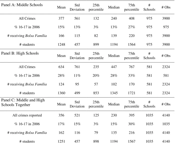
Table 1 provides descriptive statistics for the three samples we generate: one composed only of middle
schools, another composed only of high schools, and a third one composed of middle schools and high schools
together. The unit of observation is the school, and all crime statistics refer to the definition of school districts
discussed in the previous section.
High schools are less numerous than middle schools. Thus, by construction of our metric of crime
around schools, there is more crime around high schools than middle schools, since the former covers a larger
area than the latter. Otherwise, crime follows similar patterns around high and middle schools. Regarding
4
For each crime, we calculate the distance from the location of occurrence to every school in the sample. We subsequently assign that crime to the closest school.
5
specific types of crimes (not shown in the table), robbery is the most common, followed by violent crimes. The
incidence of theft is lower than that of violent crimes, suggesting a considerable degree of underreporting for
lesser crimes. Categories such as vandalism, drug-related and crimes against minors have substantially fewer
occurrences, indicating that it may be difficult to estimate the impact ofBolsa Famíliafor these categories.
Table 1 also presents descriptive statistics for the fraction of students aged between 16 and 17 in 2006,
which plays an important role in the construction of our instrument and the identification of the causal effect
of Bolsa Família(see next section). In high schools, 28% of pupils were 16 and 17 years old in 2007, with a
standard deviation of 11%. This is important for our purposes because our main strategy relies on the
presence and variation of 16 and 17 olds across schools. In middle schools, the fraction of 16 and 17
year-olds is smaller, as expected.
High schools have on average 1,360 students, whereas middle schools have 1,248 students. Finally,
Bolsa Família covers 9% of high school students and 13% of middle school students. The higher coverage in
middle schools is expected because, until 2008, eligibility toBolsa Famíliawas restricted to children below age
15. Also notice that there is substantial variation in the number of children covered by the CCT across schools,
reflecting both different number of students and different socioeconomic conditions across areas.
4. Empirical Strategy
The main challenge in the identification of the causal effect of CCTs on crime comes from the fact that
targeting implies that CCT coverage is correlated with socioeconomic conditions, which, in turn, can be
correlated with crime. This potential problem is present in both the cross section – as when poorer areas have
higher CCT coverage and higher crime – and the time series – as when areas experiencing economic
improvements see reductions in CCT coverage and reductions in crime rates. So, for example, fixed-effects,
despite being important for controlling for unobserved characteristics, would not be enough to overcome the
endogeneity problem. In short, the fraction of children covered by the program each year is likely to be a
direct function of socioeconomic conditions in the area at that point in time, which may in turn have an
independent impact on crime rates. From this perspective, we could find a positive correlation between CCTs
and crime simply because increased coverage is associated with deteriorating socioeconomic conditions.
In addition to controlling for school fixed-effects and several variables related to infrastructure and
teachers and students characteristics, we adopt an instrumental variables approach to try to overcome this
problem. As mentioned before, in 2008Bolsa Família extended its benefits to adolescents between ages 16
would receive R$33.00 per family member between ages 16 and 17, up to a maximum of 2. Relying on the
different demographic composition of schools, we can construct an instrument for CCT coverage that exploits
the interaction of number of students between 16 and 17 in the first year in the sample (2006) with the timing
of program expansion. If there is an impact of conditional cash transfers on crime, then whenBolsa Famíliais
expanded one should expect a larger reduction in crime around schools that had a higher fraction of students
between 16 and 17 before program expansion.
Our benchmark specification is the following:
݈݊(ܿݎ݅݉݁௧) =ߙ+ߚ(ܥܥܶ௧) +ߛ’ܺ௧ +ߠ +ߜ௧ +ߝ௧, (1) where crimeitdenotes the number of crimes in schooli and yeart;CCTit is the number of students receiving
CCT;Xitis a set of school variables related to infrastructure, and teachers and students characteristics; andθi
and δtare, respectively, school and year fixed-effects. In all specifications, standard errors are clustered at the
school level, so that the error term is allowed to have an arbitrary correlation within schools over time. Our
instrument forCCTitis the interaction of number of students between ages 16 and 17 in 2006 with a dummy
variable equal to one in 2008 and 2009, years in which program coverage was expanded to those ages.
As we do not have a measure of local population, which would be the natural way to normalize the
number of crimes in a given area, we use the natural logarithm of number of crimes as the dependent
variable. We control for the number of children in the school in the right hand side, since they are potential
offenders and victims. Furthermore, given that children from different schools interact and migrate across
boundaries of our definition of school districts, in some specifications we also control for the number of
children in neighboring schools. To construct this variable, we count the number of students enrolled in
schools within two kilometers of a given school.
Our full set of controls includes the following information from the Brazilian School Census: number of
students enrolled, average years of schooling of teachers, student-teacher ratio, number of students per class,
availability of sewage, availability of treated water, availability of TVs for students, availability of computers
for students, fraction of non-white students, fraction of female students, fraction of delayed students, and, in
some specifications, number of students enrolled in schools within 2 kilometers. These are intended to
capture, above all, socioeconomic conditions of the area where the school is located (or, similarly, of the
students’ families) and impacts of other competing policies that may have similar effects to those expected
from CCTs.
One last issue in our estimation is the fact that the dependent variable is the number of crimes in
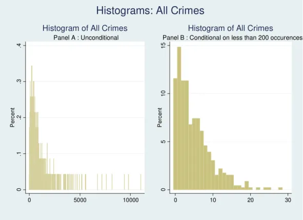
of the estimating equation, given the possibility of an excessive number of zeros and over-dispersion. In our
setting, excessive zeros do not seem to be a serious issue, but over-dispersion may be a problem (see Figure
A.1 in the Appendix). For this reason, in addition to linear regressions with the dependent variable in natural
logarithms (substituting undefined values by zero), we also estimate Poisson and negative binomial models. In
all three cases, coefficients can be interpreted as semi-elasticities.
Finally, in trying to understand the channels through which Bolsa Família affects crime, we also
estimate our benchmark specification for different types of crimes and for crimes committed in different days
of the week and at different hours.
5. Results
5.1 Benchmark Specification
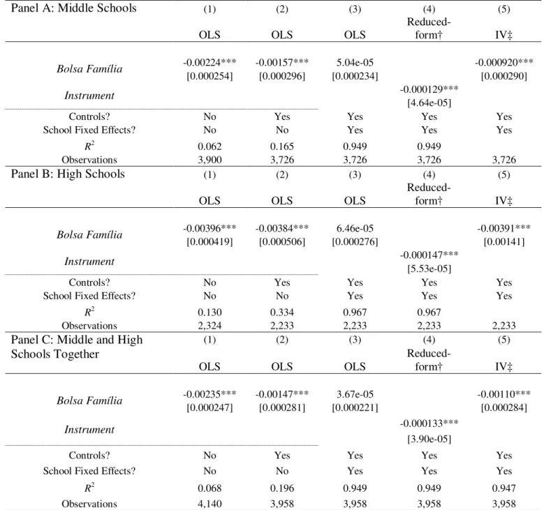
Panels A, B, and C in Table 2 present the results of our benchmark specification for the three
alternative samples: only middle schools, only high schools, and middle and high schools together. In order to
clarify the type of variation contained in the data and the role played by our instrument, each panel consists of
five columns: the first one displays the result of a simple regression of log of crimes on number of students
receiving Bolsa Famíla and time dummies, with no additional controls; the second column adds our set of
controls to this specification (students, teachers, and school characteristics); the third column adds school
fixed effects; the fourth columns presents a reduced form regression of log of crimes on our instrument and
the full set of controls (the instrument is the interaction of number of students between ages 16 and 17 in
2006 with a dummy equal to 1 in 2008 and 2009); and the last column presents our IV estimates, where
number of students receivingBolsa Famíliais treated as endogenous.
Qualitative results are identical across the three samples, so we concentrate the discussion on our
preferred sample, high schools, and leave quantitative considerations for later. Looking at column 1 in Panel B,
one can see a negative correlation between number of students receiving Bolsa Família and crime in the
school neighborhood. This correlation is not associated with observable characteristics of schools, teachers,
and students, since the coefficient remains virtually unchanged when we add the controls in column 2. But in
column 3, when we add school fixed effects, the negative correlation between CCT coverage and crime
disappears and the estimated coefficient becomes very small in magnitude and non-significant. These first
three columns suggests that there is some cross-sectional variation inBolsa Famíliacoverage that seems to be
negatively associated with crime, but that the within school variation in coverage bears no noticeable
in coverage across school, but coverage within a school over time responded to neighborhood conditions. The
latter would be expected if, for example, any improvement in local economic conditions were associated with
reducedBolsa Famíliaeligibility and reduced crime. The real gain in minimum wages mentioned before could
be one force generating this type of correlation, but any other factor determining local development would
also work in this direction.
The within school variation in CCT coverage seems to isolate the most endogenous dimension of
variation in our independent variable. Therefore, if we want to use school fixed effects to control for
unobserved neighborhood characteristics, we need to use our instrument forBolsa Famíliacoverage. Column
4 presents a reduced form regression of crime on our instrument, showing that the instrument is negatively
correlated with crime rates. In short, schools with a higher number of students between ages 16 and 17 in
2006 experienced larger declines in crime in 2008 and 2009, when the CCT coverage was expanded to these
age groups. In column 5, we use the instrument to isolate the supposedly exogenous dimension of variation in
Bolsa Família coverage. The coefficient is negative and statistically significant and, surprisingly, almost
identical to the coefficients presented in columns 1 and 2, where we did not use school fixed effects. So, for
the case of high schools, the simple conditional correlation between CCT coverage and crime seems to give a
very accurate estimate of the causal effect. The key identifying assumption here is that the age composition of
schools in 2006 was indeed associated with changes in coverage after 2008 and that, additionally, there was
no other connection between age composition and variations in crime apart from that working through CCT
coverage.6We present some evidence to support these two assumptions in the following tables.
The results across the three samples in Table 2 are qualitatively very similar, but have some noticeable
quantitative differences. First and most importantly, the estimated effects of Bolsa Família on crime are
stronger for high schools than for the other two samples. Since high schools have the older children and
adolescents, which indeed should be expected to be more actively involved in crime, this should be expected.
Overall, the estimated coefficients for high schools are at least 100% larger than the analogous ones for the
other two samples. Furthermore, the coefficient is much more stable across columns 1, 2 and 5 in the high
school sample. This suggests that, looking at column 1, the endogenous dimension of variation inBolsa Família
is a more serious issue for middle schools than for high schools. For all these reasons, and also because high
schools constituted our preferred sample since the beginning, we concentrate the results presented in the
remainder of the paper on the high school sample and on the specification from column 5.
6
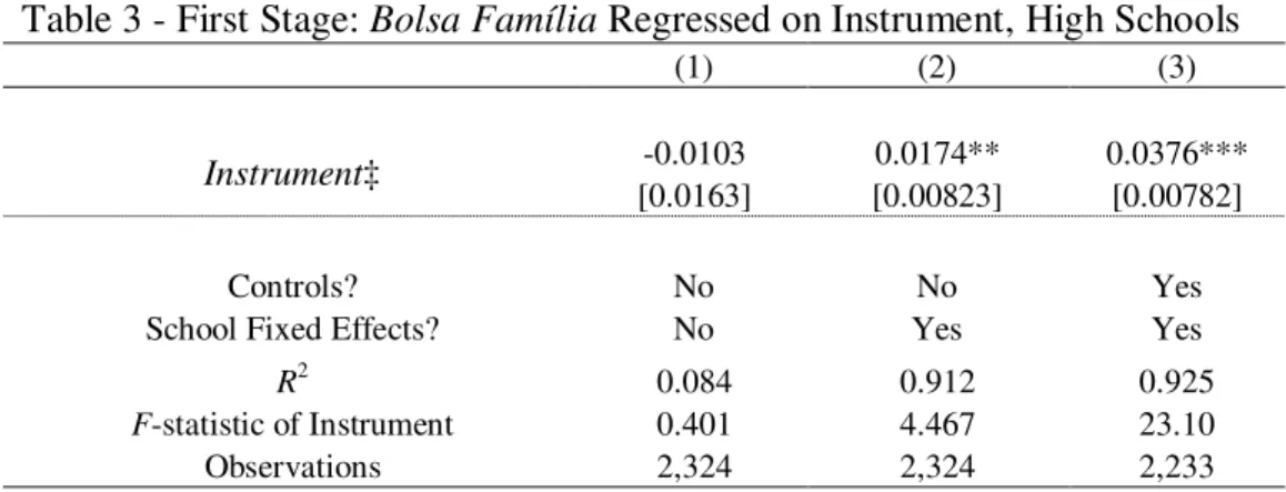
Table 3 presents the first stage of our instrumental variable strategy. In order to clarify the type of
variation identified by the instrument, we present three specifications: the first one is a simple regression of
Bolsa Família coverage on the instrument and time dummies; the second one includes school fixed effects;
and the last one, which is the actual first stage related to column 5 of Table 2, includes all controls. The most
important point from Table 3 is that in column 1, before we include school fixed effects, there is no correlation
between the instrument and CCT coverage. This comes from the negative cross-sectional correlation between
number of students aged 16 and 17 and Bolsa Família coverage, since the main focus of the program is
children below age 15. But once school fixed effects are introduced in column 2, we see a positive and
significant relationship between the instrument and CCT coverage. The coefficient rises in magnitude and
becomes estimated more precisely when we introduce additional controls in column 3. The point estimate
implies that 100 more students between 16 and 17 in 2006 would be associated with 4 more students covered
byBolsa Famíliaafter 2008, corresponding to a 4% coverage in this age group (which seems to be in line with
the overall coverage of 9% in high schools from Table 1). This final specification is the one indeed used in our
instrumental variable approach, and the F statistic displayed in the table suggests that the instrument plays an
important role in explaining variations in CCT coverage, so that we do not have a weak instrument problem.
Going back to the results from Table 2, let us analyze the quantitative implications of the estimated
coefficient. To get a feeling of its practical significance, consider the following counterfactual exercise. In 2006,
a median high school had 70 students receiving Bolsa Família, while in 2009 this number was 129. Using the
estimate from column 5 in Panel B, the impact of thisBolsa Famíliaexpansion on crime would be:
݈݊(ܥݎ݅݉݁|ܤܨ = 129)− ݈݊(ܥݎ݅݉݁|ܤܨ= 70)= −0.00391 × 59 ↔ ݈݊ ൬ܥݎ݅݉݁|ܤܨ = 129
ܥݎ݅݉݁|ܤܨ = 70൰ = −0.23069
↔ܥݎ݅݉݁ܥݎ݅݉݁||ܤܨܤܨ= 129= 70 =݁ି.ଶଷଽ = 0.793986,
that is, 59 more students covered by Bolsa Família– or 0.62 of a standard deviation – would have caused a
21% reduction in crime. Considering the median number of crimes in the sample, this would correspond to 94
fewer crimes per year in each school neighborhood (or 0.12 of a standard deviation).
The benchmark results from Table 2 demand several comments. There is a remarkable difference
between the fixed effects and the fixed effects estimates, as well as a remarkable similarity between the
IV-fixed effects and the between estimates from columns 1 and 2. As mentioned before, we interpret these
differences and similarities as evidence that the within variation is particularly endogenous: after discarding all
dynamics across neighborhoods. Bolsa Família, in turn, probably penetrated more rapidly in deteriorating
places. Our instrument corrects for that.
It is also useful to recall the margin along which this parameter is estimated. With heterogeneous
treatment effects, the IV estimate represents the average reduction in crime among those areas most affected
by the expansion inBolsa Família, i.e. areas with lots of low income 16 and 17 year-olds. In all likelihood, these
are precisely the youth who are at most risk of involvement in crime and violence and who would engage in
illicit acts in the absence of the CCT. The magnitudes reported here are therefore not implausible: theBolsa
Famíliaexpansion is recruiting into school and transferring money to precisely those individuals who are most
at risk of involvement in crime, namely adolescents aged 16 and 17 from poor households.
5.2 Robustness
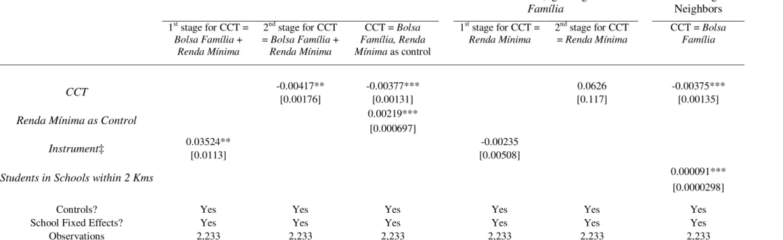
We now address some potential concerns related to our benchmark results. We first analyze whether
incorporating the municipal CCT program (Renda Mínima) affects the results, then consider potential
spillovers of crime across school neighborhoods, and finally address issues related to the functional form of
the estimating equation. In addition, the municipal CCT program allows us to provide some evidence to
validate the exclusion restriction of ourBolsa Famíliainstrument.
As mentioned in section 2, Renda Mínima is a municipal CCT program that sometimes complements
and sometimes replacesBolsa Família. We do not have an institutional change analogous to the expansion of
Bolsa Família coverage that would allow us to estimate an independent causal effect of Renda Mínima.
Therefore, it is not obvious how the municipal CCT program should be incorporated in our analysis. One
alternative would be to sum the total number of children in each school receiving either Bolsa Família or
Renda Mínimato create an aggregate variable for CCT recipients, and then instrument this variable with the
same instrument that we constructed for Bolsa Família. The problem with this procedure would be the
possibility of double counting, since for some families the municipal program complements the federal one.
Another alternative would be simply to include Renda Mínima coverage as an additional control in our
estimation. The problem with this alternative would be thatRenda Mínimasuffers from the same endogeneity
issue discussed before, so that its coefficient – and potentially also the other estimated coefficients – would
be biased. Since there is no clearly dominant strategy between these two, we apply both.
In the first three columns from Table 4, we present the results from these exercises. In the first column,
we present the result from the first stage regression when we consider the sum of recipients ofBolsa Família
and Renda Mínima as the total CCT coverage per school, while in the second column we present the second
before, though the coefficients are estimated slightly less precisely. In the third column, we present the results
when we includeRenda Mínimaas an additional control. Though the coefficient on the municipal CCT appears
as positive and statistically significant, the coefficient on the Bolsa Família variable (instrumented) remains
very similar to what was obtained before. Given our previous discussion on the endogeneity of CCT coverage,
the positive coefficient on Renda Mínimashould be no surprise. The important point from these first three
columns is that, irrespective of how one wants to incorporate Renda Mínima in the estimation, there is no
substantial change on the estimate of the causal impact ofBolsa Famíliaon crime.
But the municipal CCT program also offers an unusual opportunity for us to validate our instrument.
One potential concern is that the initial demographic composition of schools might be correlated with specific
neighborhood characteristics, which, in turn, might be associated with the evolution of socioeconomic
conditions and crime rates over time. If that was the case, our second and first stage results from Tables 2 and
3 would be spurious, reflecting simply the differential dynamic behavior of neighborhoods with a large
number of teenagers around ages 16 and 17. If that was the case, we should expect our strategy to also
deliver similar results when, instead of considering the Bolsa Família program, we consider Renda Mínima.
The latter was not expanded to encompass 16 and 17 year-olds, so our instrument should not work when we
considerRenda Mínima alone and ignoreBolsa Família. If it did work in this setting, this should raise serious
doubts regarding our identification strategy.
In columns 4 and 5 of Table 4 we conduct this exercise. We ignore Bolsa Família coverage and
concentrate solely onRenda Mínima. We then run our most complete specification, corresponding to column
5 in Table 2, and to column 3 in Table 3. Column 4 in Table 4 shows that there is no significant correlation
between our instrument and Renda Mínima coverage. In reality, the point estimate is negative but far from
statistically significant. In column 5, we show that the second stage of this exercise also delivers
non-significant results, which do not carry much meaning anyway given the failure of the first stage. Using our
instrument based on institutional changes to the Bolsa Família CCT program, we are not able to generate
exogenous variation nor to identify any causal effect of the Renda Mínima CCT program, which was not
subject to the same institutional change. These results should be expected if the exclusion restriction implicit
in our instrumental variable approach was met. This indeed seems to be the case.
Another potential concern is related to the geographic dimension of the problem and the possibility of
migration of youth across school neighborhoods. Areas surrounded by a large number of schools with several
students may be subject to more crime because a larger number of students circulate and interact with each
from a given school and including it as an additional control in our benchmark specification. Our variable is the
total number of students in schools within two kilometers of a given school. Column 6 in Table 4 presents the
result of a regression that controls for this additional variable. The point estimate on theBolsa Famíliavariable
(instrumented) remains again very similar to that obtained before. So accounting for the geographic
distribution of schools and the possibility of migration of youths across school neighborhoods makes virtually
no difference to our initial results. Interestingly, we find that the number of students within two kilometers of
a given school has a positive and significant impact on the number of crimes in the school neighborhood. But
the impact is quantitatively very small: a 1 standard deviation increase in the number of students within two
kilometers (5,963) would be associated with 0.5 more crime per year in the school neighborhood.
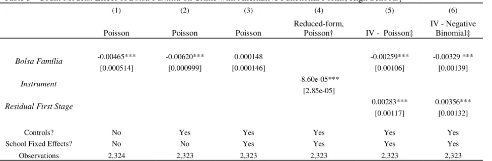
Finally, we address potential concerns related to the functional form of the estimating equation. Our
dependent variable is a non-negative integer, and the number of crimes in some areas is small. Count data
models are arguably more adequate for estimation in this context, where an excessive number of zeros or
over-dispersion may raise specification concerns (Wooldridge, 2002). In our case, when all crimes are
considered, over-dispersion seems to be potentially important, but an excessive number of zeros does not
seem to be an issue (see Figure A.1 in the Appendix).7Still, we re-estimate our benchmark specification using
Poisson and Negative Binomial models. For the case of Poisson, we estimate all specifications corresponding
to columns 1 to 5 in Table 2. For the Negative Binomial, we estimate only specifications corresponding to the
instrumental variable regression from column 5 in Table 2. Given the non-linearity present in all these models,
the instrumental variable strategy is implemented using control functions and standard errors are
bootstrapped.8The coefficients in these count models can be interpreted as semi-elasticities, so that they can
be directly compared to the results obtained before.
The results are displayed in Table 5. The first five columns reproduce the columns from Table 2 using
the Poisson instead of the log-linear model. Qualitative results are identical, though point estimates are a little
different and vary more from specification to specification. Most notably, the results of the simple Poisson
models tend to be larger than the corresponding log-linear specifications, while that of the instrumental
variable strategy is somewhat lower. The last column presents the results when we use the instrumental
variable strategy with the Negative Binomial. The Negative Binomial coefficient, which accounts for
over-7
The average number of crimes around high schools and middle schools is, respectively, 634 and 377. Zeros occur 0.17% and 0.26% of observations in each case.
8
dispersion, is much larger than the corresponding Poisson result, coming closer to the point estimate from
column 5 in Table 2. Overall, issues related to functional forms and count data do not seem to influence the
main results presented before.
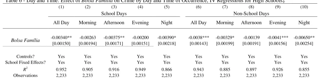
5.3 Channels
The last challenge of this paper is to identify the channels through whichBolsa Famíliaaffects crime. As
mentioned, there are at least three potential channels in this relationship: incapacitation from time spent in
school, income effects from government transfers, and social interactions from changed peer group.
One way to address whether incapacitation seems to be at work is by looking at the effect of Bolsa
Família on crime by day and time of occurrence. Finding larger effects on school days would in principle
suggest an important role for the incapacitation effect, whereby time spent in school “crowds-out”
opportunities for delinquency. We classify each crime in our sample as having occurred on a school or on a
non-school day, corresponding to days with and without classes (non-school days are defined as weekends,
holidays, vacations, etc). We also classify crimes as having occurred in the morning (6:00am-12:00pm),
afternoon (12:00pm-6:00pm), evening (6:00pm-12:00am), and night (12:00am-6:00am). In this classification,
high school classes are typically held in the morning or in the afternoon. Following, we run our benchmark
instrumental variable specification for crimes that occurred in different days and at different times. Results are
presented in Table 6.
The overall effect of Bolsa Família on crime is very similar across school and non-school days, being
even slightly larger for days without classes. This suggests that incapacitation effects are not a relevant
channel behind the impact of CCT on crime. In terms of the hours of occurrence, on days with classes, the
effects ofBolsa Famíliaare concentrated in the afternoon and at night, while there are significant effects in
the morning, evening, and night in days without classes. But coefficients are estimated with less precision
when we look at crimes by time of the day, so one should not attach too much weight to these results. In any
case, no point estimate displays a positive sign, indicating that there is no evidence of a simple displacement
of crime across hours within a day.
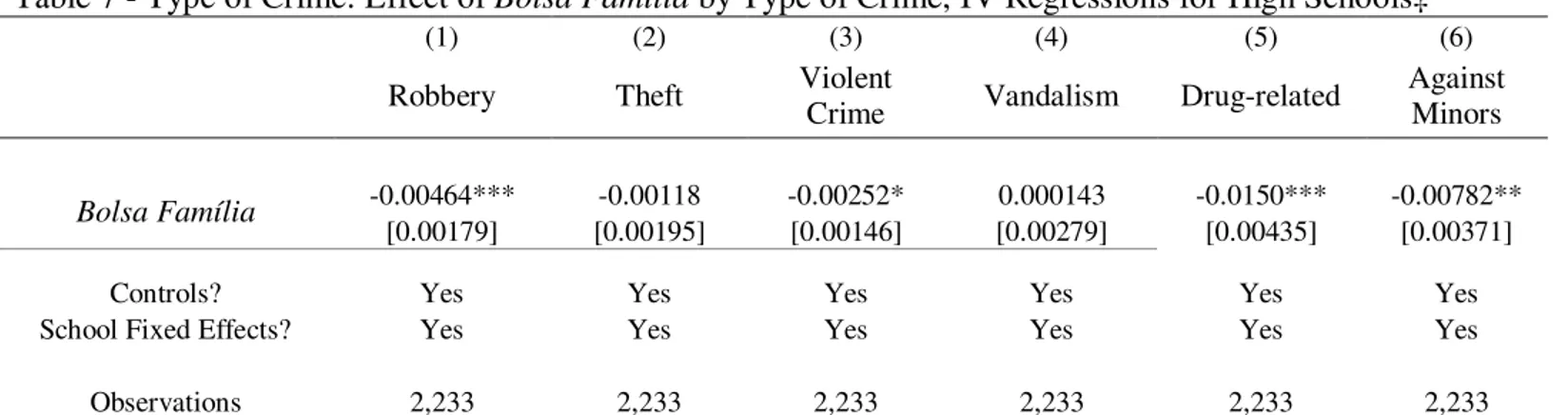
Having ruled out incapacitation as the main channel linking Bolsa Família to crime, we move on to
analyze the impact of the CCT program by type of crime. Types of crimes may reveal whether impacts are
larger in economically motivated crimes, or in more “behavioral” crimes, shedding light on the potential role
of the two remaining mechanisms. We therefore look at the effect of Bolsa Família on robberies, thefts,
The table shows significant negative impacts ofBolsa Famíliaon robberies, drug-related offenses, and
crimes against minors. Thefts are seemingly unaffected, although this category is poorly measured, suffering
from serious underreporting problems (as previously discussed). Point estimates are larger for drug-related
offenses and crimes against minors, but the averages of these crimes are much lower than that of robbery (3
and 5, respectively, against 433). This implies that most of the quantitative impact of the CCT on crime comes
from robberies. There also seems to be a negative correlation betweenBolsa Família and violent crimes, but
the coefficient is much smaller in magnitude and only borderline statistically significant. Overall, the evidence
from the heterogeneous impact of Bolsa Família on different types of crimes suggests that economically
motivated crimes (robberies) are the main driving force in the quantitative response of crime to CCT coverage.
Still, given the evidence on the response of violent crime, drug-related offenses, and crimes against minors,
one cannot entirely rule out some effect through peer groups and social interactions, and even indirect
income impacts through changed household routines, as suggested by Heller et al (2010). Drug-related
offenses are probably a combination of economically motivated and “behavioral” crimes, while violent crimes
are likely to be mostly the latter. Crimes against minors, in turn, are likely to be very sensitive to household
organization and family routines, which may change as a response to increased income.
6. Concluding Remarks
This paper combines detailed crime data from the city of São Paulo with information on Bolsa Família
coverage per school to provide one of the first pieces of evidence on the effect of CCTs on crime. We
overcome the problem of endogeneity of CCT coverage by exploiting an institutional change to the Bolsa
Famíliaprogram that expanded coverage to older age groups. Combining the initial demographic composition
of schools with the timing of institutional change, we construct an instrument that identifies an exogenous
dimension of variation in the number of children covered by the CCT. This instrument allows us to show that
CCT coverage in a school has a negative impact on crime in the neighborhood. The evidence also indicates that
the reduction in crime is not concentrated in school days and seems to be mostly driven by economically
motivated crimes (robberies). So it is likely that the incapacitation effect from time spent in school is not a
particularly relevant mechanism, while the income component of CCTs seems to play an important role.
Our paper speaks directly to the literature on impact evaluations of CCTs by showing that the
reductions in poverty and inequality associated with these programs have broader social consequences, which
should be taken into account in program design and evaluation. Narrow impact evaluations of these
also contribute to the literature on determinants of crime, by presenting an additional piece of evidence on
the relationship between socioeconomic conditions and crime:Bolsa Famíliahas been heralded as an effective
and low cost instrument to fight inequality; our results suggest that the reduction in inequality determined by
the program was accompanied by reduced crime rates, reinforcing the connection between inequality and
crime stressed before in the literature.
References
Anderson, D. Mark (2011). “In School and Out of Trouble? The Minimum Dropout Age and Juvenile Crime.” Unpublished manuscript.
Aizer, Anna (2009). Neighborhood Violence and Urban Youth. In: Jonathan Gruber (ed). The Problems of Disadvantaged Youth – An Economic Perspective. NBER and University of Chicago Press, 2009.
Becker, Gary and Casey B. Mulligan (1997). The Endogenous Determination of Time Preference. Quarterly Journal of Economics, 112(3), 729-58.
Berthelon, Matias E. and Diana I. Kruger (Forthcoming). Risky behavior among youth: Incapacitation effects of school on adolescent motherhood and crime in Chile.Journal of Public Economics, 95 (1-2), 41-53.
Bourguignon, François, Jairo Nuñez, and Fabio Sanchez (2003). A Structural Model of Crime and Inequality in Colombia.Journal of the European Economic Association, 1(2-3), April/May, 440-449.
Cameron, A. Colin and Pravin Triverdi Microeconometrics: Methods and Applications, Cambridge: Cambridge University Press, 2005.
Chamarbagwala, Rubiana and Hilcías E. Morán (2011). The human capital consequences of civil war: Evidence from Guatemala.Journal of Development Economics, 94(1), 41-61.
DeFranzo, James (1996). Welfare and Burglary.Crime and Delinquency, 42, 223-229.
DeFranzo, James (1997). Welfare and Homicide.Journal of Research in Crime and Delinquency, 34, 395-406.
Dobkin, Carlos and Stephen Puller (2007). The Effects of Government Transfers on Monthly Cycles in Drug Abuse, Hospitalization, and Mortality.Journal of Public Economics, 91(11-12), 2137-57.
Fajnzylber, Pablo, Daniel Lederman, and Norman Loayza (2002). Inequality and violent crime. Journal of Law and Economics, April 2002, 45(1), 1-40.
Fiszbein, Ariel and Norbert Schady (2009). Conditional Cash Transfers: Reducing Present and Future Poverty. World Bank, Washington DC.
Foley, C. Fritz (2008). “Welfare Payments and Crime.” NBER Working Paper 14074.
Gottfredson, Denise C. and David A. Soulé (2005). The Timing of Property Crime, Violent Crime, and Substance Use among Juveniles.Journal of Research in Crime and Delinquency, 42(110), 110-120.
Gould, Eric D., Bruce A. Weinberg, and David B. Mustard (2002). Crime Rates and Local Labor Market Opportunities in the United States: 1979-1997.Review of Economics and Statistics, 84(1), 45-61.
Hannon, Lance, and James DeFranzo (1998). Welfare and Property Crime.Justice Quarterly, 15, 273-287.
Heller, Sara B., Brian A. Jacob and Jens Ludwig (2011). Family Income, Neighborhood Poverty, and Crime. In: P. Cook, J. Ludwig and J. McCrary (eds.), Controlling Crime: Strategies and Tradeoffs, University of Chicago Press, 419-459.
Jacob, Brian A. and Lars Lefgren (2003). Are Idle Hands the Devil’s Workshop? Incapacitation, Concentration, and Juvenile Crime.American Economic Review, 93(5), 1560-1577.
Jacob, Brian A. and Jens Ludwig (2010). The Effects of Family Resources on Children’s Outcomes. Working Paper, University of Michigan.
Levitt, Steven D. and Lance Lochner (2001). The Determinants of Juvenile Crime. In: J. Gruber (ed.), Risky Behavior among Youths: An Economic Analysis, University of Chicago Press, 327-373.
Lochner, Lance and Enrico Moretti (2004). The Effect of Education on Crime: Evidence from Prison Inmates, Arrests, and Self-Reports.American Economic Review, 94(1), 155-189.
Lochner, Lance (2010). “Education Policy and Crime.” NBER Working Paper 15894.
Loureiro, André (2012). “Can Conditional Cash Transfers Reduce Crime? Evidence from Brazil.” Unpublished manuscript.
Luallen, Jeremy (2006). School’s out. . . forever: A study of juvenile crime, at-risk youths and teacher strikes. Journal of Urban Economics, 59(1), 75–103.
Rodríguez, Catherine and Fabio Sánchez (2009). “Armed Conflict Exposure, Human Capital Investments and Child Labor: Evidence from Colombia.” Serie Documentos CEDE 2009-05, Universidad de Los Andes.
Snyder, Howard N. and Melissa Sickmund (1999). Juvenile Offenders and Victims: 1999 National Report. US Department of Justice Programs, Office of Juvenile Justice and Delinquency Prevention, Washington DC.
Soares, Rodrigo R. (2004). Development, crime, and punishment: Accounting for the international differences in crime rates.Journal of Development Economics, 73(1), 155-184.
Soares, Rodrigo R. and Joana Naritomi (2010). Understanding High Crime Rates in Latin America: The Role of Social and Policy Factors. In: Rafael Di Tella, Sebastian Edwards, and Ernesto Schargrodsky (eds). The Economics of Crime: Lessons for and from Latin America, University of Chicago Press, 2010, 19-55.
Soares, Sergei and Natália Sátyro (2009). “O Programa Bolsa Família: Desenho Institucional, Impactos e Possibilidades Futuras.” IPEA Working Paper n1424.
Wooldridge, Jeffrey (2002).Econometric Analysis of Cross Section and Panel Data, MIT Press.
APPENDIX A
Figure A.1 - Distribution of Number of Crimes per School
0
.1
.2
.3
.4
P
e
rc
e
n
t
0 5000 10000
Panel A : Unconditional
Histogram of All Crimes
0
5
1
0
1
5
P
e
rc
e
n
t
0 10 20 30
Panel B : Conditional on less than 200 occurences
Histogram of All Crimes
Table 1 - Summary Statistics:Bolsa Famíliaand Crime
Panel A: Middle Schools
Mean Std Deviation
25th
percentile Median
75th percentile
#
Schools # Obs
All Crimes 377 561 132 240 408 975 3900
% 16-17 in 2006 15% 13% 3% 13% 27% 975 975
# receivingBolsa Família 166 115 82 139 220 975 3900
# students 1248 457 899 1194 1564 975 3900
Panel B: High Schools
Mean Std Deviation
25th
percentile Median
75th percentile
#
Schools # Obs
All Crimes 634 761 235 447 767 581 2324
% 16-17 in 2006 28% 11% 20% 28% 33% 581 581
# receivingBolsa Família 124 95 57 102 170 581 2324
# students 1360 499 853 1345 1721 581 2324
Panel C: Middle and High
Schools Together Mean Std
Deviation
25th
percentile Median
75th percentile
#
Schools # Obs
All crimes reported 356 521 125 230 395 1035 4140
% 16-17 in 2006 17% 15% 3% 15% 30% 1035 1035
# receivingBolsa Família 162 116 79 135 216 1035 4140
# students 1251 457 898 1194 1567 1035 4140
Table 2 - Main Estimates: Effect ofBolsa Famíliaon All Crimes
Panel A: Middle Schools (1) (2) (3) (4) (5)
OLS OLS OLS
Reduced-form† IV‡
Bolsa Família -0.00224*** -0.00157*** 5.04e-05 -0.000920***
[0.000254] [0.000296] [0.000234] [0.000290]
Instrument -0.000129***
[4.64e-05]
Controls? No Yes Yes Yes Yes
School Fixed Effects? No No Yes Yes Yes
R2 0.062 0.165 0.949 0.949
Observations 3,900 3,726 3,726 3,726 3,726
Panel B: High Schools (1) (2) (3) (4) (5)
OLS OLS OLS
Reduced-form† IV‡
Bolsa Família -0.00396*** -0.00384*** 6.46e-05 -0.00391***
[0.000419] [0.000506] [0.000276] [0.00141]
Instrument -0.000147***
[5.53e-05]
Controls? No Yes Yes Yes Yes
School Fixed Effects? No No Yes Yes Yes
R2 0.130 0.334 0.967 0.967
Observations 2,324 2,233 2,233 2,233 2,233
Panel C: Middle and High Schools Together
(1) (2) (3) (4) (5)
OLS OLS OLS
Reduced-form† IV‡
Bolsa Família -0.00235*** -0.00147*** 3.67e-05 -0.00110***
[0.000247] [0.000281] [0.000221] [0.000284]
Instrument -0.000133***
[3.90e-05]
Controls? No Yes Yes Yes Yes
School Fixed Effects? No No Yes Yes Yes
R2 0.068 0.196 0.949 0.949 0.947
Observations 4,140 3,958 3,958 3,958 3,958
Table 3 - First Stage:Bolsa FamíliaRegressed on Instrument, High Schools
(1) (2) (3)
Instrument‡ -0.0103 0.0174** 0.0376***
[0.0163] [0.00823] [0.00782]
Controls? No No Yes
School Fixed Effects? No Yes Yes
R2 0.084 0.912 0.925
F-statistic of Instrument 0.401 4.467 23.10
Observations 2,324 2,324 2,233
Source: Standard errors in parentheses robust to clustering at the school level. * significant at 10%; ** significant at
5%; *** significant at 1%. Unit of observation is a school. Dependent variable is the number ofBolsa Família
Table 4 - IncorporatingRenda Mínimaand Neighboring Schools: Effect ofCCTon Crime, High Schools
(1) (2) (3) (4) (5) (6)
Bolsa FamíliaandRenda Mínima Renda Mínima, ignoringBolsa Família
Accounting for Neighbors
1ststage for CCT =
Bolsa Família+
Renda Mínima
2ndstage for CCT =Bolsa Família+
Renda Mínima
CCT =Bolsa Família, Renda Mínimaas control
1ststage for CCT =
Renda Mínima
2ndstage for CCT =Renda Mínima
CCT =Bolsa Família
CCT -0.00417** -0.00377*** 0.0626 -0.00375***
[0.00176] [0.00131] [0.117] [0.00135]
Renda Mínima as Control 0.00219***
[0.000697]
Instrument‡ 0.03524** -0.00235
[0.0113] [0.00508]
Students in Schools within 2 Kms 0.000091***
[0.0000298]
Controls? Yes Yes Yes Yes Yes Yes
School Fixed Effects? Yes Yes Yes Yes Yes Yes
Observations 2,233 2,233 2,233 2,233 2,233 2,233
Table 5 - Count Models: Effect ofBolsa Famíliaon Crime with Alternative Functional Forms, High Schools‡
(1) (2) (3) (4) (5) (6)
Poisson Poisson Poisson
Reduced-form,
Poisson† IV - Poisson‡
IV - Negative Binomial‡
Bolsa Família -0.00465*** -0.00620*** 0.000148 -0.00259*** -0.00329 ***
[0.000514] [0.000999] [0.000146] [0.00106] [0.00139]
Instrument -8.60e-05***
[2.85e-05]
Residual First Stage 0.00283*** 0.00356***
[0.00117] [0.00132]
Controls? No Yes Yes Yes Yes Yes
School Fixed Effects? No No Yes Yes Yes Yes
Observations 2,324 2,323 2,323 2,323 2,323 2,323
Table 6 - Day and Time: Effect ofBolsa Famíliaon Crime by Day and Time of Occurrence, IV Regressions for High Schools‡
(1) (2) (3) (4) (5) (6) (7) (8) (9) (10)
School Days Non-School Days
All Day Morning Afternoon Evening Night All Day Morning Afternoon Evening Night
Bolsa Família -0.00340** -0.00263 -0.00375** -0.00200 -0.00390* -0.0038*** -0.00329* -0.00139 -0.0041*** -0.00650**
[0.00150] [0.00194] [0.00171] [0.00151] [0.00218] [0.00143] [0.00199] [0.00191] [0.00156] [0.00254]
Controls? Yes Yes Yes Yes Yes Yes Yes Yes Yes Yes
School Fixed Effects? Yes Yes Yes Yes Yes Yes Yes Yes Yes Yes
R2 0.952 0.905 0.916 0.949 0.866 0.943 0.885 0.897 0.926 0.855
Observations 2,233 2,233 2,233 2,233 2,233 2,233 2,233 2,233 2,233 2,233
Table 7 - Type of Crime: Effect ofBolsa Famíliaby Type of Crime, IV Regressions for High Schools‡
(1) (2) (3) (4) (5) (6)
Robbery Theft Violent
Crime Vandalism Drug-related
Against Minors
Bolsa Família -0.00464*** -0.00118 -0.00252* 0.000143 -0.0150*** -0.00782**
[0.00179] [0.00195] [0.00146] [0.00279] [0.00435] [0.00371]
Controls? Yes Yes Yes Yes Yes Yes
School Fixed Effects? Yes Yes Yes Yes Yes Yes
Observations 2,233 2,233 2,233 2,233 2,233 2,233