Repositório Institucional UFC: Comparative study between PI-AW and MPC controllers with Gaussian noise in feedback loop

(1)

CENTRO DE TECNOLOGIA

DEPARTAMENTO DE ENGENHARIA ELÉTRICA

PROGRAMA DE PÓS-GRADUAÇÃO EM ENGENHARIA ELÉTRICA MESTRADO ACADÊMICO EM ENGENHARIA ELÉTRICA

MISAEL FELIX QUISPE MAIDANA

COMPARATIVE STUDY BETWEEN PI-AW AND MPC CONTROLLERS WITH GAUSSIAN NOISE IN FEEDBACK LOOP

(2)

COMPARATIVE STUDY BETWEEN PI-AW AND MPC CONTROLLERS WITH

GAUSSIAN NOISE IN FEEDBACK LOOP

Dissertação apresentada ao Curso de Mes-trado Acadêmico em Engenharia Elétrica do Programa de Pós-Graduação em engenharia Elétrica do Centro de Tecnologia da Universi-dade Federal do Ceará, como requisito parcial à obtenção do título de mestre em Engenharia Eléctrica. Área de Concentração: Engenharia Elétrica

Orientador: Prof. Dr. Wilkley Bezerra Correia

Coorientador: Prof. Dr. Bismark Claure Torrico

FORTALEZA

(3)

Gerada automaticamente pelo módulo Catalog, mediante os dados fornecidos pelo(a) autor(a)

M189c Maidana, Misael Felix Quispe.

Comparative study between PI-AW and MPC controllers with Gaussian noise in feedback loop / Misael Felix Quispe Maidana. – 2018.

75 f. : il. color.

Dissertação (mestrado) – Universidade Federal do Ceará, Centro de Tecnologia, Programa de Pós-Graduação em Engenharia Elétrica, Fortaleza, 2018.

Orientação: Prof. Dr. Wilkley Bezerra Correia. Coorientação: Prof. Dr. Bismark Claure Torrico.

1. Ruído. 2. Saturação. I. Título.

(4)

COMPARATIVE STUDY BETWEEN PI-AW AND MPC CONTROLLERS WITH GAUSSIAN NOISE IN FEEDBACK LOOP

Dissertação apresentada ao Curso de Mes-trado Acadêmico em Engenharia Elétrica do Programa de Pós-Graduação em engenharia Elétrica do Centro de Tecnologia da Universi-dade Federal do Ceará, como requisito parcial à obtenção do título de mestre em Engenharia Eléctrica. Área de Concentração: Engenharia Elétrica

Aprovada em: 28 de Março de 2018

BANCA EXAMINADORA

Prof. Dr. Wilkley Bezerra Correia (Orientador) Universidade Federal do Ceará (UFC)

Prof. Dr. Bismark Claure Torrico (Coorientador) Universidade Federal do Ceará (UFC)

Prof. Dr. Fabrício Gonzalez Nogueira Universidade Federal do Ceará (UFC)

(5)

(6)

I would like to express my deep gratitude to Professor Wikley and Professor Bis-mark, my research supervisors, for their patient guidance, enthusiastic encouragement and use-ful critiques of this research work. I want also like to thank Professor Laurinda and Fabricio, for their advice and assistance in keeping my progress on schedule.

I would also like to extend my thanks to all the Group of Brazilian universities

COIMBRAand the Capes Foundation, for trusting on me for the realization of this specialization at the Federal University of Ceará.

(7)

tries.”

(8)

O presente trabalho propõe um estudo comparativo entre o controlador PI clássico com estrutura Anti-Windup (PI-AW) e Controle Preditivo basado em Modelo (MPC), ou seja, o controlador GPC-T. Estas duas técnicas de controle são aplicadas em diferentes plantas, considerando as seguintes situações: Presença de saturação no sinal de controle, o qual está relacionado às limitações físicas dos atuadores e à presença de ruído Gaussiano no laço de realimentação. Fi-nalmente, como é bem conhecido no controle do processos, os atuadores geralmente operam perto de seus limites de saturação, por exemplo, o controle de velocidade de um motor elétrico está sempre sob a influência da carga, pois o sinal de controle conduz os atuadores próximos aos seus limites de operação. Portanto, tem-se perda de referência levando a um erro de es-tado estacionário, o que é indesejável nos processos de controle. Este é o fenômeno Erro de

Rastreamento Induzido por RuídoNITE.

Embora o controlador preditivo GPC tem mostrado um desempenho menor em comparação com o PI-AW, incorporação o polinômio-T, o seja o conhecido controlador GPC-T melhorou consideravelmente a rejeição de perturbações e a atenuação do ruído, quando a saturação é incluída no processo de otimização com restrição, então se diminui o fenômeno NITE.

Para verificar experimentalmente a análise mencionada encima, tem sido escolhido o laço de controle de velocidade de um Motor de Relutância Variável (MRV). Essa planta mostrou ser adequada para a análise, pois possui oscilações mecânicas intrínsecas e o ruído de medição. Portanto, ao escolher corretamente uma velocidade de referência, pode-se levar a máquina a operar muito perto dos limites dos atuadores, enfatizando o efeito de distúrbios e ruídos na operação geral. Então o fenômeno NITE é verificado e sua diminuição pelo controlador GPC-T com otimização analítica para diminuir o esforço computacional no DSP.

(9)

The present work proposes a comparative study between the classical PI controller with Anti-windup structure (PI-AW) and a Model Predictive Control (MPC), then the control to be applied is GPC-T. These two control techniques are applied to different plants considering the following situations: Presence of saturation on the control signal, which is related to the real limitations of actuators and the Gaussian noise presence in the feedback loop. Finally, as it is well known in the process control, actuators commonly operate close to their saturation limits, e.g., speed control of an electric motor is always under the influence of the load as consequence the control signal leads the actuators close to their limits. Therefore, loss of reference may happen leading to a steady-state error, which is undesirable in the control processes. This phenomenon is called

Noise Induced Tracking ErrorNITE.

Although predictive controller GPC has shown poorer performance compared to the PI-AW one, incorporation of the T-polynomial, i.e., the well-known GPC-T controller considerably improved both disturbance rejection and noise attenuation, when saturation is included in the optimization process with constraint, i.e, decreases the NITE phenomenon.

In order to verify the aforementioned analysis experimentally, it has been chosen the speed control loop of a variable reluctance motor (SRM). Such plant has been shown to be suitable for the analysis as it has intrinsic mechanical oscillations and measurement noise. Therefore, by properly choosing a reference speed, one may take the machine to operate very close to the actuators limits, emphasizing the disturbances effect and noises in the overall operation. Then the NITE phenomenon is verified and its decrease by the GPC-T controller with analytic optimization, to decrease the computational effort in the DSP.

(10)

Figure 1 – Limitation in the amplitude of control signal. . . 21

Figure 2 – Control loop block diagram. . . 22

Figure 3 – Windup effect response. . . 22

Figure 4 – PI controller with saturation. . . 23

Figure 5 – System response Y(s). . . 23

Figure 6 – Control signal ˆu. . . 24

Figure 7 – Behavior of integral term I. . . 24

Figure 8 – Different types of noise. . . 25

Figure 9 – Gaussian noise probability function . . . 26

Figure 10 – PI-AW controller with noise in feedback loop. . . 27

Figure 11 – System response without noise . . . 27

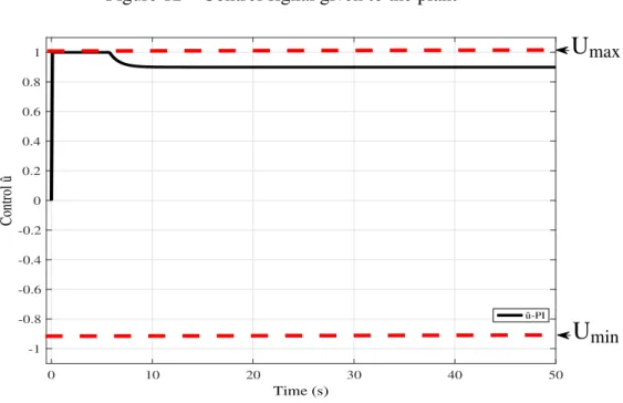
Figure 12 – Control signal given to the plant . . . 28

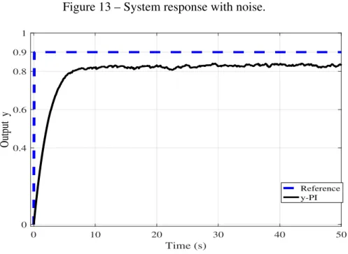
Figure 13 – System response with noise. . . 29

Figure 14 – control signal given to the plant. . . 29

Figure 15 – Structure of the PI controller. . . 30

Figure 16 – Proportional control action. . . 31

Figure 17 – Integral control action. . . 32

Figure 18 – Structure of PI-AW controller technique Tracking Mode. . . 34

Figure 19 – Classical RST structure applied to SRM speed control. . . 42

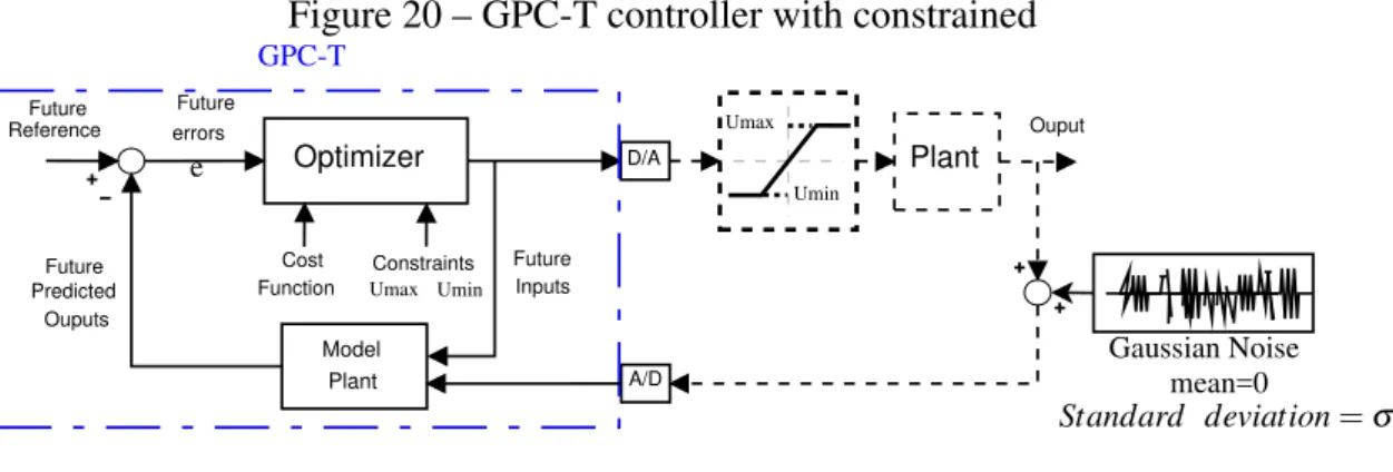
Figure 20 – GPC-T controller with constrained . . . 45

Figure 21 – Comparison structure of the PI-AW and GPC-T controllers . . . 47

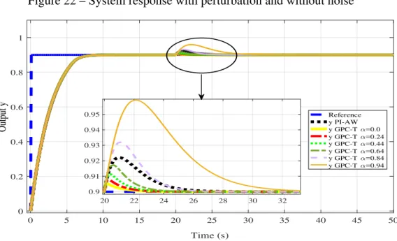
Figure 22 – System response with perturbation and without noise . . . 48

Figure 23 – Control signal ˆu after saturator . . . 49

Figure 24 – System response with Gaussian noise (σ=0.1) . . . 50

Figure 26 – System response with perturbation and without noise . . . 53

Figure 28 – System response with Gaussian noise (σ=5) . . . 54

Figure 30 – New Land Rover 2013 all-electric with motor SRM 4x4 . . . 57

(11)

Figure 33 – Structure physical of SRM. . . 58

Figure 34 – Asymmetric Bridge Converter and SRM . . . 59

Figure 35 – Overall block diagram of speed loop . . . 60

Figure 36 – Schematic behavior of the main SRM variables . . . 61

Figure 37 – Structure of SRM controller . . . 61

Figure 38 – Test prototype of SRM speed controller. . . 61

Figure 39 – Overall block diagram of identification SRM of the speed loop . . . 62

Figure 40 – Simulated response of SRM speed control . . . 64

Figure 41 – Simulated control signal ˆu . . . 64

Figure 42 – Experimental response of SRM speed control . . . 65

Figure 43 – Experimental control signal ˆu . . . 65

Figure 44 – Simulated response of SRM speed control (α _→1) . . . 66

Figure 45 – Simulated control signal ˆu (α _→1) . . . 66

Figure 46 – Experimental response of SRM speed control (α _→1) . . . 67

(12)

Table 1 – Performance indices without noise for stable plant . . . 49

Table 2 – Performance indices with noise for stable plant . . . 52

Table 3 – Performance indices without noise for integral plant . . . 54

Table 4 – Performance indices with noise for integral plant . . . 55

Table 5 – Physical parameters of SRM used . . . 58

(13)

CARIMA Auto Regressive Integrated Moving Average DSP Digital Signal Processor

GPC Generalized Predictive Control IAE Integral Absolute Error

MPC Model Predictive Control NITE Noise Induced Tracking Error PI Proportional Integral

PID Proportional Integral Derivative PWM Pulse Width Modulation

SISO Single Input Single Output

(14)

∆ discrete-time integrator

∆u(t) control weighting

ε hysteresis width

λ control weighting

ω_m angular velocity

θ rotor position

d transportation delay

θ_{o f f} disconnection angle

θ_on shooting angle

f free answer of the system

Gpv speed plant model

in phase current

Ire f reference current

Kp proportional gain

Ki integral gain

Ka gain action of mitigate windup

N Prediction horizon;

N₁ minimum prediction horizon

N2 maximum prediction horizon

Nu control horizon

n(t) noise signal P(s) plant model Ts sampling time

t time

u(t) control signal

(15)

y output signal

zc position of zero controller

(16)

1 INTRODUCTION . . . 17

1.1 Motivation . . . 18

1.2 Objetives . . . 19

1.2.1 Overall objective . . . 19

1.2.2 Specific objectives . . . 19

1.3 Scientific Production . . . 19

1.4 Thesis Overview . . . 19

2 INFLUENCE FACTORS IN THE CONTROL LOOPS . . . 21

2.1 Windup effect . . . 21

2.2 Noise in the Process. . . 25

3 CONTROLLERS DESIGNS . . . 30

3.1 Proportional Integral Control . . . 30

3.1.1 PI Control Structure . . . 30

3.1.2 Controller adjustment methods . . . 32

3.1.2.1 Root Locus Method . . . 32

3.1.3 Anti-Windup PI . . . 34

3.2 Model Predictive Control . . . 35

3.2.1 GPC Controller . . . 35

3.2.1.1 Unconstrained optimization . . . 40

3.2.1.2 Constrained optimization . . . 43

3.3 Performance Indices . . . 45

4 CASE STUDIES . . . 47

4.1 Stable process . . . 48

4.2 Integral process . . . 52

4.3 Switched Reluctance Motor . . . 56

4.3.1 Description of the test prototype . . . 57

4.3.1.1 Physical principle of operation SRM . . . 58

4.3.1.2 Asymmetric Bridge Converter . . . 59

4.3.1.3 Complete diagram of the prototype . . . 59

4.3.2 Modelling of the SRM. . . 62

(17)

4.3.3.1 Results . . . 63

5 CONCLUSION AND FUTURE WORK . . . 69

5.1 Conclusion . . . 69

5.2 Future work . . . 70

(18)

1 INTRODUCTION

Currently, in the industrial environment, it is very common the need of controllers with easy operation and simple adjustment. Therefore, the control engineering has involved the development of methods and techniques that are constantly evolving in order to improve performance, efficiency and effectiveness in the control loop (NUNES, 2001).

Since its introduction the Proportional-Integral-Derivative PID controller has been by far the most extensively controller for industrial applications (ASTRöM; HäGGLUND, 1995). Its success is mainly due to its simple structure and ease parameters tuning for a wide range of different real processes.

Many processes may present failures in system performance which usually cannot be predicted. These failures are derived of certain restrictions to which most industrial processes are subjected or under certain specific working circumstances, but these are not considered during the design of the controllers.

In real processes there are usually physical limitations by part of the actuators, these are responsible for translating the control signal granted by the control law to run it on the plant. Few examples include industrial communication between control equipment and final actuators, which commonly use the HART (Highway Addressable Remote Transducer) protocol, that only operates in the current range of 4 to 20mA(GUERREROet al., 2009). A solenoid valve cannot open more than 100% and a motor cannot work beyond the rated speed. These limitations may be named saturation (VISIOLI, 2006).

The actuator saturation is the most common and significant of the non-linearity found in control system. In the literature, there are several examples where by neglecting them the saturation has led to crucial difficulties and put in danger the overall stability of the system. For example, it has also been blamed as one of several unfortunate mishaps leading to the 1986 Chernobyl nuclear power plant disaster where unit 4 melted down with dreadful consequences (STEIN, 1989; KOTHARE, 1997).

(19)

(OGATA, 1997).

The noise is present in the physical processes, which tends to be of a higher fre-quency with relation to process dynamics. Sources of signal noise are due to: Electrical inter-ference, Jitter (clock related irregularities such as variations in sample spacing), quantifying of signal samples into overly-broad discrete “buckets” from low resolution or improperly specified instrumentation (e.g. too-large measurement span relative to operating range), vibrations of the actuators (bad adjustment of equipment) or the same plant to be controlled presents vibrations (KIMet al., 2015), (MOHAMMED, 2017).

1.1 Motivation

In the study of the classical control technique PI-AW, recently it was mentioned for a stable plant in open loop by (EUN; S., 2015), when there is the presence of Gaussian noise in the feedback loop and saturation of the control signal. These characteristics induce the loss of reference tracking, consequently, there is a steady-state error. This phenomenon is calledNoise

Induced Tracking Error NITE by (EUN; S., 2015). Later also it was analyzed for different types anti-windup structures with PI controller, where show thatNITEphenomenon occurs by (LEE; EUN, 2016).

For the mentioned, it is observed that the tuning parameters of the PI-AW con-troller are not appropriate, therefore to correct the phenomenon is necessary to readjust of the controller parameters to eliminate this phenomenon NITE. However, this process changes the projected response of system and it is not industrially desired because time-consuming requires as well as the discontinuity of process in question.

The hypothesis is if this phenomenon NITE can occur in other controllers. Then the Model Predictive Control MPC will be studied, because is an advanced method of pro-cess control that is used to control a multi-input, multi-output propro-cess while satisfying a set of constraints. It has been in use in the process industries in energy generation, ship build-ing, chemical plants and oil refineries since the 1980 (ALLGöWER; ZHENG, 2000). In re-cent years it has also been used in power system balancing models and in power electronics (SHORT; ABUGCHEMN, 2017).

(20)

1.2 Objetives

In view of the exposed in the previous section, it develops the overall objective and Specific objectives to achieve in the present thesis.

1.2.1 Overall objective

The objective is to perform a comparative study of performance of the PI-AW and MPC controllers to different plants: stable, integrative, SRM, under the presence of noise in feedback loop. For the design of the controller MPC it applies the GPC controller which will incorporate the application of the T-polynomial to reject step-like disturbances and noise atten-uation, i.e., a GPC-T controller.

1.2.2 Specific objectives

• Review of control strategy PI-AW and GPC-T.

• To perform simulations of the designed controllers applied the presence of noise in the feedback loop.

• To implement control techniques studied in the control of speed of the SRM. • Compare performance of controllers, through the performance indicesIAE,TV.

1.3 Scientific Production

Throughout the development of this thesis was published the article:

Maidana,M.Q. & Correia,B.W. & Torrico, B.C. & Nogueira,F.G., "Comparative study of PI-AW and MPC-T controllers, with feedback noise applied for speed control to a Switched Reluctance Motor (SRM)", accepted in Brazilian Power Electronics Conference (COBEP-2017)

1.4 Thesis Overview

In order to present the developed aspects throughout the research, this thesis it was divided into 5 Chapters including this introduction, then is organized as follows:

• Chapter 2:

(21)

and the noise measurement.

• Chapter 3

This chapter is divided into three subsections:

First place, to review of the classic controller PI with Anti-Windup structure, i.e., a PI-AW. Second place, it is a review of the MPC control structure from which it decomposes the Generalized Predictive Controller (GPC). Finally, cite the definitions of the performance indicesIAEandTV.

• Chapter 4

This chapter is divided into two sections:

First place, compare the PI-AW and GPC-T controllers for the stable and integral plant in form of simulations. Second place has been validated the comparison of the PI-AW and GPC-T controllers experimentally through the speed control of a Switch Reluctance Motor (SRM). So these analyzes are validated by performance indices.

• Chapter 5:

(22)

2 INFLUENCE FACTORS IN THE CONTROL LOOPS

This chapter discusses two influence factors recurring in the process control loops, such as internal (Windup) and external (noise measurement), whose influence may vary depend-ing upon the process. The Windup effect is studied is many associated with the integral action due the controller and saturation for the control signal. Then the presence of noise measurement in the feedback loop is highlighted. Finally, an example is discussed for a stable plant with PI controller with Anti-windup effect, i.e., a PI-AW controller. It also contemplates the presence of Gaussian noise present in the feedback loop, so one can observe this particular phenomenon.

2.1 Windup effect

One of the most commonly neglected and often undetected problems in control loop is the wind-up effect. This occurs when a controller with integral action exceeds the physical limits of the actuator. In this work, only the amplitude limitation is considered in the actuator, which is quite common, being described by the following nonlinear function:

ˆu=sat(u) =

      

     

Umin i f u<Umin

u i f Umin≤u≤Umax

Umax i f u>Umax

, (2.1)

where Uminand Umax are the minimum and maximum signals allowed by the actuator. It can be represented as in Figure 1.

Figure 1 – Limitation in the amplitude of control signal.

Controller Process

u û

Actuator

U

max

U

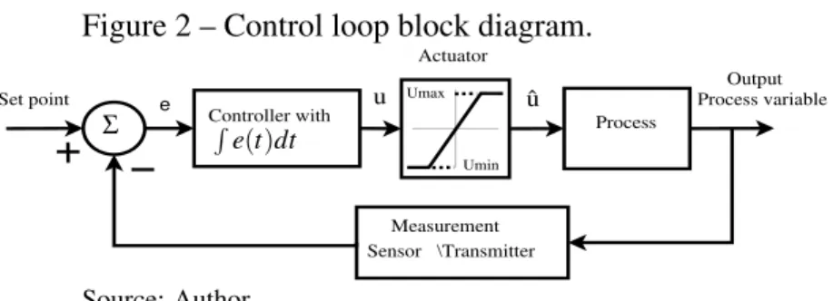
min Source: Author.

(23)

Figure 2 – Control loop block diagram.

Controller with

Sensor Set point

Output

Process

Measurement \Transmitter

Process variable Umax

Umin

u û

Actuator

e

R e(t)dt

Σ

Source: Author

If the set point receives a sudden positive step command, the error, e, will initially be positive as the system begins to respond to the actuator. If the rate of integration is fast with respect to the speed of the system, the integrator output may exceed the saturation limit of the actuator but continue to grow in size itself (see Figure 3 Integral control action). When the system output finally reaches the commanded value, the sign of the error reverses causing the integrator to begin "winding" down. But the output of the integrator, far beyond the operating range of the actuator, takes such a significant amount of time to recover within the operating range of the actuator and so causes a lag in response. This process can repeat itself as a limit cycle, or eventually converge towards the commanded value depending on the set gain and system response (DORF; BISHOP, 2011).

Figure 3 – Windup effect response.

Setpoint _Process

variable

Maximum control

effort

Control effort

Time Time u

Source: (DORF; BISHOP, 2011)

The Windup effect can occur in electronic, mechanical or software components in a control loop. It may also occur in any control element that contains memory. A first-order lag or any filter can create Windup. If the designer permits Windup to occur, the closed loop system can exhibit excessive overshoot, sustained oscillations, and/or lengthy settling times (HU; LIN, 2001a). Finally, overshoot may be due to a dominating possession of zero that has the process.

(24)

for a PI controller (see Figure 4).

Figure 4 – PI controller with saturation.

P(s) Kp

Ki 1/s

Y(s)

R(s) _e Umax

Umin

u

û

Actuator

I(s) Σ Σ

Source: Author

Where the chosen plant isP(s) =₍₃_s1₊₁₎and the controller is tuned asKp=5,Ki=3.

The control signal delivered to the saturator is given by:

u(t) =Kpe(t) +Ki

Z t

0 e(t)dt, (2.2)

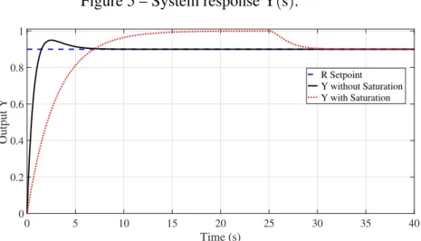
then when signal u passes through the saturator (see Equation ( 2.1)), signal ˆu is delivered to the process, whose graphs are given in the Figures 5, 6, 7.

Figure 5 – System response Y(s).

0 5 10 15 20 25 30 35 40

Time (s)

0 0.2 0.4 0.6 0.8 1

Output Y

R Setpoint Y without Saturation Y with Saturation

(25)

Figure 6 – Control signal ˆu.

0 5 10 15 20 25 30 35 40

Time (s) -1 -0.5 0 0.5 1 1.5 2 2.5 3 3.5 4

Control signal û

Umax Umin

û=u without Saturation û with Saturation

0 5 10 15 20 25 30 35

0.85 0.9 0.95 1

Source: Author

Figure 7 – Behavior of integral term I.

0 5 10 15 20 25 30 35 40

Time (s) 0 1 2 3 4 5 6 Integral Term

I without Saturation I with Saturation

Source: Author

As shown in the Figure 7 there is an overshot (red color), which is due to the integral action of the PI controller, this is the Windup effect.

Very often a design will look good in simulation or on paper, but when implemented fails to perform as expected. Unknowingly, the designer will attempt to fix the problem by reducing gains of the controller. This slows integration rates to match the system speed and can prevent Windup in the closed loop, but at the expensive of reduced speed of the closed loop response (OGAWAet al., 2010).

(26)

A classic solution to the phenomenon windup is known as Anti-Windup is known as back-calculation, tracking, or classical Anti-Windup. The method was first described by (FERTIK; ROSS, 1967). This Anti-Windup algorithm is detailed in chapter 3 of this thesis.

2.2 Noise in the Process

Noise may be seen as any unwanted high-frequency signal that is added in the feed-back loop. There are multiple sources of noise, some external as a motor of a car, elevator, mo-bile phone, etc. and others internal as thermal noise, parts wear, etc. (HANSLER; SCHMIDT, 2004).

In an industrial plant by the conditions physical existing the noise is present, there-fore must be considered its effects in the controller design. The nature of noise sources is random for which it is suitable to consider a stochastic approach. Within this context, one may highlight (HANSLER; SCHMIDT, 2004):

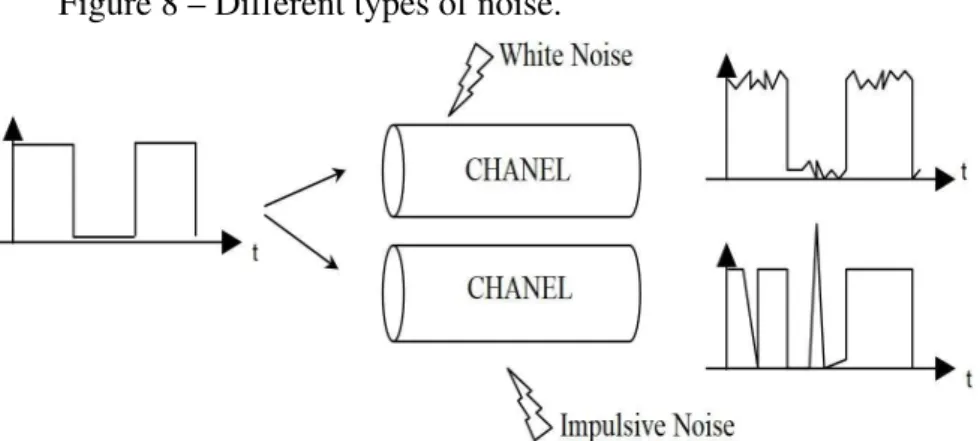
• White noise where its energy density is distributed equally in all the frequency range. Example: Thermal noise caused by a random motion of the electrons of a metal with the temperature (see Figure 8).

• Impulsive Noise, which is mainly produced at irregular intervals with very pronounced peaks of short duration. Usually has external origin as: lighting of a light, relays, etc. (see Figure 8).

Figure 8 – Different types of noise.

Source: <http://trajano.us.es/~rafa/ARSS/apuntes>

(27)

So the white noise is a Gaussian noise (see Figure 9), then it begins with determin-ing the likely values of statistics measures that character the level of noises in the system (LI, 2005). It is well known that the probability of a Gaussian random variableX fall in the interval

[mx−a,mx+a]is:

P[mx−a≤X≤mx+a] =er f

a √

2σ_x

, (2.3)

wheremx is the mean, andσx2 is the variance ander f(.)is the error function (also

called the Gauss error function) is a special function (non-elementary) of sigmoid shape that occurs in probability, statistics, and partial differential equations describing diffusion. It is defined as:

er f(x) = √2

π

Z x

0 e

−t2_dt_, _(2.4)

in statistics for non negative values ofx, the error function has the following interpretation: for a random variable Y that is normally distributed with mean 0 and variance 1/2,er f(x)describes the probability ofY falling in the range[₋x,x](ANDREWS, 1998).

Let us suppose that signal to noise at the input end of the system is 5 (Signal-Noise Ratio), this means that :

SNR=Signal Amplitude

Noise level =5. (2.5)

Figure 9 – Gaussian noise probability function

Source: <http://www.equaphon-university.net/senales-de-prueba/>

(28)

Matlab yields: >>er f inv(0.95) =1.3859. Therefore,σ_x can be calculated as follows: 0.1

√

2σ_x =1.3859=⇒σx=0.0510. (2.6)

With the exposed previously, may be cited follows example with PI-AW controller (should be noted that this control strategy will be studied in detail in Chapter 3), see Figure 10.

Figure 10 – PI-AW controller with noise in feedback loop.

u û

Actuator

Gaussian Noise mean=0 Umax

Umin

Σ

Σ Σ

Σ

R(s) Y(s)

P(s) Kp

Ki

Kaw

σ

1

s

Source: (EUN; S., 2015)

Where the chosen plant is P(s) = ₍₃_s1₊₁₎ with Ts =0.1[s]. The controller is tuned

as Kp=5, Ki=3, Kaw =1. The reference or set-point is R(s) =1 and the limits saturation

are: Umax=1 and Umin=−1. The Gaussian noise with standard deviation is σ =0.1 with mean=0 for the feedback loop.

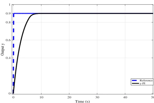
First, the effectiveness of the PI-AW controller would be checked without the pres-ence of Gaussian noise in the feedback loop, i.e., standard (σ₌0.0).

Figure 11 – System response without noise

0 10 20 30 40 50

Time (s) 0

0.4 0.6 0.8 0.9 1

Output y

Reference y-PI

(29)

Figure 12 – Control signal given to the plant

0 10 20 30 40 50

Time (s) -1

-0.8 -0.6 -0.4 -0.2 0 0.2 0.4 0.6 0.8 1

Control û

û-PI

U

max

U

min

Source: Author

From Figures 11 and 12 show that the controller responds properly obtaining a steady state error equal to zero, but the control signal to stay near the upper limit.

(30)

Figure 13 – System response with noise.

0 10 20 30 40 50

Time (s)

0 0.4 0.6 0.8 0.9 1

Output y

Reference y-PI

Source: Author

Figure 14 – control signal given to the plant.

0 10 20 30 40 50

Time (s) -1

-0.8 -0.6 -0.4 -0.2 0 0.2 0.4 0.6 0.8 1

Control û

û-PI

U

max

U

min

Source: Author

Steady-state error present in the system response (see Figure 13) depends on the Gaussian noise measurement power and this depends of the standard deviation σ. Therefore,

(31)

3 CONTROLLERS DESIGNS

In this chapter will be performed the theoretical foundation of the controllers ad-dressed in the present work: Firstly place, it is explained the strategy of the classical PI con-troller and its respective Anti-windup structure, i.e., PI-AW and the parameters tuning. Secondly place, for MPC controller, it will be made a brief introduction of its evolution, up until the GPC control. It should be noted that there will be two forms of optimization as numerical and ana-lytically, which is used in the present work. Finally, will review the concepts of performance indices TV, IAE, which will help us to relate a comparison between the controllers described in this chapter.

3.1 Proportional Integral Control

The PID is a controller that have techniques consolidated projects that determine the values of gains proportional, integral and derivative based on the final characteristics desired of the closed loop system as time of settlement and overshoot (OGATA, 1997).

The subsection will be studying the Anti-Windup technique for the PI controller, besides explaining the cause of the Windup phenomenon for this controller.

3.1.1 PI Control Structure

The structure of PI controller is showed in Figure 15:

Figure 15 – Structure of the PI controller.

e

u

Σ

R

(

z

)

Y

(

z

)

P

(

z

)

K

_p

K

i _z₋z₁

Source: Author.

(32)

The PI control is given by the following Equation (3.1) in the frequency domain.

CPI(s) =Kp+ Ki

s , (3.1)

or in discrete-time equivalent is:

CPI(z) =Kp+ Kiz

(z₋1). (3.2)

Then the equation of output of the PI controller in the time is:

u(t) =Kpe(t) +Ki

Z t

0 e(t)dt, (3.3)

or in discrete-time equivalent is:

u(z) =Kpe(z) +Ki z

z₋1e(z), (3.4)

whereR(z)is set-point of the system at timet, e(z)is error of the system at timet, Y(z)is result of output of the plant at timet. So controller is based on two parameters which are:

• Proportional Gain ConstantKp:

In proportional control, the actuating signal for the control action in control system is propor-tional to the error signal. The error signal is being the difference between the reference input signal and the feedback signal obtained from the output. For satisfactory performance of a control system, a convenient adjustment has to be made between the maximum overshoot and steady state error. Through the help of proportional constant without sacrificing the steady state accuracy, the maximum overshoot can be reduced to same of actuating signal.

Figure 16 – Proportional control action.

Source: Author.

(33)

For integral control action, the actuating signal consists of proportional-error signal added with integral of the error signal. By the help of an integrator is reduces the steady state errors through low frequency compensation. So the integral term will do the actual variable will track the reference more quickly. Ki=1/Tirepresents the integrative time.

Figure 17 – Integral control action.

Source: Author.

3.1.2 Controller adjustment methods

In the theory of control, there are different tuning methods for the parameters of the PI or PID control being used (ZIEGLER; NICHOLS, 1942; COHEN; COON, 1983; LOPEZet al., 1976). Therefore, it will cite the method used in the present work.

3.1.2.1 Root Locus Method

The study Root Locus has demonstrated for years one of the most useful tools in the synthesis of controllers. Then the design of a controller consists of placing the poles and zeros of the transfer function of the system in closed loop, in the most convenient positions in order to achieve a response according to certain specifications, generally in the time domain. then is described is the method through the following steps (RAMAKRISHNAN, 2017):

a) This defines the graph in thezplane of all the poles and zeros of the closed-loop transfer function.

1+Cc(z)P(z) =0 (3.5)

where Cc(z) is the regulator implemented in the digital controller and P(z) is the

transfer function of the plant in the z-plane. b) Module Condition

(34)

c) Condition of Angle or Phase

Ang(Cc(z)P(z)) = (2n+1)πrad. (3.7)

As shown in section 4.3.2 through the process of speed loop identification, the sys-tem can be satisfactorily represented for a model of first order with integrator:

Gpv= Kpv

z₋1. (3.8)

The PI discrete controller is represented by Equation( 3.9).

Gc(z) =

Kc(z−zc)

(z₋1) , (3.9)

whereKc andzc represent controller gain and controller zero position respectively. The

open-loop functionLc(z)of the system will be:

Lv(z) =

KcKpv(z−zc)

(z₋1)2 =

K1(z₋zc)

(z₋1)2 , (3.10)

beingK₁=KcKpv.

The transfer function closed-loop have two real poles and identical zp there is a

controller with a fast response and without overemphasis. The equation characteristic of system is expressed in Equation (3.11).

z2+ (K1−2)z+ (1−K1zc) =0. (3.11)

Thus, solving Equation (3.11) through the Bhaskara formula and comparing with the equating

zp it observes that the gain of the open loopK1is related to the poles position by the following

Equation (3.12).

K1=2−2zp. (3.12)

Through the discriminant of Equation (3.11) and using Equation(3.12) it obtains the expression that determines the zero position of controller:

zc=− K₁₋4

4 . (3.13)

(35)

3.1.3 Anti-Windup PI

Next is reviewed the popularTechnique Tracking Mode, the structure of this method is shown in Figure 18 (ASTRöM; HäGGLUND, 1995).

Figure 18 – Structure of PI-AW controller technique Tracking Mode.

u

û

Actuator

e Umax

Umin

Σ

Σ Σ

Σ

R(z) Y(z)

P(z) Kp

Ki

Kaw

z z−1

eaw

Source: (ASTRöM; HäGGLUND, 1995)

The inclusion of the saturator in control signal is related to the operating limits of the actuators (SHIN; PARK, 2012; SAKAI; ISHIDA, 2016) and it is given by Equation (2.1).

Where the new equation after the saturator (see Equation (2.1)) applied to the plant with Anti-windup is given by:

u(z) =Kpe(z) +Ki z

z₋1[e(z) +Kaw(ˆu(z)−u(z))] (3.14) The notion of proportional band is useful to understand the Windup effect. The proportional band is defined as the range of process outputs where the controller output is in the linear range. For a PI controller it has (ASTRöM; HäGGLUND, 1995):

ymax =ysp+

I₋Umax

K (3.15)

ymin=ysp+

I₋Umin

K (3.16)

The controller operates in the linear mode, if the predicted output is in the propor-tional band (Denotes the maximum control error the controller can handle with the available control signal). The control signal saturates when the predicted output is outside the propor-tional band. Notice that the proporpropor-tional band can be shifted by changing the integral term.

(36)

inside the linear limit of the actuator. In Figure 18, the system presents an additional feedback-loop. The difference between input and output of the actuator constitutes an error eaw that is

added to the input of integrator with a gain of (Kaw=1/Taw). When the saturation does not

exist, the erroreawis null and the controller is operating in the linear region. In other words, the

signaluis not saturated. If there is saturation,eawis different from zero. The time taken by the

integrator input to tend to zero is determined by the gain 1/Taw, whereTawcan be interpreted as

the time constant that determines how fast the input of the integrator becomes zero. The selec-tion of small values forTawcan be advantageous. However, a small value choice forTawshould

be carefully made, especially for systems with derivative action. What may happen is that the measurement noise can take the output of the controller into saturation state, resulting in a fast actuation of the anti-windup loop and making the input of the controller undesirably zero. In practice, an empiric selection of rule suggestsTaw=√TiorTaw=Ti(ASTRöM; HäGGLUND,

1995; HU; LIN, 2001b).

3.2 Model Predictive Control

Model predictive control (MPC) has been a control strategy widely used and investi-gated in both industry (in applications in the process, chemical, food processing and paper indus-tries) and academia. The main reason of this control strategy came by his great capacity of work with all kinds of processes and primarily by handling processes constraints implicitly. For the majority of cases, the optimization problem formulated in MPC is given for a single objective problem. Some of the most popular MPC algorithms well accepted in industry are the Dynamic Matrix Control (DMC) (CAMACHO; BORDONS, 1999), Model Algorithmic Control (MAC) (ALLGöWER; ZHENG, 2000), Predictive Functional Control (PFC) (ALLGöWER; ZHENG, 2000), Extended Prediction Self Adaptive Control (EPSAC), Extended Horizon Adaptive Con-trol (EHAC) and Generalized Predictive ConCon-trol (GPC) (CAMACHO; BORDONS, 1999). In this work, among these number of MPC algorithms, GPC is particularly studied to its impor-tance and popularity.

3.2.1 GPC Controller

(37)

im-plemented in many industrial applications, showing good performance and robustness. The ba-sic idea of GPC is to compute a sequence of future control signals in such a way that it minimizes a multistage cost function defined over a prediction horizon, given by (CAMACHO; BORDONS, 1999):

J₍_N₁_,_N₂_,_N_u₎=

N2

∑

j=N₁

δ(j)[y(t+j_|t)₋w(t+j)]2+

Nu−1

∑

j=0

λ(j)[∆u(t+j₋1)]2. (3.17)

whereN1andN2 are the prediction horizons minimum and maximum respectively,

Nuis the control horizon, λ andδ are positive weighting matrices,w(t+j)is the future

refer-ence trajectory,∆uis the incremental control action∆=1₋q−1, withq−1represents the delay operator, u(t+j₋1)is the incremental control and y(t+ j_|t) is the prediction of output y(t) from the instantt.

The GPC algorithm is based on ControlledAuto Regressive Integrated Moving

Aver-age(CARIMA) model and can be described after linearization considering the operation around a particular set point of a SISO (Single Input, Single Output) plant, then can be described as (CAMACHO; BORDONS, 1999):

A(q−1)y(t) =q−dB(q−1)u(t₋1) +T(q−1)e(t)

∆ , (3.18)

whereA(q−1),B(q−1),T(q−1)are polynomials in the form of delay given byq−1:

A(q−1) =1+a1q−1+a2q−2+···+anaq−

na_, (3.19)

B(q−1) =b0+b1q−1+b2q−2+···+bnbq

−nb_, (3.20)

T(q−1) =1+t₁q−1+t₂q−2+_···+tnTq−

nT_, (3.21)

where y(t) is the output of the system at instantt, u(t) is the input of system at instantt, ∆

is the integration operator given by ∆=1₋q−1, q−d describes the natural delay, in multi-ples of the sampling period, e(t) is a white noise of zero mean and variance σ2, the indices na, nb and nT are the degrees of the polynomials A(q−1), B(q−1) and T(q−1) respectively

(CAMACHO; BORDONS, 1999; MEGíASet al., 1997).

The last term of the Equation ( 3.18) can be written as:

n(t+j) = T(q− 1₎

(38)

where T(q−1) is a polynomial, ∆ is (1₋q−1) and e(t) is the prediction error. A necessary condition is that the degree of polynomialsT(q−1)andA(q−1), complynT ≤na+1.

Second (MCINTOSH S. L. SHAH, 1991) and (LAMBERT, 1987), the polynomial

T(q−1) is of second order, which sufficient for to constitute a low pass filter. Thus by the characteristics of study plants in this thesis was chosen the T-polynomial as:

T(q−1) = 1₋αq−1 1₋αq−1. (3.23)

The tuning variable for disturbance and noise rejection depends of poleα, which to stay between 0_≤α _≤1, because the cutoff frequency isFc=−ln(

α)

Ts (BORDIGNON, 2016).

The calculation of predictions is recursively performed from theDiophantine equa-tion, then the Equation (3.18) turns to:

∆A(q−1)y(t) =q−dB(q−1)∆u(t₋1) +T(q−1)e(t). (3.24)

In order to perform output predictions j₋steps ahead, one must write the above Equation (3.24) as follows:

∼

A(q−1)y(t+j) =B(q−1)∆u(t+j₋1) +T(q−1)e(t+j), (3.25)

where∆A=∼A(q−1)whose grade isna+1, then: ∼

A(q−1) =1+a˜₁q−1+a˜₂q−2+_···+a˜na+1q−

(na+1)_, (3.26)

The term related to the noise in Equation (3.25) is then decomposed by applying Diophantine Equation (3.27) leading to:

T(q−1) ˜

A(q−1) =Ej(q

−1_{) +}q−jFj(q−1)

˜

A(q−1) . (3.27)

Which may be rearranged as:

T(q−1) =∼A(q−1)Ej(q−1) +q−jFj(q−1); (3.28) Ej(q−1)A˜(q−1) =T(q−1)−q−jFj(q−1). (3.29)

where Ej(q−1) and Fj(q−1) are uniquely defined polynomials whose degrees are (j−1) and

(39)

T(q−1)by∼A(q−1), until the rest of the division can be factorized asq−jFj(q−1). The quotient

of the division is the polynomial Ej(q−1). If both members of Equation (3.25) are multiplied

byEj(q−1).

Ej(q−1)∆A(q−1)y(t+j) =Ej(q−1)B(q−1)∆u(t+j−1) +Ej(q−1)T(q−1)e(t+j), (3.30)

Substituting in Equation (3.29) as:

[T(q−1)₋q−jFj(q−1)] ∼

Ay(t+j) =Ej(q−1)B(q−1)∆u(t+j−1) +Ej(q−1)T(q−1)e(t+j), T(q−1)y(t+j)₋q−jy(t+ j)Fj(q−1) =Ej(q−1)B(q−1)∆u(t+j−1) +Ej(q−1)T(q−1)e(t+j), T(q−1)y(t+j)₋y(t)Fj(q−1) =Ej(q−1)B(q−1)∆u(t+j−1) +Ej(q−1)T(q−1)e(t+j),

y(t+j) = Fj(q

−1₎ T(q−1)y(t) +

Ej(q−1)B(q−1)

T(q−1) ∆u(t+j−1) +Ej(q

−1₎_e₍_t₊_j₎_, (3.31)

Since the degree of Ej(q−1) equal (j−1), then all the terms of the noise are in the future,

therefore the optimal prediction is obtained by changing e(t+j) by its expected value (zero), thus:

y(t+j_|t) = Fj(q− 1₎ T(q−1)y(t) +

Ej(q−1)B(q−1)

T(q−1) ∆u(t+j−1), (3.32) From Equation ( 3.32) the past control inputs can be separated from the present and future control by solving a new Diophantine equation as:

Ej(q−1)B(q−1)

T(q−1) =Hj(q

−1_{) +}_q−j_M₍_q−1₎_. _(3.33)

which can be written as:

Ej(q−1)B(z−1) =Hj(z−1)T(q−1) +q−jT(q−1)M(q−1), (3.34)

Ij(q−1) =T(q−1)M(q−1), (3.35)

Ej(q−1)B(q−1) =Hj(q−1)T(q−1) +q−jIj(q−1), (3.36)

whereHj with degree of j−1 and it is a matrix of response to the unit step ofP(q−1). Using

Equations (3.36) and (3.33) the output predictions can be rewritten as:

y(t+j_|t) =Hj(q−1)∆u(t−1+j|t) +Fj(q−1) y(t) T(q−1)+

Ij(q−1)

(40)

Since the point of view the controller implementation , an analytical solution with low computational cost is important since the implementation will be carried out in the DSP. Thus in this sense, this work addresses the special case where Nu=1, N1=0, N2 =N and

λ ₌0. Interactively solving Equation (3.37) is obtained:

y(t+1_|t) =H₁(q−1)∆u(t₋1+1_|t) +F₁(q−1) y(t) T(q−1)+

I1(q−1)

T(q−1)∆u(t−1), y(t+2_|t) =H2(q−1)∆u(t₋1+2_|t) +F2(q−1) y(t)

T(q−1)+

I2(q−1)

T(q−1)∆u(t−1), ...

y(t+N_|t) =HN(q−1)∆u(t−1+N|t) +FN(q−1) y(t) T(q−1)+

IN(q−1)

T(q−1)∆u(t−1),

(3.38)

Can be written in vectorial form:

y=G∆u+F(q−1) y(t)

T(q−1)+I(q

−1₎∆u(t−1)

T(q−1) , (3.39)

where the variablesy(t)and∆u(t₋1)are filtered byT(q−1)(CAMACHO; BORDONS, 1999). Gis a matrix based on the coefficients ofHj(q−1), of the form:

G= [h₁ h₂ _··· hN]Tr, (3.40)

Tr is transposed of the vector or matrix.

f=F(q−1) y(t)

T(q−1)+I(q

−1₎∆u(t−1)

T(q−1) , (3.41)

fis the free response, so:

y=f+G∆u (3.42)

Therefore, the Equation ( 3.17) can be written as:

J= (G∆u+f₋w)Tr(G∆u+f₋w) +λ∆uTr∆u, (3.43)

developing Equation ( 3.43) as:

J= (G∆u)TrG∆u+ (G∆u)Tr(f₋w) + (f₋w)TrG∆u+ (f₋w)Tr(f₋w) +λ∆uTr∆u,

J= [(G∆u)TrG+ (f₋w)TrG+λ∆uTr]∆u+ (G∆u)Tr(f₋w) + (f₋w)Tr(f₋w),

J= [∆uTrGTrG+ (f₋w)TrG+λ∆uTr]∆u+∆uTrGTr(f₋w) + (f₋w)Tr(f₋w),

J=∆uTr(GTrG+λI)∆u+2(f₋w)TrG∆u+ (f₋w)Tr(f₋w).

(41)

The parameters are:

H=2(GTrG+λI), (3.45)

bTr₌_2(f

−w)Tr_G

, (3.46)

f0= (f−w)Tr(f−w). (3.47)

Thus it obtains the following cost function to minimize of Equation ( 3.44) as:

J= 1 2∆u

Tr_H_∆_u₊_bTr_∆_u₊_f

0, (3.48)

The solution to this problem optimization is a crucial step in the algorithms based on GPC. Numerical complexity depends on the model characteristics in terms of linearity, con-straints, number of controlled and manipulated variables, etc., and then it has two cases:

3.2.1.1 Unconstrained optimization

In a non-restricted case ,i.e., without saturation the controller which minimizes the cost function according to Camacho (CAMACHO; BORDONS, 1999) is analytically calculated as:

Note:It is known that the gradient of a function of type: ∂_∂g_x= (A+ATr_)x₊_b_.

∂J ∂u =

1

2 H−H

Tr

∆u+b. (3.49)

AsHis symmetric , therefore:

∆u=₋H−1b. (3.50)

When it is used a sliding horizon strategy, the control signal applied to process is represented for the first element of second vector is given by:

∆u= (GTrG+λI)−1GTr(w₋f). (3.51)

As in practice only the current control action is applied, it has:

(42)

where K is equal to the first line of (GTr_G₊_λ_I)−1_GTr _{with dimension 1x}_N_, _G _is _N_x_N u

constant matrix based on the coefficients Hj(q−1) and w is a vector of the future reference

(SIMKOFFet al., 2017).

The controller implementation standpoint, an analytical solution with low computa-tional cost is important. Thus, this work is concerned a N=Nu=1, and λ =0, which

repre-sents the best trade off between computational cost and closed-loop performance (SILVAet al., 2013).

For the application it is proceeded to synthesize this digital controller in the structure known as RST, which allows the study of aspects related stability and robustness for linear controllers. Then the equation of a digital controller in theRSTform is:

u(t) = 1

∆R(q−1)

_T(

q−1)r(t)₋S(q−1)y(t)

, (3.53)

of the Equation (3.52):

∆u=

N

∑

i=1

Ki[w(t)−f(t)]. (3.54)

Substituting the free answer for its equivalence given by Equation (3.41), it has that:

∆u=

N

∑

i=1

Kiw(t)− N

∑

i=1 KiFi

y(t) T(q−1)−

N

∑

i=1 KiIi

∆u(t₋1)

T(q−1) , (3.55)

"

T(q−1) +q−1 N

∑

i=1 KiIi

#

∆u(t) =T(q−1)

N

∑

i=1

Kiw(t)− N

∑

i=1

KiFiy(t), (3.56)

u(t) = 1

∆

T(q−1) +q−1∑N_i₌₁KiIi

"

T(q−1)

N

∑

i=1

Kiw(t)− N

∑

i=1

KiFiy(t)

#

. (3.57)

Through some manipulations, Equation (3.53) can be written in theRSTform (ALMEIDAet al., 2014):

r(t) =w(t+i), (3.58)

is the setpoint and:

T(q−1) =T(q−1)

N

∑

i=1

Ki, (3.59)

S(q−1) =

N

∑

i=1

(43)

R(q−1) =T(q−1) +q−1 N

∑

i=1

KiIi(q−1). (3.61)

The controller proposed by (ALMEIDAet al., 2014) is designed to filter the control signal. Be-sides a tuning the controller is based on a single parameterα that allows good trade-offs among

noise attenuation of the control signal, disturbance rejection and system robustness during oper-ation, called GPC based control (GPCBC). Thus, the control polynomialsR,S, andTare given by (DIAS, 2016):

T(q−1) = (1−α)T(q− 1₎

b0 , (3.62)

R(q−1) =1₋αt₂q−1, (3.63)

S(q−1) = 2−α+t1+αt2−(1+αt1+ (2α−1)t2)q− 1

b0 , (3.64)

α =1₋ 1+2+3+···+N

1+22₊₃2₊_···₊_N2. (3.65)

It is observed that the polynomials R, S, T, contain the alpha parameter which depends on N. From Equation (3.65) it is readily seen that α =0 if N =0 and α _→1 as N _→∞. Therefore, for this approach prediction horizonN may be used as a setting parameter (DIASet al., 2016). From hereafter it is appliedα as an adjustment parameter in this work.

Figure 19 – Classical RST structure applied to SRM speed control. Actuator

SRM R

T 1 _ZOH

Gaussian Noise mean=0 S

Umax

Umin

ω_{re f}_. ω_ouput

Standard deviation=σ

Σ Σ

Source: Author.

The analysis of this diagram lead to the following transfer functions relating refer-enceω_{re f}_.=R(z)with outputω_ouput =Y(z), alongside with input disturbanceM(z), and output Gaussian noiseN(z), by the equations:

HY−R(z) = Y(z) R(z) =

T(z)G(z)

(44)

HY−M(z) = Y(z) M(z) =

∆R₍z)G(z)

∆R(z) +S(z)G(z), (3.67)

Hu−n(z) = u(z) n(z)=

−S(z)

∆R(z) +S(z)G(z), (3.68)

HY−N(z) = Y(z) N(z) =

−S(z)G(z)

∆R(z) +S(z)G(z). (3.69)

3.2.1.2 Constrained optimization

The main advantages of the GPC predictive control is its ability to incorporate con-straints in the design of the controller (BANERJEEet al., 2017), by taking numerical optimiza-tion, instead of analytical one described in the previous section.

Constraints may be related to limitations on the maximum and minimum magni-tudes of the control action described by:

Umin≤u(t+j|t)≤Umax , ∀j=0, . . . ,Nu−1, (3.70)

In addition, one may consider limitations on the speed of variation of control action:

∆umin≤∆u(t+j|t)≤∆umax , ∀j=0, . . . ,Nu−1, (3.71)

And also limitations on the maximum and minimum quantities allowed for the out-puts:

ymin≤y(t+j|t)≤ymax , ∀j=1, . . . ,N2, (3.72)

In this work the only restriction to be a consideration is the saturation for the control signal that relates a real process with restrictions (HUANGet al., 2017).

Thus now is form a matrix as:

1(Umin−u(t−j))≤Qu≤1Umax−u(t−j) ,∀t, (3.73)

where 1 is a unitary matrix Nux1 and Q is a lower triangular matrix NuxNu with unitary

(45)

interval[t,t+Nu−1], the restriction given by Equation (3.73) is satisfied if it is used in solving

the optimization problem. Rewriting Equation (3.70) in a more compact form.

Pu_≤c, (3.74)

where:

P=





Q

−Q



;c= 



1(Umin−u(t−1)) −1Umax−u(t₋1)



. (3.75)

Therefore, the optimization problem to be solved, is given as:

Minimize: J= 1

2∆u

Tr_H_∆_u₊_bTr_∆_u₊_f

0, (3.76)

sub ject to:Pu_≤c. (3.77)

The literature presents several numerical methods to solve the optimization problem with some described in (CAMACHO; BORDONS, 1999). A disadvantage in solving the opti-mization problem is the computational effort involved, which may require time not available in certain practical cases.

The problem of cost function optimization J with linear constraints (saturator) is usually known as a Quadratic Programming (QP) problem (HUANGet al., 2017). Such solu-tion is based on convex analysis (minimizasolu-tion problem) of the control signaluon a convex set, resolved numerically (CAMACHO; BORDONS, 1999). MATLAB command quadprog is a well known and efficient implementation to solve Equation (3.76).

u=quad prog(H;b;P;c) (3.78)

Figure 20, future reference (Ref) is subtracted from the future predicted outputs by the model (Ym). This difference of error (e) is introduced in the optimizer, that calculates an optimal output (u) (taking into account the cost function), also considering the restriction of the saturation (Umax,Umin) and then it is introduced into the process (Plant). After the process

(46)

Figure 20 – GPC-T controller with constrained

e D/A Plant

A/D Model Plant Optimizer Cost Function Future errors Future Inputs Future Reference Future Predicted Ouputs Constraints Ouput GPC-T Umax Umin Gaussian Noise mean=0 Umax Umin

Standard deviation=σ

Source: Author.

3.3 Performance Indices

To evaluate the dynamic behavior of the control systems and to compare the good-ness of the tuning methods studied in this work, it has been chosen the following performance indices (DORF; BISHOP, 2011):

− Integrated Absolute Error (IAE)

The IAE provides the area under the error curve, which represents the amount of material out of specification, energy lost or other undesired characteristic. TheIAE is given by the following equation:

IAE =

Z ∞

0 |e(t)|dt, (3.79)

wheree(t) =r(t)₋y(t), r(t)is the process reference and y(t) and is the output of process. If IAE _→0, theny(t)_→r(t)_∀t if the control were perfect.

Although the magnitude of the IAE is an indication of the goodness of the tuning method with respect to error is more useful, for comparison effects with respect to other tuning methods, its relative value with respect to the value of the IAE that would be obtained if the parameters of the controller were optimal with regard to that criterion (OGATA, 1997).

− Total Variation (TV)

the Integral of absolute values of the error TV is also a performance criterion for closed-loop response, but in contrast to theIAE, the objective forTV is to measure the total variation in the controller output signal,u.

TV = Z ∞ 0

(47)

or

TV =

∞

∑

i=0|

ui+1−ui| (3.81)

whereuiandui+1are the signal of present and future control, respectively (ROJAS, 2011). The desired valueTV, as well asIAE is to have low values.

− Steady State Error (ess)

The steady-state error is that error that remains after of what finish the transient. In which the signals of the system remain constant, while not having an external signal. This error can be calculated by the final value theorem, the limit of a function in the time domain, when time tends to infinity can be found through the product limit of the Laplace transform of the function by the Laplace variable, when it tends to zero (OGATA, 1997) .

ess(t) = lim

t→∞e(t)⇒ess=_slim_→₀sE(s) %ess=e¯ss∗100 (3.82) The desired value %ess is zero as ideal, but it is acceptable if it has a value close to zero that to

(48)

4 CASE STUDIES

This chapter is divided in two parts, the first one is intended to present compara-tive analysis for PI-AW and GPC-T controllers in different processes as stable and integracompara-tive plants. These plants are considered to be subjected to saturation in control signal and Gaus-sian noise in the feedback loop, in order to highlight the presence of the NITE phenomenon. In the GPC-T control with structure of the subsection 3.2.1.2 (see Figure 20) , the change parameter α of the T-polynomial do not has a relation direct with noise power is commonly

considered as a design parameter. Therefore, for this study α varies according to the values

α = [0,0,24,0,44,0,64,0,84,0,94], whose step is for a better appreciation of its evolution with

respect to the noise and mitigation of the NITE phenomenon. Finally, validate the comparison with the help of performance indices among the controls studied.

For the second part, as already described, it was used the laboratory prototype in the speed control of an SRM, whose details of the best setup are explained in the proper section of this work. Thus will perform comparative study of SRM speed control between the PI-AW and GPC-T controllers, under the presence of saturation and noise. The NITE phenomenon is investigated for such experimental plant and its respective mitigation by implementing the T-polynomial for the GPC controller under the same range previously selected forα, therefore for

the GPC-T controller is applying the equivalent structureRST(see subsection 3.2.1.1). Finally, it also validate the comparison by computing performance indices between the controllers.

Figure 21 – Comparison structure of the PI-AW and GPC-T controllers

PI-AW

GPC-T

or

Controller

Process Umax

Umin

u û

Actuator

Gaussian Noise mean=0 Σ

Σ

R(z) Y(z)

σ

(49)

4.1 Stable process

The case analyzed is a stable open-loop first order process, so the chosen plant is (EUN; S., 2015):

P(s) = 1

3s+1. (4.1)

The setting of the controllers to be compared are:

Firstly, for the PI-AW controller design, it has been considered the parametersKp=

5.5,Ki=3.1,Kaw=1, which are obtained through Root Locus Method (see subsection 3.1.2.1)

followed by a fine-tuning based on the simulation of the closed loop.

The GPC controller has been tuned with Ts =0.1[s],λ =17.1,N=Nu=100, in

order to exhibit output response similar to the PI-AW in the linear region (without Gaussian noise account)

For both controllers, saturation limits are: Umax=1 and Umin =0 and Set-point = 0.9. For this analysis, firstly it has been considered a step-like disturbance at time t =20s, without Gaussian noise. Results are shown in Figure 22.

Figure 22 – System response with perturbation and without noise

0 5 10 15 20 25 30 35 40 45 50

Time (s) 0

0.2 0.4 0.6 0.8 1

Output y

Reference y PI-AW y GPC-T α=0.0 y GPC-T α=0.24 y GPC-T α=0.44 y GPC-T α=0.64 y GPC-T α=0.84

y GPC-T α=0.94

20 22 24 26 28 30 32

0.9 0.91 0.92 0.93 0.94 0.95

(50)

Figure 23 – Control signal ˆu after saturator

0 5 10 15 20 25 30 35 40 45 50

Time [s]

0 0.2 0.4 0.6 0.8 1

Control û

û PI-AW û GPC-T α=0.0

û GPC-T α=0.24

û GPC-T α=0.44

û GPC-T α=0.64

û GPC-T α=0.84

û GPC-T α=0.94

20 22 24 26 28 30

0.7 0.8 0.9

Source: Author.

It is observed from Figure 22 that both controllers obviously have the same response in the transient and settling time, but for the GPC-T control the rejection of the disturbance depends on the T-polynomial and the election of the pole (α). In other words, disturbance

rejection can be made faster or slower based on the choice ofα. Thus whenα is increasing it has slower rejection asα _→1.

From Figure 23 one might note that the control signal stabilizes near the saturation limit, prior to the application of the step disturbance. It is elaborated right away Table 1 of comparison through the performance indices without noise in the feedback loop of PI-AW and GPC-T controllers.

Table 1 – Performance indices without noise for stable plant

Controller α IAE TV

PI-AW − 2.0654 1.1000

GPC-T 0.0 2.0041 0.2973

GPC-T 0.24 2.0088 0.2998

GPC-T 0.44 2.0158 0.3051

GPC-T 0.64 2.0312 0.3114

GPC-T 0.84 2.0907 0.3129

GPC-T 0.94 2.3218 0.2886

Source: Author.

Table 1 shows the performance indices of the PI and GPC-T controllers without the presence of noise. Note that IAE is roughly the same for both controllers, whenα =0 (see rows 1 and 2 of Table 1). However, GPC-T control exhibit considerably lower control effort as

(51)

the integral action immersed in these controllers.

Next, Gaussian noise is introduced with noise power σ ₌0.1 (standard deviation)

in the feedback loop, whose output response is viewed in Figures 24 and 25.

Figure 24 – System response with Gaussian noise (σ ₌0.1)

0 5 10 15 20 25 30 35 40 45 50

Time [s] 0

0.4 0.6 0.8 0.9 1

Output y Reference

y PI-AW

y GPC-T α=0.0 y GPC-T α=0.24

y GPC-T α=0.44 y GPC-T α=0.64 y GPC-T α=0.84 y GPC-T α=0.94

(52)

0 5 10 15 20 25 30 35 40 45 50

-1 0 1

û PI-AW

0 5 10 15 20 25 30 35 40 45 50

-1 0 1

û GPC-T α=0.0

0 5 10 15 20 25 30 35 40 45 50

-1 0 1

û GPC-T α=0.24

0 5 10 15 20 25 30 35 40 45 50

-1 0 1

û GPC-T α=0.44

0 5 10 15 20 25 30 35 40 45 50

-1 0 1

û GPC-T α=0.64

0 5 10 15 20 25 30 35 40 45 50

-1 0 1

û GPC-T α=0.84

0 5 10 15 20 25 30 35 40 45 50

Time [s] -1

0 1

û GPC-T α=0.94

Source: Author.

From Figures 24 and 25 is show that the PI-AW controller cannot follow the ref-erence because of the saturation in control signal, i.e., the NITE phenomenon observed in the article by (EUN; S., 2015). On the other hand, GPC-T controller also has steady-state error with the presence of Gaussian noise in the feedback loop, ifα ₌0 (of T-polynomial), and even greater than that of the PI-AW controller. However, asα _→1, NITE phenomenon is mitigated as noise peaks become smaller falling in the linear region (see Figure 24). Such a result is com-pliant with the fact that T-polynomial acts as a low-pass filter immersed in the calculation of the controller effort. (MEGíASet al., 1997; CAMACHO; BORDONS, 1999).

(53)

Table 2 – Performance indices with noise for stable plant

Controller α IAE TV %ess

PI-AW − 5.7413 115.1141 8.1105

GPC-T 0.0 30.7941 588.8031 61.3032 GPC-T 0.24 20.6534 395.5189 39.1749 GPC-T 0.44 12.5704 238.2452 23.2925

GPC-T 0.64 5.7025 105.9928 8.0017

GPC-T 0.84 2.5615 32.8221 0.1247

GPC-T 0.94 2.4425 8.5627 0.1094

Source: Author.

It concludes from this analysis, that in the presence of noise (see Table 2), the GPC-T controller (α =0.0) has greater steady-state error, in relation to the PI-AW control, by which they have lower performance. By increasingα in GPC-T control untilα₌0.94, the steady-state

error becomes to stay smaller (see Figure 24). Thus, the NITE effect is considerably reduced and its performance is improved relative to the PI-AW.

4.2 Integral process

The analyzed case is a process with integral action so the chosen plant is (HU; LIN, 2001b):

P(s) = 180

s(s+14). (4.2)

Setting of the controllers to be compared are shows as follows. Firstly, for the PI-AW controller design, it has been considered Kp=0.35, Ki=0.5, KAW =3.4, Ts=0.1[s],

obtained with the application of the Root Locus Method (see subsection 3.1.2.1) along with a tuning based on the simulation of the linear controlled system (without saturation and without Gaussian noise).

The GPC controller has been set withTs=0.1[s],λ =5,N=Nu=150, in order to

(54)

Figure 26 – System response with perturbation and without noise

0 5 10 15 20 25 30 35 40 45 50

Time (s) 0 20 40 60 80 100 120 Output y y PI-AW y GPC-T α_=0.0

y GPC-T α=0.24

y GPC-T α_=0.44

y GPC-T α_=0.64

y GPC-T α=0.84

y GPC-T α_=0.94

20 21 22 23 24 25

85 90 95 100 Reference Source: Author.

0 5 10 15 20 25 30 35 40 45 50

Time (s) -1 0 1 2 3 4 5 Control û û PI-AW û GPC-T α=0.0

û GPC-T α=0.24

û GPC-T α=0.44

û GPC-T α=0.64

û GPC-T α=0.84

û GPC-T α=0.94

20 21 22 23 24

3.5 4 4.5

Source: Author.

It is observed from Figure 26 that both controllers have the same response transient. But of the GPC-T control disturbance rejection, already mentioned above, is based on the T-polynomial pole (α), to be fast or slow. So both controllers have a steady-state erroress=0. It

should be noted that the control signal stabilizes near the saturation limit without considering the disturbance.

(55)

Table 3 – Performance indices without noise for integral plant

Controller α IAE TV

PI-AW − 94.1187 10.1380

GPC-T 0.0 89.1394 10.9810

GPC-T 0.24 90.1831 10.6266

GPC-T 0.44 91.8975 10.5856

GPC-T 0.64 96.1499 10.5636

GPC-T 0.84 117.7992 10.2297

GPC-T 0.94 245.8966 9.7702

Source: Author.

From Table 3 it can be verified that these controllers have the same characteristics. Then its comparison is feasible and it arrives at the same analysis of the stable plant, in the influence of T-polynomial with respect to the speed of disturbance rejection.

Following, Gaussian noise is introduced in the feedback loop with standard devia-tion (σ ₌5), leading to output responses seen in Figure 28 and 29.

Figure 28 – System response with Gaussian noise (σ =5)

0 5 10 15 20 25 30 35 40 45 50

Time (s)

0 100 200 300 400 500 600

Output y

Reference y PI-AW y GPC-T α=0.0

y GPC-T α_=0.24

y GPC-T α=0.44

y GPC-T α_=0.64

y GPC-T α=0.84

y GPC-T α_=0.94