A Work Project, presented as part of the requirements for the Award of a Master Degree in Finance from the NOVA – School of Business and Economics
IFRS 9 – Expected Credit Losses Recognition:
Assessing the Effects of the New Expected Credit Losses Model on the Economy
PEDRO MIGUEL TIMÓTEO DE SOUSA MOUTINHO
3957
A Project carried out on the Master in Finance Program, under the supervision of: Filipa Castro
Abstract:
During disturbing financial times, the economy suffers from the lack of provisioning that companies exhibit. Under IFRS 9, regulators intend to mitigate this issue. The following research project provides evidence regarding the interactions between the Economic Cycle, Loans and Provisions plus the adverse effect of the latter on regulatory capital. Moreover, using an empirical approach, it updates existing literature regarding the influence provisions have on the upward and downward movements of the business cycles. Overall, the new standard may contribute to the stability of the economy but is dependent on its consistent and rigorous application by banks.
Keywords: Provisions; Financial Stability; Regulatory Capital; IFRS 9; Expected Credit
P a g e 3 | 35 (1) IAS and IFRS are the acronym for International Accounting Standard and International Financial Reporting Standard, respectively. IAS
standards were introduced between 1973 and 2001, while IFRS standards have been substituting the IAS since 2001.
Introduction
After the 2008 financial crisis, the International Accounting Standards Board (2014) and the Financial Accounting Standards Board (2016) have agreed to come up with a new standard that has the purpose of resolving what has been considered as the major weakness of financial accounting standards: the late recognition of credit losses. The newly created standard – IFRS 9 - focus on a more forward-looking methodology of accounting for financial instruments.
However, much concern has been recently expressed about the effects of the new accounting standards implemented in 2018. The change for financial institutions on moving from the IAS 39 to IFRS 9 (1), provides challenges both for themselves and for their stakeholders. Specifically, due to the new impairment model, instead of recognizing expected loan losses when they occur, entities will now have to forecast them, distributing provisions between periods of expansion and recessions (thus, steadier state levels) and having an impact on their capital requirements. Central banks, banking regulators, auditing and consulting firms are engaged on evaluating the impact, as the change can alter the economic cycle, lead to a misallocation of lending resources and possibly altering financial stability.
The main hypothesis to be tested in this paper is: The new accounting framework, IFRS 9, will contribute to the financial stability of the economy. Consequently, this research studies the new impairment model, providing evidence on the input that provisions and therefore, the new accounting basis, brings to the economy. This paper is structured as follows: Section 1 familiarizes the new impairment model and covers the literature review on the adoption and expected impact of IFRS 9. Section 2 details the methodology used over this paper and addresses the research questions, while section 3, 4 and 5 presents and examines the main results. Lastly, section 6 outlines the main outcomes, concluding remarks, limitations and suggestions for further research.
1. Literature Review
IFRS 9 is a new international financial reporting standard that has the mission of substituting IAS 39 and addresses the accounting of financial assets. The objective is to overcome some of the problems appointed to IAS 39, namely the late recognition of losses on lending and it divides into three major topics: 1. Classification and measurement of financial instruments; 2. Impairment (Expected Credit Losses (ECL) Model) and 3. Hedging.
Focusing on the second point for the development of this thesis and on held to maturity instruments, namely loans, when banks provide them to numerous people or entities, they are at the same time exposed to the borrower’s risk, that is, to the possibility of those entering in default. In those situations, and when the collateral is lower than the loan carrying amount, banks will face direct credit losses. With the new impairment model, banks are now required to set aside an amount (referred to as loss provisions) to cover for any expected losses on their lending. In terms of reporting adjustments to this account of loss provisions, an increase or decrease of the same is going to be reflected on the company’s income statement, recorded as a loss or gain, respectively. Now, the recognition of these provisions will occur with much more frequency as the new impairment model is grounded on the long-term, i.e. on a forward looking perspective, whereas IAS 39 only recognized incurred credit events, resulting in a backward-looking framework. Before, credit losses were only recognized if there was a clear sign of a credit event, being default situations or a delay to comply with loans obligations, prime examples of a credit event. Hence, the new impairment model is not expected to increase the amount of credit losses documented in a downturn. Rather, it will change how those same losses are distributed over time, recognizing a bigger portion of those in the beginning of a downturn, where expectations of defaults are starting to rise.
P a g e 5 | 35
(2) Expected Credit Losses (ECL) = Probability of Default (PD) * Loss Given Default (LGD) * Exposure at Default (EAD)
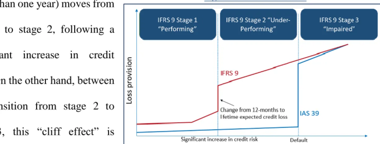
IFRS 9 divides the new impairment model into three layers, contingent on changes in credit risk since the beginning of the instrument’s life. In other words, banks should move their loans expected losses between stages if there is an increase or decrease in the expectation of those (Table 1). Therefore, interest revenue and expected credit losses (2) accounted in bank’s financial statements will vary as a function of the credit risk stage that financial assets are currently integrated in. Frykström, N. and Li, J. (2018) and Serrano, A.S. (2018), state that “a significant “cliff effect” in the provisions recognized could occur in those cases where the financial instruments (with maturity higher than one year) moves from
stage 1 to stage 2, following a significant increase in credit risk”. On the other hand, between the transition from stage 2 to stage 3, this “cliff effect” is
reduced when compared to IAS 39, under which is triggered by a default event (Figure 1).
Although the implementation of the new IFRS 9 is expected resolve the before mentioned concerns, it still has some challenges needed to be overcome. According to Leman, E (2015) it still is considered an open book since a lot of its components are assigned to the entities/regulators/accountant’s consideration (e.g. what a decrease in credit quality is). Also, since the expected loss model includes too much managerial discretion, the accounting of provisions may vary along different stakeholders. For example, with regards to timing, the moment when the transition between stages is triggered is subject to the judgment of the representatives and to their interpretation of the loan riskiness.
Table 1: Overview of the Impairment Model
Focusing on the effect that IFRS 9 can have on the financial stability of the economy, Laeven, L., Majnoni, G. (2003), Beatty, A. and Liao, S. (2011), and Bushman, R.M. and Williams, C.D. (2015) showed that by delaying the acknowledgment of expected credit losses, a negative response on financial stability will follow. The logic behind starts with macroeconomic variables, like unemployment, inflation or interest rates, that ultimately determine credit losses. When those start to deteriorate, payments are going to become due. However, between the first evidence of an economic downturn and the effective default, those delays in payments could be used by banks to anticipate the amount of credit losses, “enhancing their loss-absorbing capacity in downturns and ensuring a smooth provision of credit to the real economy afterwards” (Serrano, A.S. (2018)). Nevertheless, and quoting Novotny-Farkas, Z. (2016), “from a financial stability perspective, the concern is whether loan loss accounting amplifies the upward and downward swings of the business cycle”.
Additionally, Deloitte (2016) and Novotny-Farkas, Z. (2016) presented in their reports evidence regarding some of the consequences of IFRS 9. They consider that the measurement of loan loss provisions is strictly connected to capital requirements and will eventually have an impact in the economy as a whole, especially since banks are a key stakeholder for the economy (for example, the capital requirements will most likely affect the lending criteria, which can impact the sustainability and recovery of the economy). Also, the expected increase in provisions with the introduction of the new IFRS 9 will decrease retained earnings. As it is an important component of Common Equity Tier 1 (CET1) resources (Exhibit 1), the most loss-absorbent type of capital and that to which investors and regulators take most consideration, additional impairment will have an influence on capital resources.
Endorsing, Frykstrom, N. and Li, J. (2018) have estimated an increase between 13 and 25 per cent of provisions and a strong effect on banks’ capital requirements: “The total transitional effect of IFRS 9 on capital ratios is, mainly driven by the ECL requirements through increased
P a g e 7 | 35 provisions and the estimated transitional impact on CET1 ratio is a decrease around 45-50 bps” (Exhibit 2). Moreover, Beatty, A. and Liao, S. (2011), using a sample of U.S. banks, concluded that those that delay provisioning, will eventually reduce the amount of capital lent to the economy in comparison with banks that have smaller delays, due to insufficient capital resources and the subsequent difficulty to supplement capital in an economic downturn.
In other words, IFRS 9 is considered to have less pro-cyclicality when compared to IAS 39, particularly regarding to provisioning. According to Financial Stability Forum (FSF 2009), pro-cyclicality is considered as “the mutually reinforcing interactions through which the financial system can amplify business fluctuations and possibly cause or exacerbate financial instability”. Under the ECL approach, which indicates future macroeconomic conditions, the model specifies that credit losses should be accounted when the first indicators of economic distress begins to surface. This allows banks to recognise credit losses in an early stage which in turn are the periods where earnings are likely higher. Therefore, they will be able to prepare themselves to shoulder future losses (through the increase in capital reserves, given the level of provisions). That said, the new impairment model may contribute to the reduction of the downturns and upturns swings of the business cycle, thus enhancing economic stability (Exhibit 3). In periods where the economy is growing, the likelihood of a bank to recognise a provision under IAS 39 is almost zero. Thus, they will be overstating earnings and capital requirements over this period, allowing banks to increase their lending rate. On the other hand, in recessions, some unprovisioned loans will materialise and shrink CET1, followed by a decrease of the company’s profits. Furthermore, the cut in capital requirements and the risk associated to the current economic conditions will lead banks to either reduce loan growth or to raise new capital to comply with the capital standards applied. Nevertheless, due to financing frictions, it might be difficult for entities to issue equity. Having no other alternative, banks will decrease lending, which may result on a credit crunch. Overall, the new ECL model is expected to diminish some
of the features of IAS 39 that intensified pro-cyclicality as the “the recognition of 12-month ECL in Stage 1 in a sense serves as an adjustment to the credit spread that is recognised through the yield, and thus, results in less overstated profits” - Novotny-Farkas, Z. (2016).
Therefore, it is considered that the earlier accounting of expected losses and consequential provisions would smooth the up and downward movements of the business cycle. When using backward-looking, through economic expansions, there are fewer credit losses recognised, resulting in subordinate loss reserves. Alternatively, in recessions, loan loss provisions rise since defaults tend to increase over these stages. “As a result, the non-discretionary component is a driving force in the cyclicality of loan provisions and leads to a misevaluation” (Bouvatier, V. and Lepetit, L. (2006)). In addition, Keeton, W.R. (1999) and Jiménez, G. and Saurina, J. (2005) demonstrate that, typically, an increase of the lending rate in a thriving economic cycle is followed by an increase of credit impairments in slowdowns.
Nevertheless, according to Greenawalt, M.B. and Sinkey Jr., J.F. (1988) the income-smoothing hypothesis could mitigate provisioning effects. Management may seek to reduce the variability of their profits through accounting decisions. For example, banks may shift particular revenue or expenses to obtain yearly earnings with lower volatility. Therefore, the impact on financial stability by the IFRS 9 could be diminished. However, in his study, Scheiner, J. (1981) obtained results of smoothing behavior in only 21,5% of the sample used (107 large banks during 1969 to 1976). Thus, it was possible to conclude that "in general, banks do not appear to use the loan-loss provision as a device to smooth income".
2. Methodology
This research aims to infer how and to what extent can IFRS 9 back economic stability. Over this section, a description of the analysis conducted is described based on the research questions implemented as well as the samples and data used. The quantitative and qualitative analysis
P a g e 9 | 35 will focus on the level of provisions, which is considered to be the main variable associated with IFRS 9, and the impact it may have on financial stability.
In alignment with this project hypothesis, five research questions (RQ) were established:
RQ1: Do provisions tend to increase during economic expansions and decrease in downturns?
RQ2: Do provisions contribute to the decrease of capital requirements?
RQ3: Do loans granted by banks reduce after a decrease in CET1 ratio?
RQ4: Can provisions contribute to the financial stability of the economy?
RQ5: Will IFRS 9 ultimately have the same impact as provisions?
For the first research question, a simple quantitative analysis was used to conclude about the relationships between GDP, Provisions and Loans and how those are influenced. The data collected was obtained from 2 different sources: ECB and Pordata for European Union from 2007 to 2017.
Secondly, regarding research question 2 and 3, a sample of 10 major banks in the E.U. was used to obtain Tier 1 Capital and Retained Earnings (the two as a % of Assets) gathered from companies’ annual reports. Empirical data from literature was also gathered regarding the effect that capital requirements have on credit supply. These three research questions represent the deductive study of this paper and establishes the link between the increases in Provisions with pro-cyclicality. As discussed in the literature review, provisioning is influenced by the current and expected economic conditions, and its effects start on regulatory capital, moving on to the lending criteria before ending on the stability of the economy through pro-cyclicality.
Thirdly, for research question number 4 and to analyze the statistical influence that provisions have on economic financial stability, two types of regressions were performed: Panel data and Time-series. For the first one, the initial sample of the regression intended to include all the 28
countries of European Union plus United States for the period of 2008 to 2017. However, due to the lack of information available for some of these countries, the final sample ended up including only 23 European Union countries. Moreover, two time-series were also performed. One will feature E.U. and the other U.K. Both will represent a larger period of time, 1998-2017, bringing a different perspective into the analysis. However, since the total provisions of each country/region was only available from the beginning of 2007, a sample of the provisions from the 5 biggest banks in each region was gathered. For this research question the databases used were Pordata, ECB, World Bank, United Nations and OECD.
Lastly, and based on the answers to the previous research questions the results will be extrapolated to estimate the impact that IFRS 9 new impairment model has on the economy.
3. Deductive Study
3.1 Relationship between Provisions, Loan and GDP Growth (RQ1)
For the purpose of this paper it is important to better understand bank’s response to economic fluctuations and the relationship between Provisions and some macroeconomic conditions. Therefore, data was gathered through 2 different sources: World Bank and European Central Bank regarding European Union
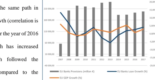
By analyzing figure 2, it is evident that Loan growth follows the same path in most years as GDP growth (correlation is equal to 0,52), except for the year of 2016 in which Loan growth has increased whereas GDP growth followed the opposite direction, compared to the
previous year – the first has increased 0,7 percentage points whereas the second has decreased
Figure 2: Provisions, Loans Issued and GDP Evolution in E.U.
-20,00% -15,00% -10,00% -5,00% 0,00% 5,00% 10,00% 15,00% 20,00% -40 000,00 10 000,00 60 000,00 110 000,00 160 000,00 210 000,00 2007 2008 2009 2010 2011 2012 2013 2014 2015 2016 2017
EU Banks Provisions (million €) EU Banks Loan Growth (%) EU GDP Growth (%)
P a g e 11 | 35 4,7 p.p. These results were the ones expected with both supply and demand as driving forces (during expansions, the lending rate plus the demand for loans is higher due to market confidence and opportunities). Indeed, the years where Loans had the biggest decrease were 2009, 2012 and 2013 (-1,77% ; -2,55% and -5,68%, respectively), periods where the macroeconomic conditions were struggling in the European Union, with Portugal and Greece as examples.
The relationship between Provisions and GDP growth, even though not obvious, looks like a negative one: when there is a reduction in the economy growth, usually the level of provisions tend to increase. Indeed, if a regression is performed with Provisions Growth as the dependent variable and GDP growth as independent one (Table 2), when GDP growth decreases by one percentage point, provisions increase by 10 percentage points, on average, ceteris paribus (correlation is -0,69). Truly, if there is an increase in the impaired loans due to economic instability (in other words, smaller or even negative growth rates of GDP) by accounting laws, banks needed to put aside provisions to cover for those impaired losses (IAS 39). Supporting, the most evidence scenarios of this concept occurred in the years of 2008, 2009, 2012 and 2013 which were the years where GDP growth was either negative or close to 0% and Provisions reached it biggest increase and highest historical values. Indeed, when Provisions registered the highest growth from 2007 to 2008 (261%), it was when GDP growth was almost zero - only 0,58%. These were the times where there were higher economy frictions, and consequently, a higher rate of defaults.
Lastly, the relationship between Provisions and Loan growth follows the same reasoning as GDP growth, i.e. there is a negative correlation between the two (-0,84), specifically in the
Table 2: Provisions Growth and GDP Growth Regression SUMMARY OUTPUT Regression Statistics Multiple R 0,24 R Square 0,06 Adjusted R Square -0,06 Standard Error 0,85 Observations 10 ANOVA df SS MS F Significance F Regression 1 0,37 0,37 0,50 0,50 Residual 8 5,85 0,73 Total 9 6,22
Coefficients Standard Error t Stat P-value Lower 95% Upper 95% Lower 95,0% Upper 95,0%
Intercept 0,43 0,36 1,20 0,26 -0,40 1,27 -0,40 1,27
period of 2007 to 2015. Therefore, we can infer that backward-looking provisioning amplifies the cyclicality of bank lending.
3.2 Impact of Provisions on Capital Requirements and Lending (RQ2 & RQ3)
Regardless of the accounting standards used, when there is a change in the level of provisions, it will affect banks income statement, their returns on equity and most likely their capital requirements. This happens because Provisions are considered as an expense and, hence are deductions from net interest income (a direct consequence of increasing provisions). When the level of dividends is fixed, a provisions increase will result in a decrease of retained earnings and, following the same reasoning, a decrease on banks regulatory capital (via its impact on Tier 1).
From a regulatory point of view, it is difficult to say whether an increase in provisions is desirable or not. By raising the level of provisions during economic expansions, the level of reserves applicable to absorb future expected losses might increase, while at the same time, depreciating the regulatory requirements buffers that entities have to mitigate other unexpected losses (e.g. sales reduction) (Exhibit 1). Nevertheless, it is also expected that if banks allocate these provisions during good times, they are limiting their capacity over this period, but in the long-run and in the possibility of a downturn, they are better prepared as the strike in capital requirements might not be so high due to the higher provision levels.
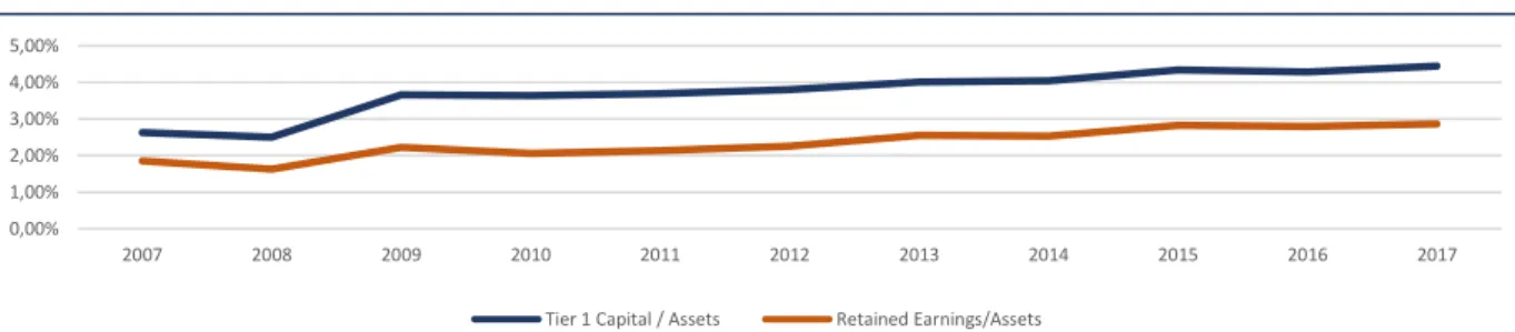
Even though the net effect of the offsetting rules is difficult to estimate, by observing historical evidence, one can get an idea of the extent to which provisioning can influence capital. It is important to highlight that we are considering that provisioning will only directly distress capital to the extent that it affects retained earnings. Figure 3 shows the retained earnings and tier 1 capital as a percentage of assets of Europe 10 major banks in 2018 (by total assets) from the period of 2007 to 2017.
P a g e 13 | 35
Figure 3: Tier 1 Capital, Retained Earnings and Provisions (% Assets) Evolution of Europe 10 major Banks
Table 3: Impact of one percentage point increase in capital requirements on credit supply Table 3: Impact of one percentage point increase in capital requirements on credit supply
Source: Martynova, N. (2015)
By observing Figure 3, it is possible to verify that there is a clear relationship between Tier 1 Capital and Retained Earnings over this period as expected (CET1 is composed mainly by common stock and Retained Earnings). So, if provisions have a direct and adverse impact on company’s profit, it will decrease banks’ capital requirements as expected.
Regarding the subsequent effects of capital requirements, when banks increase provisions they are reducing retained earnings. At the same time, an increase in provisioning is associated to riskier and fragile economic conditions (as discussed before in section 3.1), meaning that their risk weighted assets will increase. Consequently, when loan loss allowances increase, Core Tier 1 Capital ratio (𝐶𝐸𝑇1
𝑅𝑊𝐴) will reduce significantly (through the decrease of CET1 and the increase of RWA). Considering that Basel III requires banks to have at least 4,5% of core capital to total risk weighted assets (Exhibit 1), one of the few possible solutions is to cut lending supply. Doing so, banks will be reducing the risk associated to their total assets and CET1 decreases considerably less. Thus, capital ratios increase and comply with the capital requirements under Basel III. However, in recessions, this event results in shortage of credit supply and negatively impacts the economy, contributing, furthermore, to its depression. Additionally, according to most empirical evidence, it is possible to corroborate that in general, an increase in capital requirements will reduce total credit supply in the short-run between 1,2 and 4,6 percentage points, on average, ceteris paribus (Table 3)
0,00% 1,00% 2,00% 3,00% 4,00% 5,00% 2007 2008 2009 2010 2011 2012 2013 2014 2015 2016 2017
Tier 1 Capital / Assets Retained Earnings/Assets
Study Francis, W.B., and
Osborne, M. (2012) BIG MAG (2010)
Aiyar, S., Calomiris C. and
Wiedalek, T. (2014) Bridges et al. (2014) Mesonnier, J. and Monks, A. (2014) Noss, J and P. Toffano (2014)
Lending Reduction % 1,2 1,4 4,6 3,5 1,2 4,5
Sample Used U.K. 15 Countries U.K. U.K. France U.K.
Overall, with the new impairment model, although the impact of one percentage point increase of capital requirements on credit supply is expected to maintain the same, by spreading provisions between up and downturns, capital ratios volatility (in absolute terms) will be significantly reduced. Following the same rational, credit supply will also suffer less variations.
In conclusion, one can infer that the basis for the decrease of pro-cyclicality under IFRS 9 is established. According to section 3.1, banks usually react to economic struggles by increasing the level of provisions and, afterwards, reducing loans issuance. Moreover, as seen in section 3.2, provisioning will result in a decrease of bank’s capital requirements. Consequently, by spreading provisions over time and not only in impairment events, banks are strengthening their capital buffers for the future and their lending criteria will suffer lower reductions in worst economic periods. As capital supply is a key influencer on the amplification of the upwards and downwards swings of the economy, the level of provisions may contribute to the reduction of pro-cyclicality.
4. Econometric Study - Models and Data (RQ4)
Moving on to the most quantitative examination of this paper, the intent of the upcoming analysis is to confirm empirically whether the adoption of IFRS 9 can contribute to the reduction of pro-cyclicality, achieved through Provisions. Thus, further on, we will develop an econometric model (in this case a regression analysis). At first, the objective was to perform a time-series with a range of 30 years for the European Union, where the regressand is a variable that represents economic stability. For the independent ones, as the objective of study is the possible contribution of provisions, those are going to be included, plus other macroeconomic variables to control the true effect of loan loss allowances.
However, when accessing the various databases discussed in section 2, it was clear that gathering the data for 30 years for the European Union was unreasonable (data about provisions
P a g e 15 | 35
Figure 4: Dependent Variable
was only available since 2007). To face this challenge, two solutions arise: First, in order to overcome the small sample, a panel data was considered such that the amount of data available to perform the regression was wider and this way, increasing the robustness of the results. The data considers 23 countries across Europe over 10 periods (2008-2017). Secondly, the original idealized time-series will be performed, but in this case, only for the U.K. and the European Union where a sample of the 5 biggest banks is going to be considered to retrieve the data about provisions for the period of 1998-2017.
The identification of the variables used in the model will be presented with due justification: Dependent Variable:
Absolute value of GDP – GDP Trend: the variable reflects what is expected to be affected by the adoption of IFRS 9 – economic stability. By using this variable, we are obtaining the differences between the real GDP and the expected one based on previous years (using the trend function in excel). Doing so, we will be able to conclude on whether or not a variable can contribute to the reduction of the downturns and upturns swings of the business cycle and, thus, increasing the stability of the economy. The variable is in million euros (€) and the absolute value was used, since the objective is to conclude on the deviation of GDP from its trend, whether it is a positive or negative difference. Figure 4 pretends to better explain the variable in question, where the blue line represents the real GDP and the
black one, the trend.
Explanatory variables in study
Provisions: the relevant variable for the analysis of this paper represents the amount of provisions in the banking industry by country. This variable will help us understand the contribution of IFRS 9 to financial stability. The variable is in million euros (€) and we hypothesize a negative coefficient, since the expectation is that provisions will decrease the differences between GDP and its trend;
Control variables
Final Consumption: retrieved from World Bank, it is the total consumption made by private households plus the exchange of capital for goods and services. The currency used is in the current US dollar value ($), measured in millions, and we are expecting that higher consumption reduces financial instability, especially due to the potential of mitigating the downward movements of the economy through a fastest recovery,
offsetting the GDP increase in expansions (Keynesian Model);
Foreign Direct Investment (FDI): this variable was retrieved from World Bank and consists on an investment made by a company or individual in a different country than the one it is originally based in. The currency used is in million in the current US dollar value ($) and we are expecting that if FDI has an impact on financial stability, it will be a positive one; Net Exports: another World Bank data, which was calculated by making the difference
between a country’s exports and imports. Once again, we are expecting a negative relationship, i.e., a higher financial stability (using the same logic as Final Consumption and FDI), and it is measured in the current US dollar value ($) in millions;
Inflation and Inflation2: a World Bank indicator, represented in percentage that reflects the rate at which the prices for goods and services rise. This variable was also squared, since it was expected that it follows a polynomial function, where until a certain level, the higher the inflation, the higher is the expected financial stability of the economy but only until a certain point. For example, having a 1% of inflation is a good sign of financial stability but a -1% or a 3% will likely increase the volatility;
Unemployment: once again, a World Bank indicator that represents the total unemployed individuals divided in percentage of the labor force available. Evidently, we are expecting a negative correlation between unemployment and the measured variable;
P a g e 17 | 35 Population Density: the data regarding this variable was retrieved in the World Bank website
where it represents the number of people per square kilometer. The hopes of this variable is that higher values represent lower fluctuations in the economy, since it is more challenging for an economy to oscillate when the population is bigger (the macro conditions would have to be worse than those countries with less population);
Education Index: a United Nations Indicator that measures the population education level by using average years of schooling as well as expected years of schooling. It ranges from 0 to 1. Consequently, the higher the index, the stable is the economy expected to be;
Political Stability: a World Governance Indicators regarding the level of political stability, lack of violence or terrorism, among others. To do so, it measures the perception of the probability of political instability or the occurrence of violence/terrorism moved by political causes. The index ranges from -2,5, which indicates higher likelihood of instability, to 2,5, indicating a strong performance with lower political risk. Thus, it is expected that the economy is stable in nations with a higher political stability.
Public Debt and Public Debt2: data retrieved in the OECD database, denotes the amount of outstanding debt a country has issued over the years and is measured as a percentage of the GDP. This variable was also squared due to the trade-off theory, i.e., until a certain optimal point, debt is favorable as it is cheaper. But since that point, due to the distress costs associated, a higher amount of debt brings companies/countries to an instable situation. This theory was, therefore, added to the regression, by assuming that there is an interval of this variable, where a higher Public Debt converts into higher financial stability. Nevertheless, it is important to highlight that the preliminary results of the panel data regression showed that this relationship does not apply (both coefficients had the same sign). Consequently, for the time-series regressions we included both variables, whereas for panel data regression only the standard public debt was included.
To study the aforementioned relations, we computed the following regression on Stata:
|𝐺𝐷𝑃 − 𝐺𝐷𝑃 𝑇𝑟𝑒𝑛𝑑| = 𝛽0+ 𝛽1𝑝𝑟𝑜𝑣𝑖𝑠𝑖𝑜𝑛𝑠 + 𝛽2𝐹𝐷𝐼 + 𝛽3𝑖𝑛𝑓𝑙𝑎𝑡𝑖𝑜𝑛 + 𝛽4𝑖𝑛𝑓𝑙𝑎𝑡𝑖𝑜𝑛2+ 𝛽5𝑈𝑛𝑒𝑚𝑝𝑙𝑜𝑦𝑚𝑒𝑛𝑡 +
𝛽6𝑃𝑜𝑝. 𝐷𝑒𝑛𝑠𝑖𝑡𝑦 + 𝛽7𝐶𝑜𝑛𝑠𝑢𝑚𝑝𝑡𝑖𝑜𝑛 + 𝛽8𝑁𝑒𝑡𝐸𝑥𝑝𝑜𝑟𝑡𝑠 + 𝛽9𝐸𝑑𝑢𝑐𝑎𝑡𝑖𝑜𝑛𝐼𝑛𝑑𝑒𝑥 + 𝛽10𝑃𝑜𝑙𝑖𝑡𝑖𝑐𝑎𝑙𝐼𝑛𝑑𝑒𝑥 + 𝛽11𝑃𝑢𝑏𝑙𝑖𝑐𝐷𝑒𝑏𝑡 +
𝛽12𝑃𝑢𝑏𝑙𝑖𝑐𝐷𝑒𝑏𝑡2+ 𝑖. 𝐶𝑜𝑢𝑛𝑡𝑟𝑦 + 𝑖. 𝑌𝑒𝑎𝑟 + 𝜀𝑖
4.1 Model Results
First of all, prior to proceeding with the analysis of the regressions it is important to clarify whether they have indications of autocorrelation (when there is a correlation between the dependent variable and its lagged form, over different time periods) and/or evidence of heteroscedasticity (when the variable standard deviation is not constant over time) between the variables, and possibly correct for it.
Starting with autocorrelation, in the panel data regression, the Wooldridge test was performed in Stata to measure autocorrelation in Panel Data (Exhibit 6). When analyzing the results, one concludes that the null hypothesis is rejected for a 5% significance value (p-value is 0,025), meaning that there is evidence of auto-correlation in this regression. On the other hand, to analyze autocorrelation in the time-series regression, the simple Durbin Watson test was used. For the U.K. a DW value of 2,095 was obtained whereas for E.U. it is 2,54 (Exhibit 8 and 10). By observing the Durbin Watson table, and considering that there are 12 regressors excluding the intercept and 20 observations, the lower and upper limit (dL and dU) are respectively 0,2 and 3,234 for a 5% significance value. Since both test results are allocated inside the interval of the lower and upper values, the test is inconclusive.
Secondly, for the existence of heteroscedasticity, Breusch Pagan test in Stata was performed where the null hypothesis is H0: Constant Variance. Regarding Panel Data (Exhibit 6), we obtain a p-value of 0. Consequently, for any significance value, the null hypothesis is rejected, and there is evidence of heteroscedasticity in this regression. However, for both time-series, the p-value of the Breusch Pagan test for the U.K. and E.U. is 0,97 and 0,81 respectively (Exhibit 7
P a g e 19 | 35
Table 5: Panel Data Regression using Robust Standard Errors Table 6: U.K. Time-Series Regression
and 9). That said, for the time-series regressions and for any confidence level, we do not reject the null hypothesis of constant variance and there is compliance with the homoscedasticity assumption. In Wooldridge, J. M. (2002), he presents a way of correcting for both heteroscedasticity and autocorrelation using a simple method – clustering. Cluster is a technique used, which consists on partition the data in clusters and then perform an individual multiple regressions within each cluster. If done correctly, the different clusters will exhibit minimal correlation from one another. This technique was applied to the panel data regression using the correspondent command in Stata – Cluster (country). However, by observing the preliminary results (Table 4), it was observed that by using this technique, only provisions would be significant at a 90% confidence level, although the 𝑅2 is considerably high (75%). That said, and since the goal of this research is to focus on the sign of the coefficients and the contribution of the IFRS 9 to financial stability and its components, the standard errors are not the main motivation in this study. Nevertheless, robust standard errors will be used for panel data, and automatically be correcting for heteroscedasticity. Now that we have described the variables and address violations of assumptions in Multiple Linear Regressions, we will proceed to the analysis using the tables below.
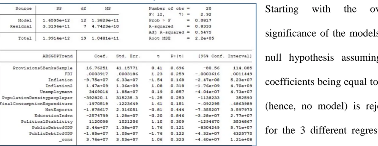
Table 7: E.U. Time-Series Regression
Starting with the overall significance of the models, the null hypothesis assuming all coefficients being equal to zero (hence, no model) is rejected for the 3 different regressions with a 10% significance value, with the smallest F-test being the time-series regression for the E.U - F(12;7) = 2,92 - while the panel data regression has the biggest one - F(42;187) = 13,83. Thus, we can state that all the models pass the overall significance test for a 10% confidence level.
Moving on to the overall fit of the models and significance level of the variables, although in the three regressions the variables used are the same, the time range and type of regression is different from the panel data regression to the time-series one. Therefore, the adjusted 𝑅2 (and not the normal 𝑅2) must be used to compare them and infer which the best one is, as the normal 𝑅2 assumes that all predictors have an impact on the deviation in the regressand, which may not be the case. The regression which has the higher adjusted 𝑅2 is the panel data (74%), meaning that the independent variables justifies 74% of the variation in the dependent one (3). Following, is the U.K. time-series regression with an adjusted 𝑅2 of 69% and then, E.U. with 55%. These results are encouraged since we are obtaining for the 3 different regressions, a big percentage in the adjusted 𝑅2. Nevertheless, the panel data is considered as the best regression to obtain the most reliable conclusions. Proceeding with the analysis, regarding the interpretation of the coefficients and their correspondent significance, we will perform the evaluation regression by regression.
Focusing on the one we consider as the best one – Panel Data – some variables are not significant at the 5% two-tailed significance value, namely FDI, Inflation, Inflation2,
P a g e 21 | 35
(4) The adjusted R2 was calculated based on the formula: 1 − (1 − 0,748) ∗ (230 − 1)/(230 − 7 − 1)
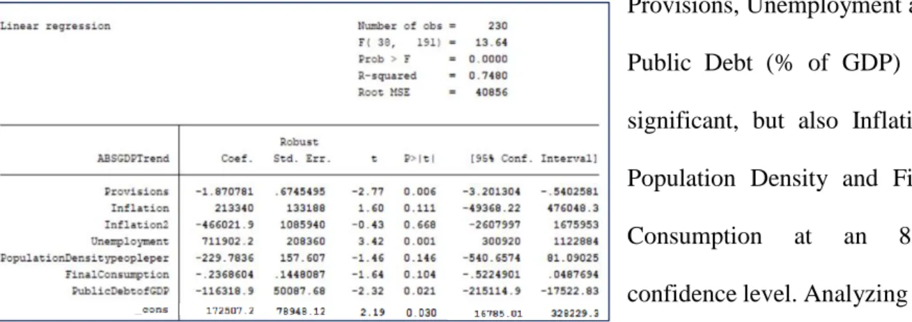
Population Density, Consumption, Net Exports, Education Index and Political Stability (correspondent p-value is higher than 10%). In other words, there is not enough evidence to provide a conclusion with relative confidence for these specific variables. As for the significant ones – Provisions, Unemployment and Public Debt– the null hypothesis is rejected as their t-stat is, respectively, -2,21, 3,06 and -2,3. In other words, since there are 229 degrees of freedom (230 observations – 1), using the t-student table, it is possible to confirm that the absolute t-stat of the significant variables are higher than 2.575 with a two-tailed alpha of 1%. On the other hand, it is also important to add that if robust standard errors were not used, all those 3 variables plus Final Consumption would be significant at the 1% significance level (Exhibit 5).
Since we have a high number of variables (11) but only a few are significant, some variables were retrieved one by one (those with the highest p-values) in order to obtain a more simplified model where the adjusted 𝑅2 did not decrease (74%) (4). By analyzing Table 8, not only Provisions, Unemployment and Public Debt (% of GDP) are significant, but also Inflation, Population Density and Final Consumption at an 85% confidence level. Analyzing the coefficients one by one of this new regression, we have that: (1) If Provisions increase by one million €, the difference between the real GDP and its trend will decrease in 1,9€ million, on average, ceteris paribus; (2) Financial Instability increases by 213 340€ million for an additional one percentage point of Inflation. But for each additional percentage point of Inflation, the slope is reduced by 466 021,9€ million, on average, c.p; (3) if Unemployment increases by 1 percentage point, Financial Instability will increase 711 902,2€ million, on average, c.p; (4) if Population Density increases 1 unit, Financial Instability decreases 229,78€
million, on average, c.p; (5) if Final Consumption expenditure increases by one million $, the difference between the real GDP and its trend decreases by 0,24€ million, on average, c.p; (6) if Public Debt as a percentage of GDP increases by one percentage point, the financial instability decreases by 116 318,9€ million, on average, c.p.
Regarding the other two regressions, since those were not considered as the best models and to avoid being too exhaustive on the variables examination, only the explanatory variable results will be discussed. In the U.K. time-series regression (Table 6), Provisions were not considered as a significant variable as the p-value is equal to 0,64. Therefore, and although we don’t reject the null hypothesis, if we were to provide with a conclusion about the effect of this variable, we would infer that for every one million euro increase of Provisions (in those 5 banks sample), Financial Instability would reduce by 5,2€ million, on average, c.p. On the other hand, regarding the E.U. time-series regression (Table 7), Provisions are also not significant at the 10% confidence level (p-value is 0,7). Regardless, one could deduce that if Provisions in one of the 5 banks sample increases by one million €, Financial Instability would increase by 16,76€ million, on average, c.p. Nevertheless, Provisions in these two models are far from being considered significant and, thus, the reliability of this data is unclear.
Consequently, while there is the small possibility that the coefficients/estimated impact do not represent the true effect when performing a regression, one can infer that if Provisions have indeed an impact on the economy and specifically, on the financial stability of the same, it will contribute to its increase. Among the three different regressions, in two cases (Panel Data and U.K. TS), there is a negative coefficient for Provisions, meaning that an increase of those is expected to bring a decrease of the upwards and downwards movements of the GDP, and therefore, a decrease in the instability of the same. Additionally, and focusing essentially on the Panel Data regression, the results lead us to believe that provisions have a direct and positive impact on economic stability.
P a g e 23 | 35 To conclude, it is important to emphasize one major assumption. The purpose and objective of this model is to study the marginal effect that Provisions have on the economic stability. That said, the model does not suggest an optimal level of provisions. Truly, there is a point until which provisions stop being appreciated for countries and companies that desire stability, since one of the most important characteristic of economic growth is the circulation of money. In an extreme scenario, if banks are constantly putting aside high amount of provisions, loan issuance will be significantly reduced. Subsequently, the capital generated will be limited, and therefore, rather than obtaining stability, one will reach the opposite objective – constant negative growth.
5. Aggregate Results (RQ5)
As concluded before, when answering RQ4, we can extrapolate our results to answer the final research question of this paper and ultimate hypothesis: The new accounting framework, IFRS 9, will contribute to the financial stability of the economy. Undeniably, one thing that was concluded during our literature and theoretical review was that the implementation of the new impairment model will not only distribute provisions over time, but also increase the level of the same during expansions (independently of the risk associated to loans, banks will have to underwrite those with provisions, whereas before, it was only necessary in periods where default kicks in). Empirically was observed that provisions have a positive impact on financial stability. Following a logical reasoning, since the level of provisions will increase under IFRS 9, the new accounting model will also contribute to the stability of the GDP. Nevertheless, the question that still remains is regarding the amount in which it will contribute. However, since the new accounting framework was only implemented in 2018, the data available to quantify the results is still limited. Being said, one of the main outputs of this paper is a suggestion to further research on quantifying the effect of Provisions.
6. Conclusions and Recommendations
The IFRS 9 is an accounting framework required to be implemented by several companies that have to comply with the International Financial Reporting Standard and will primarily affect banks and insurance companies. The purpose of this work project was to infer about the effects that this new accounting framework, IFRS 9, will have on the economy and on the various stakeholders and specifically, verify if whether or not it could contribute to higher financial stability. Therefore, this research pretends to add to the existing literature some insight, not only about the process of the new accounting framework, but also the identification, interpretation and possibly quantification of the expected effects brought by the ECL model. This was achieved using historical values and extrapolating those to the future. Indeed, previous literature about this feature focuses only on the theoretical implications rather than the practical ones, which can be explained by the lack of longevity (IFRS 9 was only implemented in 2018). Therefore, over this work project, the main objective was to test different hypothesis discussed in the literature and answering the different research questions.
The findings suggest that there is an expected positive contribution by the IFRS 9 to the stability of the economy. As seen in section 3, loan loss allowances have a direct influence on capital ratios calculations. For banks in particular, it affects their lending criteria, meaning that they lend relatively more in times of depression and less in times of expansion, contributing to the economy pro-cyclicality. However, after the implementation of IFRS 9, when the economic conditions are most promising, banks will be required to allocate allowances (i.e. loan loss provisions), which will lead to a decrease of the earnings accounted and reduce loan growth. On the other hand, in a recession, formerly accrued loan losses materialise and the hit in capital requirements is lower. That said, with the purpose of meeting the minimum regulatory capital, it will not be vital for banks to have a substantial cut in lending. Consequently, and since banks are a key stakeholder in the economy (as one of the main suppliers of capital and contributors
P a g e 25 | 35 to economy recovery), it will reduce economic volatility through different macroeconomic conditions. In section 4, using an empirical approach, it was inferred that provisions can contribute to the financial stability of the economy by reducing the upward and downward movements of the GDP, although the impact is limited.
Regarding limitations of the paper, we focus more on the availability of data as it would be crucial to present data that would already reflect the effects of IFRS 9. Nevertheless, the objective is to focus more on future expectations rather than on analysing current results. Secondly, it could also be supportive to have a bigger sample of countries in order to have more reliable results. Lastly, managerial discretion and smoothing hypothesis were not considered over this work-project and can alter the results obtained, as the level of provisions required under IFRS 9 are still significantly associated to professional judgement.
To conclude, we present three interesting ideas for future research that can be developed. Firstly, complete the same type of analysis performed in this paper but include years that could already represent the effects of the new accounting framework, i.e. after 2018. Secondly, and as previously discussed, although it was empirically observed that provisions results in higher economy stability, it is clear that there is an optimal point to which Provisions (as a percentage of assets) is desirable. Therefore, it is suggested a research that could reveal this optimal level, in form of an equation or interval percentage. Lastly, a forecast of the main changes that the new accounting framework will bring in terms of presentation and disclosure for the different financial statements (Balance Sheets, P&L, etc…).
7. References
Aiyar, S., Calomiris C. and Wiedalek, T. (2014): How does credit supply respond to monetary
policy and bank minimum capital requirements? Bank of England Working Paper No.508.
Beatty, A. and Liao, S. (2011): Do delays in expected loss recognition affect banks' willingness
to lend? Journal of Accounting and Economics, Vol. 52, Issue 1, 1-20.
Benston, G.J. and Wall, L. (2005): How should banks account for loan losses? Economic Review, Issue Q4, 19-38.
Bikker, J. A., Metzemakers, P. A. J. (2005): Bank provisioning behaviour and procyclicality. Journal of International Financial Markets, Institutions & Money 15 (2), 141–157.
BIS MAG (Macroeconomic Assessment Group) (2010): Assessing the macroeconomic impact
of the transition to stronger capital and liquidity requirements – Final Report. Bank for
International Settlements
Bouvatier, V. and Lepetit, L. (2006): Banks’ procyclicality behavior: does provisioning matter? Cahiers de la Maison des Sciences Economiques 2006.35 - ISSN 1624-034
Bouvatier, V. and Lepetit, L. (2004): Effects of loan loss provisions on growth in bank lending:
Some international comparisons. La Documentation Française, Nº132, 91-116.
Bridges, J., Gregory, D., Nielsen, M., Pezzini, S., Radia A. and Spaltro M. (2014): The impact
of capital requirements on bank lending. Bank of England Working Paper No.486
Bushman, R.M. and Williams, C.D. (2015): Delayed Expected Loss Recognition and the Risk
Profile of Banks. Journal of Accounting Research, Vol. 53, Issue 3, 511-553.
Cummings, J. R., Durrani, K. J. (2016): Effect of the Basel Accord capital requirements on the
P a g e 27 | 35 Deloitte (2017): Biased Expectations: Will biases in IFRS 9 models be material enough to
impact accounting values, as well as other applications such as pricing? Avaiable at:
http://blogs.deloitte.co.uk/financialservices/2017/01/biased-expectations-will-biases-in-ifrs-9-models-be-material-enough-to-impact-accounting-values-as-w.html#more (Accessed
September 9th, 2018).
Deloitte (2016): A Drain on Resources? The impact of IFRS 9 on Banking Sector Regulatory
Capital.
European Central Bank (2018) Statistical Data Warehouse [database]. Retrieved from https://sdw.ecb.europa.eu/browse.do?node=9689348
European Central Bank (2018) Statistical Data Warehouse [database]. Retrieved from http://sdw.ecb.europa.eu/browse.do?node=9691144
Financial Accounting Standards Board (2016): Financial instruments - Credit losses (Topic 326). Accounting Standards Update.
Financial Stability Forum (2009): Report of the Financial Stability Forum on Addressing
Procyclicality in the Financial System.
Fonseca, A. R., González, F. (2008): Cross-country determinants of bank income smoothing by
managing loan-loss provisions. Journal of Banking & Finance 32 (2), 217–228.
Francis, W.B., and Osborne, M. (2012): Capital requirements and bank behaviour in the UK:
are there lessons for international capital standards? Journal of Banking & Finance 36,
803-816.
Frykstrom, N. and Li, Jieying (2018): IFRS 9 – The new accounting standard for credit loss
Greenawalt, M.B. and Sinkey Jr, J.F. (1988): Bank loan-loss provisions and the
income-smoothing hypothesis: An empirical analysis, 1976–1984. Journal of Financial Services
Research, Vol. 1, Issue 4, 301-318.
Gunther, J. W., Moore, R. R. (2003): Loss underreporting and the auditing role of bank exams. Journal of Financial Intermediation 12 (2), 153–177.
International Accounting Standards Board (2014): IFRS 9 Financial instruments. International Financial Reporting Standards.
Jiménez, G. and Saurina, J. (2005): Credit Cycles, credit risk, and prudential regulation. International Journal of Central Banking, Vol. 2, Issue 2
Keeton, W.R. (1999): Does Faster loan growth lead to higher loan losses? Economic Review, Vol. 84, 57-75.
Kruger S., Rosch, D. and Scheule H. (2018): The impact of loan loss provisioning on bank
capital requirements. Journal of Financial Stability, Vol.36, 114-129.
Laeven, L., Majnoni, G. (2003): Loan loss provisioning and economic slowdowns: Too much,
too late? Journal of Financial Intermediation 12 (2), 178–197.
Leman, E. (2015): Implementing the IFRS 9’s Expected Loss Impairment Model: Challenges
and Opportunities. Moody’s Analytics:
https://www.moodysanalytics.com/risk-perspectives- magazine/risk-data-management/regulatory-spotlight/implementing-the-ifrs-9-expected-loss-impairment-model (Accessed September 8th, 2018)
Limani, A. and Meta, Arian (2017): IFRS 9 & key changes with IAS 39.
Martynova, N. (2015): Effect of bank capital requirements on economic growth: a survey. DNB Working Papers 467, Netherlands Central Bank, Research Department.
P a g e 29 | 35 Mesonnier, J. and Monks, A. (2014): Did the EBA capital exercise cause a credit crunch in
Euro area? Banque de France Working Paper No. 491.
Noss, J and P. Toffano (2014): Estimating the impact of changes in bank capital requirements
during a credit boom. Bank of England Working Paper No. 494.
Novotny-Farkas, Z. (2016): The Interaction of the IFRS 9 Expected Loss Approach with
Supervisory Rules and Implications for Financial Stability. Accounting in Europe, 197-227
OECD. (2018) OECD Data [database]. Retrieved from: https://data.oecd.org/
Pordata (2018): Base de Dados Portugal Contemporâneo [database]. Retrieved from: https://www.pordata.pt/Europa
PWC (2014): IFRS 9: Expected Losses. Avaiable at: https://www.pwc.com/gx/en/audit-services/ifrs/publications/ifrs-9/ifrs-in-depth-expected-credit-losses.pdf (Accessed September 8th, 2018).
Scheiner, J. (1981): Income Smoothing: An analysis in the banking industry. Journal of Bank Research, Vol. 12, 119-123.
Serrano, A.S. (2018): Financial Stability Consequences of the Expected Credit Loss Model in
IFRS 9. Revista de Estabilidad Financiera, Vol. 34, 83-99
Torres-Reyna, O. (2007): Panel Data Analysis Fixed and Random Effects using Stata (v. 4.2) Princeton University
Wooldridge, J. M. (2002): Econometric Analysis of Cross Section and Panel Data. Cambridge, MA: MIT Press.
United Nations Development Programme (2018): Human Development Reports [database]. Retrieved from: http://hdr.undp.org/en/content/education-index
World Bank (2018): World Bank Open Data [database]. Retrieved from: https://data.worldbank.org/
World Bank (2018): Worldwide Governance Indicators [database]. Retrieved from: http://info.worldbank.org/governance/wgi/#home
P a g e 31 | 35
8. Appendix:
Exhibit 1 – Capital Requirements Composition under Basel lll
Exhibit 2 – Summary of existing studies on the transitional effect of IFRS 9 on provisions and capital ratios
Exhibit 4 – Procedures of differences between the ECL Provision under IFRS 9 and the Regulatory one
P a g e 33 | 35 Exhibit 6 – Autocorrelation and Homokedasticity Test Panel Data
Exhibit 8 - Autocorrelation Test U.K. Time-Series
P a g e 35 | 35 Exhibit 10 – Autocorrelation Test E.U. Time-Series