A control Lyapunov function approach to Adaptive Control of HIV-1 Infection

(1)

No. 3, pages 273–284

A control Lyapunov function approach

to adaptive control of HIV-1 infection

JO!AO M. LEMOS and MIGUEL S. BAR!AO

This paper presents an algorithm for nonlinear adaptive control of the viral load in HIV-1 infection. The infection model considered is a reduced complexity nonlinear state-space model with two state variables, that represent the plasma concentration of uninfected and infected CD4+ T-cells of the human immune system. The viral load is assumed to be proportional to the concentration of infected cells. First, a change of variables that exactly linearizes the system is obtained. For the resulting linear system the manipulated variable is obtained by state feedback. To compensate for the uncertainty in the infection parameter of the model an estimator based on a Control Lyapunov Function is designed.

Key words: nonlinear adaptive control, HIV-1 infection, immunology, exact linearization, control Lyapunov function

1. Introduction

1.1. Framework

Strategies for counteracting HIV infection designed using control methods are re-ceiving an increased attention. Detailed studies that combine modeling analysis with clinical results show that the initial infection phase may be represented using simple nonlinear state models [6]. This fact boosted the production of an increasing number of papers where therapy strategies are derived from control principles.

A straightforward approach to the design of a controller to regulate the state of a non-linear system consists in obtaining an approximate non-linear model around the equilibrium point considered using Taylor series approximations and then to design a state feedback controller that drives the state increments with respect to the equilibrium to zero. Al-though simple, this method has the drawback of requiring that the initial conditions are close to the equilibrium for the approximation to be valid, being difficult to establish The Authors are with INESC-ID/IST and INESC-ID/Univ. ´Evora, R. Alves Redol 9, 1000-029 Lisboa, Portugal, {jlml,jmsb}@inesc-id.pt

This work was performed in the framework of project HIVCONTROL - Control based on dynamic modeling of HIV-1 infection for therapy design, supported by Fundação de Ciência e Tecnologia, Portugal, under contract PTDC/EEA-CRO/100128/2008.

(2)

stability results. Furthermore, if the linearized system is not controllable, it may not be possible to design adequately the state feedback. This is the case of the model of HIV-1 infection considered hereafter around the equilibrium corresponding to an healthy per-son. If this approach is followed, the linearization must then be performed around the equilibrium point corresponding to infection and the state feedback controller should thus drive the state away from it, with the risk of becoming unstable due to the neglected higher order terms of the model.

Opposite to this approach, feedback linearization [5] aims at exactly canceling the nonlinearities using a nonlinear static feedback. This results in a transformed model that is exactly linear in a region around the equilibrium point to which a linear regulator may then be applied. In this region, that is usually larger than the one resulting from Taylor approximation methods, stability of the closed loop is ensured.

This paper proposes a strategy that combines model reduction using a simple singu-lar perturbation approximation, feedback linearization and LQ regulation based on state feedback. Due to the wide variability of the dynamics associated to different patients the capacity of a controller to stabilize models that are different from the nominal one is quite important. Hence, we consider the inclusion of an estimator of the infection parameter.

It should be remarked that the present paper, as well as the references quoted above, forms just one step towards the application of control techniques to the design of HIV-1 infection therapy. Indeed, in the actual clinical practice, the drugs currently used for treatment of HIV-1 infection are neither continuously infused nor is the virus concen-tration measured in permanence. The sampling of the controllers designed is therefore required, a subject that deserves attention on its own from the point of view of systems and control.

1.2. Literature review

Examples of research papers addressing the design of HIV-1 infection therapy with control techniques include nonlinear control based on Lyapunov methods and on the use of decomposition in strict feedback form with backstepping [4], adaptive control [3], Optimal Control [8] and Predictive Control [10]. In [2] various methods based on time-delay feedback control are shown, via Lyapunov function methods, to stabilize an HIV-1 model similar to the one considered in the present paper. In [HIV-1] a HIV-HIV-1 infection control strategy based on nonlinear geometric control (exact linearization) is described, but without any mention to adaptive control and considering a different model.

1.3. Paper contributions and organization

The contribution of this paper consists of a therapy design procedure for HIV-1 based on nonlinear adaptive control. The controller proposed combines exact linearization with an adaptation mechanism that relies on a joint control Lyapunov function for the tracking and estimation errors.

(3)

The paper is organized as follows: After this introduction that motivates the problem, reviews the main references and states the paper contribution and structure, the model used for HIV-1 infection is presented in section 2. This model has two equilibrium points that are characterized in section 3. Section 4 addresses exact linearization and section 5 describes the design of the controller for the resulting linear system. The main contri-bution is presented in section 6, where an the adaptive controller is deduced. Finally, section 7 draws conclusions.

2. HIV-1 infection model

The model considered is the reduced complexity second order model

˙x1=s − dx1− (1 − u)θx1x2 (1)

˙x2= (1 − u)θx1x2− µx2. (2)

In equation (1), s represents the production rate of healthy cells, the coefficient d the natural death of the cells andθ the infection rate coefficient. The infection rate of healthy cells is proportional to the product of healthy cells x1and free virus x3. This process can

be influenced by drugs (Reverse Transcriptase Inhibitors – RTI) that reduce the virus ability to infect cells. This influence is represented by the manipulated variable u, in which u = 0 corresponds to absence of drug and u = 1 to a drug efficiency in preventing infection of 100%. Actually, with the available drugs, the efficiency is below 100%, and u is constrained to the interval [0,umax]with umax<1.

Equation (2) comprises two terms that represent, respectively, the transition of healthy cells to infected cells and the death of infected cells, with µ the death coeffi-cient.

An infected cell liberates free virus. In this reduced complexity model the virus load is assumed to be proportional to the concentration of infected cells.

Table 1 shows one possible set of model parameters, used in simulations. Parameter Value Units

d 0.02 day−1

s 10 mm−3_day−1

θ 1 × 10−3 _mm3_day−1

µ 0.24 day−1

Table 1. Model parameters.

The reduced nonlinear model (1, 2), may also be written as

(4)

where the state vector is given by x = [x1x2]# and with the vector functions f and g defined as f := " s − dx1− θx1x2 θx1x2− µx2 # (4) g :=θx1x2 " 1 −1 # . (5) 3. Equilibrium points

In the absence of therapy, i. e. when u = 0, model (1, 2) has as equilibrium points the solutions of the algebraic equations

0 = s − dx1− (1 − u)θx1x2 (6)

0 = (1 − u)θx1x2− µx2 (7)

with respect to the state variables x1and x2. These equilibrium points are

x1=_ds, x2=0 (8)

corresponding to an healthy person, and

x1=_{θ(1 −u)}µ , x2= s

µ − d

θ(1 −u) (9)

corresponding to an infected individual.

The local stability analysis of these equilibrium points is made by computing the eigenvalues of the Jacobian matrix !A =∂ f /∂x, given by

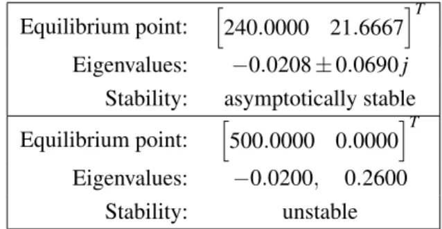
! A = " −d − θx2 −θx2 θx2 θx1− µ # x=xeq. (10) By using the model parameters of table 1, the results of table 2 are obtained.

4. Exact Linearization

System (1, 2) is not linearizable by performing a state transformation only. However, by the combined use of the transformations

(5)

Equilibrium point: $240.0000 21.6667%T Eigenvalues: −0.0208 ± 0.0690 j

Stability: asymptotically stable Equilibrium point: $500.0000 0.0000%T Eigenvalues: −0.0200, 0.2600

Stability: unstable

Table 2. Stability of the equilibrium points of the reduced model.

z = S(x) (12)

the following linear model is obtained

˙z = Az + Bv (13) with A = " 0 1 0 0 # B = " 0 1 # . (14)

The manipulated variable v in the transformed model is called ”virtual” because it has only mathematical existence, in opposition to u, that has the physical meaning of being the drug dosage actually applied to the patient. Equation (11) allows to compute the actual drug dose u such that between v and z there is a linear relationship to which linear control techniques may then be applied.

Proposition 1 The transformations performing linearization are β(x) = _θx 1 1x2(µ − d) (15) α(x) = −ds + d2x1+µ2x2+ (d − µ)θx1x2 (d − µ)θx1x2 (16) S(x) = " ϕ(x) s − dx1− µx2 # (17) withϕ(x) given by ϕ(x) = x1+x2−µ_{θ −}_µs+d_θ. (18)

Proof In [5] it is shown that the nonlinear system (3) with f (x0) =0 and scalar input

u is feedback linearizable around the equilibrium x0 if and only if the distributions Di

defined by

Di=span

&

g(x),adfg(x),...,adi−1f g(x)

'

(6)

verify the two following conditions:

dimDn(x0) =n, (20)

D_n−1is involutive around x0. (21)

In relation to the model (3) with f and g given by (4) and (5), the first condition results in dimD2(x) = rank $ g(x) adfg(x) % =βk c x2rank " x1 s − µx1 −x1 −s + dx1 # =2, for x1,x2$= 0 and µ $= d (22)

and hence dimD2(x0) = 2. The second condition is also verified because D1 =

span{g(x)} is involutive since the Lie bracket [g,g] = 0 ∈ D1. The model is therefore

feedback linearizable.

Since the conditions on Diare satisfied, there exists ( [5]) a functionϕ(x) that verifies

the following three conditions:

ϕ(x0) =0 (23)

&dϕ,adkfg'(x) = 0, k = 0,1,...,n − 2 (24)

&dϕ,adn−1f g'(x0)$= 0. (25)

In terms ofϕ(x), the linearizing transforms yielding (14) around the equilibrium state x0

are given by [5]: α(x) = −(LgLn−1f ϕ(x) )₋₁ Lnfϕ(x) (26) β(x) =(LgLn−1_f ϕ(x) )₋₁ (27) zi=Li−1f ϕ(x), i = 1,2,...,n. (28)

The function 18 satisfies the three conditions, in particular

1. Computingϕ(x) at the equilibrium x0given by point (9) yieldsϕ(x0) =0;

2. &dϕ,g' = ∂ϕ(x)_∂x g(x) = 0;

3. &dϕ,[ f ,g]' =∂ϕ(x)_∂x [f ,g] =βk_c(d − µ)x1x2$= 0, for x = x0.

(7)

The expression (18) forϕ(x) is obtained by noting that Condition 2 may be written as * ∂ϕ ∂x1 ∂ϕ ∂x2 +" 1 −1 # βk c x1x2=0 (29)

and hence implies thatϕ(x) satisfies the partial differential equation ∂ϕ

∂x1 =

∂ϕ

∂x2 (30)

whose solution is given by any differentiable functionΦ of argument x1+x2:

ϕ(x1,x2) =Φ(x1+x2). (31)

The simplest choice that also satisfies Condition 1 is given by (18). The expressions for α and β follow then in a straightforward way from (28).

With these transformations, the system in a region of state space around the equilib-rium (9) is transformed exactly in the linear system (14).

5. Control with known parameters

The problem of designing a control law for the linearized system is addressed here-after. The aim is to design a state feedback control law that generates the virtual manip-ulated variable v as a function of the transformed state z. More specifically, we want to design the vector of feedback gains K = [k1k2], the equilibrium value of v (denoted ¯v)

and the equilibrium ¯z = [¯z1¯z2]T of z corresponding to the a specified equilibrium of x, in

the control law:

v = ¯v− K!z (32)

where

!z:= z − ¯z. (33)

The equilibrium value of the control variable of the linear system verifies

A¯z+ B ¯v = 0. (34)

5.1. Equilibrium values

Assume that the concentration of infected cells x2is to be driven to a reference value

r and kept there. At the equilibrium defined by x2=r one has, by equating the derivatives

to zero in (1, 2)

(8)

and

x1=s − µr_d . (36)

In terms of the linearized system (that operates with transformed variables) this results in the equilibrium point ¯z = S( ¯x), i. e.:

" ¯z1 ¯z2 # = "_s−µr d +r +1θ(d − µ) −µs 0 # =T (r). (37) 5.2. LQ controller design

It is then possible to design a LQ controller, using the linearized dynamics, that keeps the system at the desired reference value r.

The transformation T (r) allows to compute the equilibrium point in terms of the variables (z1,z2). The controller is then designed by minimizing the quadratic cost

J =

+∞

!

0

zTQzz +ρv2dt (38)

where Qzandρ adjust the contribution of the variables z(t) and v(t). Since these variables

are virtual (corresponding to transformed states) it is difficult to develop heuristic choices of their values. Thus, it was decided to adjust the weights Qxfor the state variables x and

then compute the corresponding Qz. Using a linear approximation, it is concluded that

Qz=,∂S −1 ∂z -T Qx,∂S −1 ∂z -. (39)

These weights are ”tuning knobs” that allow the designer to adjust the relative impor-tance of the state variables and the drug usage.

6. Adaptive Control

In practice model parameters are not perfectly known. A possible approach to es-timate them is described hereafter and relies on a joint control Lyapunov function for both the control and estimation errors [7]. In the work reported only the adaptation of the infection parameterθ is considered.

6.1. Error equation

Letθ∗_{be the (unknown) true value of parameter}_{θ, assumed to be constant, and ˆθ its}

estimate. The estimation error !θ verifies

(9)

Differentiating (12) with respect to time and using the change of variable (11) yields ˙z =∂S_∂x.f (x,θ∗_{) +}_g(x,_θ∗₎/α(x, ˆθ)+β(x, ˆθ)v01. ₍₄₁₎

For the adaptive technique to be applied the equation error that relates the tracking error with the estimation error should be linear in !θ. For this sake, we do a first order expansion of bothα and β and neglect higher order terms:

α(x,θ∗₎_{≈ α(x, ˆθ) − !}_{α(x, ˆθ)!θ} ₍₄₂₎ β(x,θ∗₎_{≈ β(x, ˆθ) − !β(x, ˆθ)!θ} ₍₄₃₎ where ! α(x, ˆθ) =∂α ∂ˆθ = ds − d2_x 1− µ2x2 (d − µ)x1x2ˆθ2 (44) and !β(x, ˆθ) = ∂β ∂ˆθ= 1 ˆθ2₍_{d − µ)x}₁_x₂. (45)

With this approximation, and using the fact that ∂S ∂x {f (x,θ∗) +g(x,θ∗) [α(x,θ∗) +β(x,θ∗)v]} = Az + Bv (46) equation (41) becomes ˙z = Az + Bv +Ψ(x,v,θ)!θ (47) where Ψ(x,v,θ) := −∂S_∂xg(x, ˆθ)$!α(x, ˆθ) + !β(x, ˆθ)v%. (48) From this equation and using (32) and (34) the error equation is written as

˙!z= Ak!z+ Ψ(x,v,θ)!θ. (49) Since ∂S ∂x = " 1 1 −d −µ # (50) it follows that Ψ(x,v, ˆθ) = " 0 1 # v + ds − d2_x2 1− µ2x2 ˆθ . (51)

(10)

6.2. Adaptation law

In order to design an adaptation mechanism to adjustθ, consider the candidate Con-trol Lyapunov Function

V (!z,!θ) = !zT_P!z+1

γ!θ2 (52)

where P = PT _{is a positive definite matrix and}_{γ > 0 is a scalar design parameter.}

Differ-entiating V with respect to time and using (49) it follows that ˙V = !zT_(AT kP + PAk)!z+ !θ , 2ΨT_{(x,v, ˆ}_θ)P!z+2 γ˙!θ -(53) where Ak:= A − BK. (54)

For K such that Akis hurwitz (as it happens, for instance, if K is designed by solving the

LQ problem in section 5.1), there is Q = QT _{positive definite such that}

AT

kP + PAk=−Q. (55)

Using (55) and selecting ˙!θ such that

˙!θ = −γΨ(x,v, ˆθ)P_!z ₍₅₆₎

equation (53) becomes

˙V = −!zT_{Q!z! 0 ∀!z$= 0.} ₍₅₇₎

Using a standard argument based on La Salle’s Invariant Set Theorem it is then con-cluded that !z→ 0. Equation (56) implies the use of an adaptation law given by

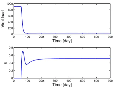
ˆθ(t) = −ˆθ(0)+ t ! 0 γΨT_{(x,v, ˆ}_θ)P!zdt ₍₅₈₎ or ˆθ(t) = ˆθ(0)+γ t ! 0 d2_x 1+µ2x2− ds − v ˆθ (p12!z1+p22!z2)dt. (59) Figure 1 shows a result obtained using adaptive controller.

7. Conclusions

It was shown that a reduced complexity nonlinear model for the HIV-1 infection can be controlled using adaptive nonlinear control methods. The approach followed com-bines exact linearization, LQ control and a joint control Lyapunov function for for the

(11)

0 100 200 300 400 500 600 700 0 200 400 600 800 1000 Viral load Time [day] 0 100 200 300 400 500 600 700 0 0.2 0.4 0.6 0.8 u Time [day]

Figure 1. Results with adaptive control.

tracking and estimation errors, to design the estimation law. Since this requires a linear dependence of the error equation on the estimation error, some approximations related to the linearizing transforms have to be performed.

The adaptation law considers only the tuning of the infection parameter. The same procedure may be extended to estimate the other parameters at the cost of a more cum-bersome algebra.

References

[1] F.L. BIAFORE and C.E. D’ATELLIS: Exact linearization and control of a HIV-1 predator-prey model. Proc. 2005 IEEE Eng. in Medicine and Biology 27th Annual Conf., Shanghai, China, (2005), 2367-2370.

[2] M.E. BRANDTand G. CHEN: Feedback control of a bioidynamical model of HIV-1. IEEE Trans. Biomedical Eng.,48(7), (2001), 754-759.

[3] C.-F. CHENGand C.-T. CHANG: Viral load analysis of a biodynamical model of HIV-1 with unknown equilibrium points. Proc. IEEE Conf. on Control Applica-tions, Taipei, Taiwan, (2004), 557-561.

[4] S. GEE, Z. TIAN and T. LEE: Nonlinear control of a dynamic model of HIV-1. IEEE Tran. Biomedical Eng.,52(3), (2005), 353-361.

(12)

[5] H. NIJMEIJERand A.VAN DERSCHAFT: Nonlinear Dynamical Control Systems. Springer-Verlag, 1990.

[6] A. PERELSONand P. NELSON: Mathematical analysis of HIV-1 dynamics in vivo. SIAM Review,41(1), (1999), 3-44.

[7] S. SASTRYand A. ISIDORI: Adaptive control of linearizable systems. IEEE Trans. on Automatic Control,34(11). (1989), 1123-1131.

[8] J.F. DE SOUZA, M. CAETANOand T. YONEYAMA: Optimal control applied to the antiviral treatment of AIDS. Proc. 39th IEEE Conf. on Decision and Control, Sydney, Australia, (2000), 4839-4844.

[9] Z. TIAN, S.S. GEand T.H. LEE: Globally stable nonlinear control of HIV-1 sys-tems. Proc. Amer. Control Conf., Boston, Massachusets, (2004).

[10] R. ZURAKOWSKI and A. TEEL: A model predictive control based scheduling method for HIV therapy. J. of Theoretical Biology,238 (2006), 368-382.