Analysis of multirate behavior in electronic systems

Jorge dos Santos

Freitas de Oliveira

Análise de Comportamentos Multi-Ritmo em

Sistemas Electrónicos

Analysis of Multirate Behavior in Electronic Systems

Tese apresentada à Universidade de Aveiro para cumprimento dos requisitos necessários à obtenção do grau de Doutor em Engenharia Electrotécnica, realizada sob a orientação científica do Doutor José Carlos Esteves Duarte Pedro, Professor Catedrático do Departamento de Electrónica,

Telecomunicações e Informática da Universidade de Aveiro, e sob a co-orientação científica do Doutor Adérito Luís Martins Araújo, Professor Auxiliar do Departamento de Matemática da Universidade de Coimbra.

Apoio financeiro da FCT e do FSE no âmbito do III Quadro Comunitário de Apoio.

Dedico este trabalho aos meus familiares e companheira, pelo incansável apoio e pela compreensão da minha constante indisponibilidade.

o júri

presidente Prof. Doutor João Carlos Matias Celestino Gomes da Rocha

professor catedrático da Universidade de Aveiro (em representação do Reitor da Universidade de Aveiro)

Prof. Doutor Thomas J. Brazil

professor of University College Dublin, Irlanda

Prof. Doutor José Carlos Esteves Duarte Pedro

professor catedrático da Universidade de Aveiro (orientador)

Prof. Doutor João José Lopes da Costa Freire

professor associado com agregação do Instituto Superior Técnico da Universidade Técnica de Lisboa

Prof. Doutor Nuno Miguel Gonçalves Borges de Carvalho

professor associado com agregação da Universidade de Aveiro

Prof. Doutor Adérito Luís Martins Araújo

professor auxiliar da Faculdade de Ciências e Tecnologia da Universidade de Coimbra (co-orientador)

agradecimentos Ao longo desta difícil mas estimulante etapa da minha vida intervieram, directa ou indirectamente, diversas pessoas e entidades às quais desejo expressar os meus sinceros agradecimentos.

Em primeiro lugar gostaria de agradecer ao Prof. Doutor José Carlos Pedro, na qualidade de orientador deste trabalho de doutoramento, pela sua inteira disponibilidade, por todo o apoio prestado, pelo óptimo ambiente de trabalho e pelo elevado grau de exigência que sempre pautou a sua actuação.

Gostaria também de agradecer ao Prof. Doutor Adérito Araújo, do

Departamento de Matemática da Universidade de Coimbra, pelos inúmeros conhecimentos que me transmitiu para a minha formação em matemática aplicada, e por ter aceite em participar como co-orientador deste

doutoramento.

Gostaria de agradecer à Universidade de Aveiro, ao Departamento de Electrónica, Telecomunicações e Informática e ao Instituto de

Telecomunicações, por terem fornecido os meios necessários para o desenvolvimento do meu trabalho.

Gostaria também de agradecer à Escola Superior de Tecnologia e Gestão de Leiria, pelo apoio prestado.

O apoio financeiro concedido pela Fundação para a Ciência e Tecnologia ao longo deste período sob a forma de bolsa de doutoramento é obviamente merecedor de um agradecimento especial.

Por último, agradeço aos colegas do Departamento de Engenharia

Electrotécnica da Escola Superior de Tecnologia e Gestão de Leiria, e a todos os meus amigos em geral, por toda a amizade, apoio e incentivo.

palavras-chave Circuitos RF Heterogéneos Não Lineares, Equações Diferenciais Não Lineares, Múltiplas Escalas de Tempo, Comportamentos Multi-Ritmo, Simulação Numérica.

resumo Esta tese insere-se na área da simulação de circuitos de RF e microondas, e visa o estudo de ferramentas computacionais inovadoras que consigam simular, de forma eficiente, circuitos não lineares e muito heterogéneos, contendo uma estrutura combinada de blocos analógicos de RF e de banda base e blocos digitais, a operar em múltiplas escalas de tempo.

Os métodos numéricos propostos nesta tese baseiam-se em estratégias multi-dimensionais, as quais usam múltiplas variáveis temporais definidas em domínios de tempo deformados e não deformados, para lidar, de forma eficaz, com as disparidades existentes entre as diversas escalas de tempo. De modo a poder tirar proveito dos diferentes ritmos de evolução temporal existentes entre correntes e tensões com variação muito rápida (variáveis de estado activas) e correntes e tensões com variação lenta (variáveis de estado latentes), são utilizadas algumas técnicas numéricas avançadas para operar dentro dos espaços multi-dimensionais, como, por exemplo, os algoritmos multi-ritmo de Runge-Kutta, ou o método das linhas. São também

apresentadas algumas estratégias de partição dos circuitos, as quais permitem dividir um circuito em sub-circuitos de uma forma completamente automática, em função dos ritmos de evolução das suas variáveis de estado. Para problemas acentuadamente não lineares, são propostos vários métodos inovadores de simulação a operar estritamente no domínio do tempo. Para problemas com não linearidades moderadas é proposto um novo método híbrido frequência-tempo, baseado numa combinação entre a integração passo a passo unidimensional e o método seguidor de envolvente com balanço harmónico.

O desempenho dos métodos é testado na simulação de alguns exemplos ilustrativos, com resultados bastante promissores. Uma análise comparativa entre os métodos agora propostos e os métodos actualmente existentes para simulação RF, revela ganhos consideráveis em termos de rapidez de

keywords Nonlinear Heterogeneous RF Circuits, Nonlinear Differential Equations, Multiple Time Scales, Multirate Behavior, Numerical Simulation.

abstract This thesis belongs to the field of RF and microwave circuit simulation, and is intended to discuss some innovative computer-aided design tools especially conceived for the efficient numerical simulation of highly heterogeneous nonlinear wireless communication circuits, combining RF and baseband analog and digital circuitry, operating in multiple time scales.

The numerical methods proposed in this thesis are based on multivariate strategies, which use multiple time variables defined in warped and unwarped time domains, for efficiently dealing with the time-scale disparities. In order to benefit from the different rates of variation of slowly varying (latent) and fast-varying (active) currents and voltages (circuits’ state variables), several advanced numerical techniques, such as modern multirate Runge-Kutta algorithms, or the mathematical method of lines, are proposed to operate within the multivariate frameworks. Diverse partitioning strategies are also introduced, which allow the simulator to automatically split the circuits into sub-circuits according to the different time rates of change of their state variables. Novel purely time-domain techniques are addressed for the numerical simulation of circuits presenting strong nonlinearities, while a mixed frequency-time engine, based on a combination of univariate time-step integration with multitime envelope transient harmonic balance, is discussed for circuits operating under moderately nonlinear regimes.

Tests performed in illustrative circuit examples with the newly proposed methods revealed very promising results. Indeed, compared to previously available RF tools, significant gains in simulation speed are reported.

Contents

List of Figures ... xvii

List of Tables... xix

List of Acronyms... xxi

Chapter 1 Introduction... 1

1.1 Motivation ... 1

1.2 Objectives... 3

1.3 Summary ... 3

1.4 Original Contributions... 4

Chapter 2 Background Material... 7

2.1 Introduction ... 7

2.2 Mathematical Model of an Electronic Circuit... 7

2.2.1 Lumped Problems ... 7

2.2.2 Distributed Devices ... 10

2.3 Transient Analysis... 12

2.3.1 Time-Step Integration ... 12

2.3.2 Runge-Kutta Methods ... 14

2.3.3 Conventional Transient Simulation Technique: SPICE ... 15

2.4 Steady-State Simulation Engines ... 15

2.4.1 Time-Domain Techniques... 16

2.4.2 Frequency-Domain Techniques ... 20

2.4.3 Comparisons... 25

Chapter 3 Advanced Simulation Techniques for Multirate RF Problems... 27

3.1 Introduction ... 27

3.2 Time-Domain Latency ... 28

3.2.1 State Variables with Different Rates of Variation... 28

3.2.2 Time-Step Integration using MRK Methods ... 30

3.3 Frequency-Domain Latency ... 32

3.4 Multirate Signals ... 33

3.4.1 Modulated Signals... 34

3.4.2 Mixed Frequency-Time ETHB Technique... 35

3.4.3 Quasiperiodic Signals... 36

3.4.4 Quasiperiodic Steady-State Solutions: the Multitone HB ... 37

3.5 Multivariate Formulation ... 40

3.5.1 Multivariate Representations... 40

3.5.2 MPDAE ... 42

3.5.3 Boundary Conditions... 43

3.5.4 Techniques for Computing the Solution of the MPDAE ... 46

3.6 Warped Time Formulation ... 50

Chapter 4 An Efficient Time-Domain Simulation Method ... 53

4.1 Introduction ... 53

4.2 Innovative Simulation Method ... 54

4.2.1 Bivariate Warped Time Formulation... 54

4.2.2 Envelope Transient over Shooting in a Warped Time Domain... 55

4.2.3 Shooting Based on Multirate Runge-Kutta Integration... 55

4.2.4 Active-Latent Partitioning Strategy... 56

4.3 Experimental Results... 58

4.3.1 Illustrative Application Example... 58

4.3.2 Numerical Simulation Results... 59

4.4 Conclusions ... 64

Chapter 5 An Efficient Multiple-Line Double Multirate Shooting Technique... 65

5.1 Introduction ... 65

5.2 Innovative Simulation Method ... 66

5.2.1 Multivariate and Warped Time Formulations ... 66

5.2.2 3-D Envelope Transient Oriented Technique... 68

5.2.3 2-D Bi-Periodic Boundary Value Problems ... 69

5.2.4 The Method of Lines ... 70

5.2.5 Multiple-Line Shooting Technique ... 71

5.2.6 Double Multirate Approach... 72

5.2.7 Antistiffness Strategy ... 72

5.2.8 Multipartitioning Strategy ... 75

5.3.1 Numerical Results for Simulations with Baseband Sinusoidal Regimes ... 77

5.3.2 Numerical Results for Simulations with Baseband EDGE Signals... 80

5.4 Conclusions ... 81

Chapter 6 Two Innovative Time-Domain Simulation Techniques ... 83

6.1 Introduction ... 83

6.2 Method of Lines MRK ... 86

6.2.1 Theoretical Formulation... 86

6.2.2 Active-Latent Partitioning Strategy... 88

6.2.3 Stiffness Occurrence ... 89

6.3 Mixed Method ... 91

6.3.1 Method of Lines MRK Merged with Envelope Transient over Shooting ... 91

6.3.2 Technical Details of Implementation ... 92

6.3.3 Active-Latent Partitioning Strategy... 95

6.4 Experimental Results... 95

6.4.1 Illustrative Application Example ... 95

6.4.2 Numerical Simulation Results... 96

6.5 Conclusions ... 97

Chapter 7 An Efficient Mixed Frequency-Time Simulation Method... 99

7.1 Introduction ... 99

7.2 Innovative Simulation Method... 101

7.2.1 Time-Domain Latency within the MPDAE Formulation... 101

7.2.2 Multitime ETHB ... 101

7.2.3 Multirate Multitime ETHB... 105

7.2.4 Circuit Partitioning Strategy... 107

7.3 Experimental Results... 108

7.3.1 Application Example... 108

7.3.2 Numerical Simulation Results... 109

7.4 Conclusions ... 113

Chapter 8 Conclusions and Future Work... 115

8.1 Conclusions ... 115

8.2 Future Work ... 116

List of Figures

Figure 2.1 Quasi-static model for a nonlinear capacitance ... 8

Figure 2.2 Nonlinear dynamic circuit example... 9

Figure 2.3 A lumped equivalent circuit to an infinitesimal section of a transmission line ... 11

Figure 3.1 Single step in a standard Runge-Kutta integrator ... 29

Figure 3.2 Micro and macrosteps in a multirate Runge-Kutta integrator ... 29

Figure 3.3 Multirate sampling technique ... 33

Figure 3.4 Envelope modulated signal in the univariate time... 41

Figure 3.5 Bivariate representation of the envelope modulated signal ... 41

Figure 3.6 Sawtooth path in the t1t2 plane for envelope modulated signals ... 44

Figure 3.7 Sawtooth path in the t1t2 plane for quasiperiodic signals... 45

Figure 3.8 Bivariate representation of the PM signal ... 51

Figure 4.1 Simplified power amplifier schematic used in wireless polar transmitters ... 58

Figure 4.2 Bivariate AM branch transistor source voltage ... 60

Figure 4.3 Univariate AM branch transistor source voltage in the digital clock time scale ... 61

Figure 4.4 Bivariate C1 capacitor voltage ... 61

Figure 4.5 Univariate C1 capacitor voltage in the slow envelope time scale ... 61

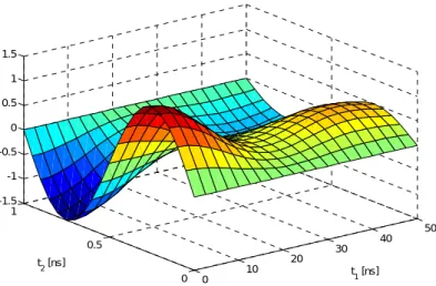
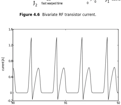
Figure 4.6 Bivariate RF transistor current... 62

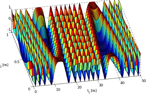
Figure 4.7 Univariate RF transistor current in the fast carrier time scale ... 62

Figure 4.8 Bivariate output voltage... 62

Figure 4.9 Univariate output voltage in the fast carrier time scale ... 63

Figure 5.1 Rectangular domains in the 3-D warped space... 68

Figure 5.2 Shooting strategies... 70

Figure 5.3 Double multirate uniform time grids to be used in the multiple-line shooting... 73

Figure 5.4 Antistiffness strategy ... 74

Figure 5.5 Bivariate AM branch MOSFET source voltage... 78

Figure 5.6 Univariate AM branch MOSFET source voltage in the digital clock time scale... 78

Figure 5.7 Bivariate drain voltage of the MOSFET RF switching-mode amplifier... 79

Figure 5.8 Univariate RF PA MOSFET drain voltage in the fast carrier time scale... 79

Figure 5.9 Univariate output voltage in the fast carrier time scale ... 80

Figure 5.10 Magnitude AM(t) of the EDGE test signal... 81

Figure 5.11 Phase PM(t) of the EDGE test signal... 81

Figure 6.1 Envelope modulated signals ... 84

Figure 6.2 Bivariate forms of the envelope modulated signals ... 85

Figure 6.3 Frequency-domain representation of two envelope modulated signals ... 86

Figure 6.4 Method of lines with MRK... 88

Figure 6.5 Mixed method ... 92

Figure 6.6 Simplified power amplifier schematic of a wireless polar transmitter ... 96

Figure 7.1 Two distinct state variables... 100

Figure 7.2 Bivariate forms of the state variables ... 102

Figure 7.3 Bivariate and univariate grids ... 106

Figure 7.4 Simplified resistive FET mixer used in wireless transmitters... 108

Figure 7.5 Bivariate RF transistor drain voltage ... 110

Figure 7.6 Bivariate output voltage... 110

Figure 7.7 Univariate RF transistor drain voltage... 110

Figure 7.8 Univariate output voltage... 111

Figure 7.9 Univariate baseband transistor source voltage... 111

List of Tables

Table 4.1 Computation times: explicit Runge-Kutta scheme of order 1 ... 60 Table 4.2 Computation times: explicit Runge-Kutta scheme of order 3 ... 60 Table 4.3 Computation times: explicit Runge-Kutta scheme of order 1 ... 63 Table 5.1 Computation times: RF polar transmitter PA baseband signals = 200 kHz sine waves.. 77 Table 5.2 Computation times: RF polar transmitter PA baseband signals = 2 MHz sine waves .... 80 Table 5.3 Computation times: RF polar transmitter PA baseband signals = EDGE test signals .... 82 Table 6.1 Computation times ... 97 Table 7.1 Computation times with K = 7 ... 112 Table 7.2 Computation times with K = 9 ... 112

List of Acronyms

AC alternating current AFM artificial frequency mapping AM amplitude modulation

APFT almost periodic Fourier transform

CMOS complementary metal-oxide semiconductor

CW continuous wave

DAE differential algebraic equations

DC direct current

DFT discrete Fourier transform

EDGE enhanced data rates for GSM evolution ETHB envelope transient harmonic balance FDTD finite-differences in time domain FET field effect transistor

FFT fast Fourier transform FM frequency modulation

GMRES generalized minimum residual GSM global system for mobile communications

HB harmonic balance

IDFT inverse discrete Fourier transform IFFT inverse fast Fourier transform LSI large scale integration

MDFT multidimensional discrete Fourier transform MFDTD multivariate finite-differences in time domain MOSFET metal-oxide semiconductor field effect transistor

MPDAE multirate partial differential algebraic equations MRK multirate Runge-Kutta

ODE ordinary differential equations PA power amplifier PLL phase-locked loop PM phase modulation PWM pulse-width modulation RF radio frequency RK Runge-Kutta SB spectral balance SoC systems-on-a-chip

SPICE simulation program with integrated circuit emphasis TD-ENV time-domain envelope following

VCO voltage-controlled oscillator VLSI very large scale integration

WaMPDAE warped multirate partial differential algebraic equations

2-D two-dimensional

Chapter 1

Introduction

1.1 Motivation

The increased use of digital signal processing and digital control techniques in current wireless transceivers, and the resulting combination of radio frequency (RF), baseband analog and digital technologies in the same circuit, created a new set of heterogeneous networks, and thus new challenges in terms of circuit simulation. In fact, both the necessity of providing increased levels of wireless systems’ functionality, and the need to improve the transmitters’ efficiency and linearity, have led to the extensive use of digital circuits, not only for signal processing purposes, but also for performing control operations. Current examples of these include receiver automatic gain control, transmitter output power control and look-up-table, or field-programmable-gate-arrays, based digital predistortion linearizers. This way, integrated systems-on-a-chip (SoC), combining RF and baseband analog and digital circuitry on modern complementary metal-oxide semiconductor field effect transistor (CMOS FET) technologies, are gradually reshaping current and upcoming wireless transceiver architectures.

An illustrative example where digital techniques have invaded the analog domain is the all-digital phase-locked loop (PLL) and transmitter chip recently demonstrated for GSM/EDGE hand-sets [66]. In this example, most of the conventional analog blocks were substituted by purely digital algorithms or mixed analog-digital circuits. That was the case of the power amplifier driver, in this design replaced by a high-speed digital-to-analog converter, appropriately named a digital-to-RF-amplitude converter. Other recent illustrative examples showing integration of digital techniques with traditional analog RF circuits are reported for example in [3], or [25]. The high heterogeneity and strong nonlinearity features of such networks brought a new range of challenges to circuit simulation. Because the RF, the baseband and the digital blocks are intricately mixed, it is not possible to adopt the circuit-level/system-level co-simulation methodology, in which some of the blocks are represented with a simplified system-level description, while the remaining (usually the

critical parts of the circuit) are simulated at the circuit-level, in a more or less independent way. Instead, a full circuit-level simulation technique is required, where we have to face a complex strongly nonlinear scenario, presenting heterogeneous state variables (node voltages and branch currents), evolving on widely disparate time scales.

The recent interest in envelope elimination and restoration power amplifiers [4], [18], [69], or wireless polar transmitters, has also conducted to new considerable difficulties that available RF simulators can not overcome. These are also clear examples of heterogeneous circuits where the circuit-level/system-level co-simulation technique is not applicable. In wireless polar transmitters, the amplitude, AM, and phase, PM, modulations are treated in two parallel branches. The PM branch is a traditional RF chain composed by a continuous wave (CW), sinusoidal RF carrier oscillator, a PM modulator and a highly efficient switching-mode power amplifier. Conversely, the AM path is a baseband chain whose signal is typically processed with digital over-sampling techniques [either with (sigma-delta quantizers) or without (pulse-width modulation) quantization noise shaping], which is then passed to the analog domain via fast switching power devices and a low-pass reconstruction filter. Thus, in such circuits, the RF and baseband (or even digital) circuitry are also intricately mixed. Moreover, the switching behavior of the AM power-supply modulator produces waveforms of very short rise and fall times that are extremely demanding on the number of harmonics, for a convenient frequency-domain representation. This advises the substitution of the traditional frequency-domain harmonic balance solvers (very popular in the RF and microwave community), by their time-domain rivals.

In summary, RF simulation has been led to an increasingly challenging scenario of heterogeneous broadband and strongly nonlinear wireless communication circuits, presenting a wide diversity of slowly varying and rapidly changing state variables. These circuits may also have excitation regimes with completely different formats and running on widely separated time scales [e.g., baseband information signals, AM signals, PM signals, RF carriers, digital clocks, pulse-width modulation (PWM) signals, etc.]. At present, none of the available RF tools, as the ones encountered in commercial packages, or the ones recently published in the literature, are capable of simulating this kind of circuits in an efficient way. The main reason for that is because RF tools do not perform any distinction between nodes or blocks within the circuit. Thus, since it is not possible to adopt the circuit-level/system-level co-simulation methodology, and a full circuit-level simulation technique is mandatory, all the blocks in the circuits are treated in the same way. This means that the same numerical algorithm is required to simultaneously compute the response of the digital blocks, the baseband analog blocks and the RF blocks. Obviously, this is not recommended at all in view of the fact that signals in different blocks have completely different features and evolve on widely disparate rates of change. For instance, it may be noted that, since time evolution rates of signals in different parts of a circuit may differ from three, or more, orders of magnitude,

and the sampling rate of the signals is dictated by the fastest ones, the application of the same numerical method to all the blocks will result in high inefficiency.

1.2 Objectives

In the above we have described the motivation for this thesis. We have showed that simulating some modern wireless communication systems is today a hot topic. In effect, serious difficulties arise when these nonlinear systems are highly heterogeneous circuits operating in multiple time scales. The main goal of this thesis is to develop new computer-aided design tools for the efficient numerical simulation of such circuits. In order to achieve this goal we had to go through the following intermediate steps:

• Analyze the circuits’ operation in order to identify and characterize their multirate behavior (stimuli heterogeneities, time-rate disparities of the state variables, existence of different time constants in distinct parts of the circuits, possible partition into active and latent sub-circuits, etc.);

• Get a general overview on the existing simulation tools, in order to examine the main characteristics of standard simulation methods (commonly used for computing the numerical solution of classic RF problems), and carefully study the most relevant advanced simulation techniques (available for computing the solution of multirate RF problems);

• Conceive innovative numerical simulation methods capable of simulating the circuits in an efficient way;

• Test the efficiency of the proposed numerical methods by applying them to illustrative application examples, and comparing the corresponding results with the ones obtained with available RF tools.

1.3 Summary

To fulfill the above stated objectives, this thesis is organized as follows.

After this brief introductory chapter, Chapter 2 provides some general background material on standard simulation techniques commonly used for computing the numerical solution of ordinary uni-rate problems. The chapter begins with the circuit equation formulation, in which some basic concepts and definitions for both lumped and distributed problems are given. Then, numerical integration algorithms well-suited for transient analysis are addressed, and finally time and frequency-domain techniques for computing periodic steady-state solutions are discussed.

Chapter 3 presents some advanced simulation techniques for computing the numerical solution of multirate RF problems. The chapter provides a general overview on the state of the art in multirate circuit simulation, in the sense that the most relevant contributions to this research field are reported and their capabilities discussed.

Chapter 4 is devoted to the discussion of a new computer-aided design tool, especially conceived for the efficient numerical simulation of highly heterogeneous and strongly nonlinear RF circuits, considered as running in two separated time scales. The proposed numerical method operates in a bivariate framework and uses modern multirate Runge-Kutta algorithms coupled with an envelope following technique to benefit from the circuits’ heterogeneity and stimuli time-rate disparities.

Since the efficiency of the method proposed in Chapter 4 degrades when more than two time scales are involved, Chapter 5 proposes an alternative powerful time-domain simulation technique to overcome that problem. The method proposed in this chapter is a robust simulation tool that is particularly suitable for highly heterogeneous and strongly nonlinear RF circuits running in three distinct time scales, and introduces an innovative multiple-line double multirate shooting technique operating within a 3-D framework.

Chapter 6 is dedicated to the discussion of two innovative time-domain techniques that operate within a bivariate framework of a periodic fast time scale and two aperiodic slow time scales, mixed in the same dimension. The methods are tailored for simulating strongly nonlinear RF circuits whose state variables are all fluctuating in the fast carrier time scale, but, in opposition, are presenting different rates of variation in the slow envelope time dimension. An alternative concept of time-domain latency is exploited in this chapter.

Chapter 7 describes a new mixed frequency-time technique, especially conceived for the efficient simulation of moderately nonlinear RF circuits. This new and efficient approach combines multitime envelope transient harmonic balance (ETHB) with a purely time-marching engine, to process some state variables in a bivariate mixed frequency-time domain, while others are treated in a single-time manner.

Finally, Chapter 8 concludes this thesis by summarizing its most relevant achievements, and pointing some future work directions as a continuation of this research.

1.4 Original Contributions

This thesis is believed to represent an important contribution to the RF and microwave circuit simulation area. The theoretical and experimental work carried out in this research have conducted to the development of some innovative computational tools, which demonstrated to be very powerful and appropriate to face the increasingly challenging simulation scenarios brought by modern wireless communication technologies.

The major contributions of this thesis can be summarized as the numerical methods described in Chapters 4, 5 and 7. The first and the second are innovative purely time-domain techniques, which allow the efficient simulation of highly heterogeneous RF circuits operating under strong nonlinear regimes. The third contribution consists in the development of a new mixed

frequency-time technique, which is more appropriate to deal with circuits presenting moderately nonlinearities.

We disseminated the main contributions of this research through the publication of papers in some major peer reviewed international conferences and journals. These are listed in the following.

Papers in International Conferences:

Oliveira, J. F., and J. C. Pedro, “A New Time-Domain Simulation Method for Highly Heterogeneous RF Circuits,” Proc. 37th European Microwave Conference, Munich, Oct. 2007, pp. 1161-1164.

Oliveira, J. F., and J. C. Pedro, “An Innovative Time-Domain Simulation Technique for Strongly Nonlinear Heterogeneous RF Circuits Operating in Diverse Time Scales,” Proc. 38th

European Microwave Conference, Amsterdam, Oct. 2008, pp. 1557-1560.

Papers in International Journals:

Oliveira, J. F., and J. C. Pedro, “An Efficient Time-Domain Simulation Method for Multirate RF Nonlinear Circuits,” IEEE Transactions on Microwave Theory and Techniques, vol. 55, no. 11, Nov. 2007, pp. 2384-2392.

Oliveira, J. F., and J. C. Pedro, “A Multiple-Line Double Multirate Shooting Technique for the Simulation of Heterogeneous RF Circuits,” IEEE Transactions on Microwave Theory and

Chapter 2

Background Material

2.1 Introduction

This chapter is intended to provide some background material on standard simulation techniques that may be used for computing the numerical solution of ordinary uni-rate problems. Section 2.2 is devoted to the circuit equation formulation, i.e., to the construction of a mathematical model that describes the operation of a generic electronic circuit. Then, the presentation of the various circuit analysis and simulation methods is organized by dividing them in two groups. The first one, described in Section 2.3, is devoted to the examination of the transient analysis of the circuits, in which the classic time-step integration techniques (the SPICE-like simulation engines) are focused. The second group, addressed in Section 2.4, is dedicated to the discussion of numerical algorithms for computing the steady-state solutions. We first examine some time-domain techniques, as shooting, or finite-differences in time domain (FDTD), to then analyze the most commonly used frequency-domain technique in the RF and microwave community: the harmonic balance (HB) method. A comparison between various aspects of the performance of the methods will be provided to make clear each of their strengths and weaknesses. Also, a comparison between the time and frequency-domain approaches will be made to elucidate the corresponding advantages and disadvantages.

2.2 Mathematical Model of an Electronic Circuit

2.2.1 Lumped Problems

The behavior of an electronic circuit can be described with a system of equations involving voltages, currents, charges and fluxes. This system of equations can be constructed from a circuit description using, for example, nodal analysis, which involves applying the Kirchoff current law to each node in the circuit, and applying the constitutive or branch equations to each circuit element.

v_C(t)

q_NL[v_C(t)] q(t) d/dt iC(t)

algebraic nonlinear

(voltage) (charge) (current)

linear dynamic

Figure 2.1 Quasi-static model for a nonlinear capacitance.

Under the quasi-static assumption, [27], [56], systems generated this way have, in general, the following form,

( )

t d

( )

t

( )

t , dt ⎡ ⎤ ⎣ ⎦ ⎡ ⎤ + = ⎣ ⎦ q y p y x (2.1)

where _x

( )

_t ∈Rn and _y

( )

_t ∈R stand for the excitation (independent voltage and current sources) n

and state variable (node voltages and branch currents) vectors, respectively. p y⎡_⎣

( )

t ⎤_⎦ stands for all memoryless linear or nonlinear elements, as resistors, nonlinear voltage-controlled current sources, etc., while models dynamic linear or nonlinear elements, as capacitors (represented as linear or nonlinear voltage-dependent electric charges), or inductors (represented as linear or nonlinear current-dependent magnetic fluxes).

( )

t

⎡⎣

q y ⎤⎦

The quasi-static assumption is invariably used when modeling nonlinear devices. In this approximation, all quantities in nonlinear circuit elements are assumed to be functions only of instantaneous values of the controlling variables [27], [56]. It should be noted that a quasi-static circuit element does not have to be memoryless. For instance, a capacitor is considered as quasi-static if its charge, and, consequently, its incremental capacitance, are only functions of the instantaneous voltage across its terminals. This way, its current-voltage dependence can be modeled by the cascade of a linear dynamic operator and an algebraic nonlinear function. Please see Figure 2.1.

The system of (2.1) is, in general, a differential algebraic equations’ (DAE) system. For

achieving an intuitive explanation of the mathematical formulation of (2.1), let us consider the basic illustrative example depicted in Figure 2.2. This circuit is composed of a current source connected to a linear inductance and two nonlinear circuit elements commonly used when modeling semi-conductor devices (a nonlinear capacitance and a nonlinear voltage-dependent current source). These nonlinearities are assumed as quasi-static and thus are described by algebraic constitutive relations of voltage-dependent charge and voltage-dependent current. A nodal analysis of this circuit leads to the following system of equations in the node voltage v_O

( )

t

L

v_O(t)

i_S(t) q_NL[v_O(t)] iNL[vO(t)]

i_L(t)

Figure 2.2 Nonlinear dynamic circuit example.

( )

( )

( )

( )

( )

( )

0 NL O L NL O S O L d i v t i t q v t i t dt d v t L i t dt ⎧ _{⎡ ⎤ + + ⎡ ⎤ =} ⎣ ⎦ ⎣ ⎦ ⎪⎪ ⎨ ⎪ _{+ ⎡− ⋅⎣ ⎤ =⎦} ⎪⎩ (2.2)

This system can be seen as a particular case (in ) of the DAE system of (2.1), in which the excitation vector, , and the vector of state variables,

2 R

( )

t x y

( )

t , are given by

( )

( )

,

( )

_{( )}

( )

. 0 S O L i t v t t t i t ⎡ ⎤ ⎡ ⎤ =_{⎢ ⎥} =_{⎢ ⎥} ⎣ ⎦ ⎣ ⎦ x y (2.3)

The DAE system of (2.1) may obviously be written in other forms. For instance, if we apply the chain differentiation rule to the dynamic term of its left hand side, we can obtain

( ) ( )

_{( )}

_{( )}

, d d t t t d dt = − ⎡⎣ ⎤⎦ q y y x p y y (2.4) or,

( )

t d

( )

t

( )

t

( )

, dt ⎡ ⎤ = − ⎡ ⎤ ⎣ ⎦ y ⎣ ⎦ M y x p y t ⎤⎦ (2.5) in which is usually known as the mass matrix. If this matrix is nonsingular, then the DAE system of (2.4) may degenerate into the following ordinary differential equations’ (ODE) system,

( )

t ⎡⎣ M y

( )

_{( )}

1

₍

_{( )}

_{( )}

₎

, d t t t t dt − = ⎡_⎣ ⎤_⎦ − ⎡_⎣ ⎤ y M y x p y _⎦ (2.6)

which can be rewritten in the classical form

( )

_{( )}

, d t t dt = ⎡⎣ ⎤⎦ y f t, y (2.7)

commonly used in the mathematical literature. When M y⎡_⎣

( )

t ⎤_⎦ is singular, the DAE system of (2.4) will not degenerate into a ODE system, but it is often possible to express it as a set of algebraic equations combined with a set of differential equations of the form of (2.7).

From the above we conclude that, in some cases, electronic circuits may be described by ODE systems instead of DAE systems. For example, if we return to the simple nonlinear dynamic circuit of Figure 2.2, and rewrite (2.2) as

( )

( )

_{( )}

_{( )}

_{( )}

( )

_{( )}

NL O O S NL O L O L O dq v dv t i t i v t i t dv dt di t L v t dt ⎧ = − ⎡ ⎤ − ⎪ ⎣ ⎦ ⎪ ⎨ ⎪ ₌ ⎪⎩ (2.8)

or, in its vector-matrix form, as

( )

( )

( )

( )

( )

( )

( )

0 0 O NL O S NL O L O L O dv t dq v i t i v t i t dt dv di t v t L dt ⎡ ⎤ ⎡ _{⎤ ⎢ ⎥ ⎡ ⎤} − ⎡ ⎤ − ⎢ ⎥_{⎢ ⎥ = ⎢} ⎣ ⎦ _⎥ ⎢ _{⎥ ⎢ ⎥ ⎢ ⎥} ⎣ ⎦ ⎢ _{⎥ ⎢ ⎥} ⎣ _{⎦ ⎣ ⎦} (2.9)

we can easily see that if dq_NL

( )

v_O dv_O ≠ then the mass matrix is nonsingular, and the circuit may 0 be described by an ODE system expressed in the classical form of (2.7), which, in this case, will simply result in

( )

( )

_{( )}

_{( )}

_{( )}

( )

_{( )}

1 1 O NL O S NL O L O L O dv t dq v i t i v t i t dt dv di t v t dt L − ⎧ _{⎡ ⎤} ⎡ ⎤ ⎪ =_{⎢ ⎥ ⎣} − ⎡_{⎣ ⎦⎤ − ⎦} ⎪ _{⎣ ⎦} ⎨ ⎪ = ⎪⎩ (2.10) 2.2.2 Distributed Devices

Practical RF and microwave circuits typically include linear time-invariant distributed devices such as nonideal transmission lines. For instance, when two distant points of a printed circuit board are connected by a conductor, the conductor will be (most of the times) physically implemented with a strip of metal which passes over, but is insulated from, a ground plane. This metal strip may be long enough so that the voltages and currents vary appreciably over its length. The metal strip, the insulator and the ground plane form an approximation to a transmission line, which is the most common distributed device used in modeling circuits. The distribution of the voltages and currents along the metal strip affects the circuit performance. So, since it cannot be seen as an ideal conductor, it is necessary to consider its nonideal behavior. The behavior of a transmission line can be computed by solving the wave equation system that describes the voltages and currents along its length,

L

G C

R

Figure 2.3 A lumped equivalent circuit to an infinitesimal section of a transmission line.

( )

( )

_{( )}

( )

( )

_{( )}

, , , 0 , , , 0 i z t v z t L Ri t z v z t i z t C Gv t z ⎧ ∂ ∂ z t z t + + = ⎪⎪ ∂ ∂ ⎨ ∂ ∂ ⎪ _{+ + =} ⎪ _{∂ ∂} ⎩ (2.11)

where v z t

(

,

)

and i z t are the voltage and current as a function of the position z along its length

( )

, and time t. R, L, G and C, are the series resistance and inductance, and shunt conductance and capacitance, per unit length, respectively. To solve for the entire time evolution of the currents and voltages in the transmission line, boundary conditions must be established at its ends, and the initial distribution of voltages and currents over its length must be known.

In order to simulate circuits with transmission lines, (2.11) must be numerically solved for each line. One standard algorithm for solving (2.11) consists in approximating the transmission line with several sections of a resistor-conductor-inductor-capacitor network, as the one shown in Figure 2.3, and then simulating the resulting nondistributed (lumped) equivalent circuit with standard simulation techniques. A second approach to simulate circuits with transmission lines can be obtained by taking advantage of the fact that only the voltages and currents at the ends, or terminals, of the line (z = 0 and z = l) have an effect on the rest of the circuit. In the case of linear time-invariant transmission lines, the terminal currents can be computed from the terminal voltages by convolution with impulse responses. This means that a term of the form

(

) ( )

, t t τ τ τd −∞ −

∫

h y (2.12)

in which h

( )

t is the matrix-valued impulse response of the linear time-invariant distributed devices in the circuit, will be included in the left hand side of (2.1) if this technique is adopted.

The lumped equivalent circuit approach, as also the convolution integral technique, can be both computationally expensive. Although they seem particularly simple to incorporate in time-domain circuit simulators, they involve substantial additional data. In the first case, this is due to the fact that the distributed devices commonly present in RF circuits can only be represented accurately by lumped equivalent models with a large number of nodes, which means that a large number of state variables is added to the circuit equation formulation of (2.1). In the case of the convolution

integral technique, the considerable amount of data results from the fact that to calculate currents using the convolution integral, the voltages for all past are needed. Since none of these two strategies are adequate to deal with distributed devices, in this thesis we have decided to adopt the compact DAE formulation of (2.1), or possibly (2.7), for the general time-domain mathematical description of the circuits.

In order to simulate circuits with transmission lines in an efficient way, a frequency-domain approach is mandatory. Indeed, if it is possible to perform numerical computations directly in the frequency-domain, then linear time-invariant distributed devices can be easily included. Since the distributed devices are considered as linear, superposition allows each frequency to be handled individually. Consequently, the frequency-domain constitutive relations between currents and voltages are still algebraic, just like in lumped devices, which means that it is relatively easy to develop frequency-domain models for distributed devices. To illustrate this point, consider the wave equation system at the frequency ω,

( )

( )

( )

( )

0 0 j t j t j t j t L R I z e V z e t z C G V z e I z e t z ω ω ω ω ⎧⎛ ∂ ₊ ⎞ ₊ ∂ ⎜ ⎟ ⎪ _{∂ ∂} ⎪⎝ ⎠ ⎨ ∂ ∂ ⎛ ⎞ ⎪_{⎜ + ⎟ +} ⎪_{⎝ ∂ ⎠ ∂} ⎩ = = (2.13)

in which the voltage and the current take the form V z e

( )

j tω and I z e

( )

j tω . V z and

( )

are complex phasors, and the system of (2.13) can be simplified to

( )

I z

(

) ( )

( )

(

) ( )

( )

0 0 j t j t j t j t R j L I z e V z e z G j C V z e I z e z ω ω ω ω ω ω ∂ ⎧ _{+ +} ⎪⎪ ∂ ⎨ _∂ ⎪ _{+ +} ⎪ ∂ ⎩ = = (2.14)

where the time derivatives were evaluated symbolically. This way, the partial differential system of (2.13) is converted into a simple ordinary differential system in space for the phasors. But, because only the terminal voltages and currents of the line affect the whole circuit in which it is inserted, (2.14) needs only to evaluated at z = 0 and z = l, and the line becomes described by a much simpler purely algebraic model.

Frequency-domain techniques are thus the right choice to handle distributed elements. These techniques differ form their time-domain rivals in many basic aspects and will be addressed later in Section 2.4.2.

2.3 Transient Analysis

2.3.1 Time-Step Integration

Let us consider the DAE system of (2.1), describing the behavior of a generic electronic circuit. Obtaining the solution to (2.1) over a specified time interval

[

t t0, Final

]

from a specific initial

condition , is what is usually known as an initial value problem, and computing such solution is frequently referred to as transient analysis. The most natural way to evaluate is to numerically time-step integrate (2.1) directly in time domain. One possible way to do so consists in simply converting the differential equations into difference equations, in which the time derivatives are approximated by appropriate incremental ratios. With this strategy, the nonlinear differential algebraic equations’ system of (2.1) is converted into a purely nonlinear algebraic system. For example, if we discretize the time t using a uniform grid (a set of a successive equally spaced time instants) defined as , and use the backward Euler rule (the popular implicit finite-differences scheme of order 1 [24]) to approximate the time derivatives of (2.1), we obtain

( )

t0 = y y₀

( )

t y 0 i t = + ⋅t i h

( )

( ) ( )

1

( )

, i i i ti h − − +q y q y = p y x (2.15)

where yi denotes an approximation to the exact solution y

( )

ti , and the parameter h= −ti ti−1 is

the time-step integration size. Small step sizes can provide a good accuracy in the simulation results but may conduct to large computation times. On the contrary, large step sizes will reduce the computation time but will definitely conduct to poorer accuracy. A good compromise between accuracy and simulation time is achieved when is dynamically selected according to the to solution’s rate of change. Once the solution

h

1

i−

y at the time instant ti−1 is known, the nonlinear

algebraic system given by (2.15) must be solved to compute . The iterative Newton-Raphson algorithm [19], [45], is usually employed to solve (2.15). In summary,

i

y

( )

t

y is evaluated for a set of successive time grid instants within the ti

[

t t0, Final

]

interval, beginning with the knowledge of

the initial condition y

( )

t₀ =y , and then solving the system of (2.15) for each time step. ₀

The above formulation derives directly from the intuitive idea that derivatives can be approximated, and thus simply replaced, by finite-differences schemes. Although this technique can be used to compute the transient response of a generic electronic circuit described by (2.1), there is as alternative strategy which is more often employed to find the solution of initial value problems. Such strategy consists in using initial value solvers, as linear multistep methods [16], [24], or Runge-Kutta methods [16], [24] (the most popular time-step integrators). Both classes of theses methods can provide a wide variety of explicit and implicit numerical schemes, with very distinct properties in terms of order (accuracy) and numerical stability. Consequently, for the same time-step length , solutions obtained with these methods can be extremely more accurate than the ones obtained with the backward Euler differentiation rule described above, which has order 1. Nevertheless, it must be noted that, instead of the backward Euler rule, an higher order finite-differences scheme could be used in (2.15). Because of substantial part of the research work described in this thesis is based on modern multirate Runge-Kutta schemes, we will restrict our presentation only on Runge-Kutta methods. Linear multistep methods will not be addressed here.

2.3.2 Runge-Kutta Methods

In view of the fact that the well-established theory of numerical integration is oriented toward the solution of standard ODEs, we will now consider the form of (2.7) for the mathematical description of a circuit’s operation. So, let us consider a generic initial value problem with state variables, expressed in its classical form by the system of (2.7) and the initial condition , i.e.,

n

( )

t0 = y y₀

( )

_{( )}

_{( )}

_{( )}

0 0 0 , , , _Final, n d t t t t t t t t dt = ⎡⎣ ⎤⎦ = ≤ ≤ ∈ y f y y y y . (2.16)

Definition 2.1: Runge-Kutta (RK) method. A standard s-stage RK method expressed by its Butcher tableau

(

b, A,c [24]

)

1 2 s c c c 11 12 1 21 22 2 1 2 s s s s s a a a a a a a a a_s (2.17) 1 2 s b b b

for obtaining the numerical solution of (2.16) at the time instant t1= + , is defined as [15], [24]: t0 h

(

0

)

1 0 1 , s i i i t h h b = + = +

∑

y y y k (2.18) where (2.19) 0 0 1 , , 1, s i i ij j j t c h h a i s = ⎛ ⎞ = ⎜ + + ⎟ = ⎝

∑

⎠ k f y k 2,…, .

The algorithm defined by (2.18), (2.19), allows the numerical solution at any generic time instant to be evaluated from its previous calculated value

i

y

i

t yi−1. If we have for ,

, then each of the in (2.19) is given explicitly in terms of the previously computed 0 ij a = j≥i 1, 2, , i= … s ki j

k , , and the method is then an explicit Runge-Kutta method. If this is not the case then the method is implicit and, in general, it is necessary to solve a nonlinear system of

1, 2, , 1

j= … i−

n s×

algebraic equations to simultaneously compute all the . In general, any iterative technique (e.g., fixed point iteration [19], [45], or Newton-Raphson iteration) may be used to solve the nonlinear system of (2.19).

i

k

Runge-Kutta methods are universally utilized for time-step integrating initial value problems, and differ from linear multistep methods in several aspects. Since they present a genuine one-step format, one of their main advantages is that there is no difficulty in changing the steplength in a dynamic time-step integration process (in opposition to multistep methods where considerable

difficulties may be encountered when we want to change steplength [24]). The automatic step size control is based on the estimation of local errors, for which diverse techniques can be used, such as extrapolation techniques, or embedded RK formulas. All theoretical and technical details of implementation of these techniques, as also many other aspects of the RK methods, as consistency, convergence, order conditions, numerical stability, etc., are out of the scope of this thesis. They can be seen, for example, in [15], or [24].

2.3.3 Conventional Transient Simulation Technique: SPICE

In the above we have seen that the most natural way of simulating an electronic circuit is to numerically time-step integrate, in time domain, the ordinary differential system describing its operation. So, it should be of no surprise that this straightforward technique was used in the first digital computer programs of circuit analysis and is still nowadays the most widely used numerical method for that purpose. It is present in all SPICE or SPICE-like computer programs.

SPICE (which means Simulation Program with Integrated Circuit Emphasis) was initially developed at the Electronics Research Laboratory of the University of California, Berkeley, in the early 1970’s. The real popularity of SPICE started with SPICE2 [32] in 1975, which was a much-improved program than its original version (SPICE1), containing several analyses (AC analysis, DC analysis, DC transfer curve analysis, transient analysis, etc.) and device models needed to design integrated circuits of that time. SPICE2 transient analysis used either the trapezoidal rule [24] or the Gear integration method [24], for the time-step integration of (2.1) with dynamic step size control.

Other versions of SPICE have been developed along the years and today many commercial simulators are based on SPICE. However, its application to RF circuits may cause some problems resulting from the specific behavior of RF systems. To understand that we must recall that RF signals are typically narrowband signals. This means that a data signal with a relatively low bandwidth is transmitted at a very high carrier frequency. To simulate a sufficient portion of the data signal a large number of carrier periods must be time-step integrated, and thus a very large number of time samples is required (a large amount of memory and computational time consumption). Some of the major limitations of SPICE transient analysis are overcome with the methods described in the following section.

2.4 Steady-State Simulation Engines

Although some simulation tools focus on transient analysis (SPICE-like simulation), the steady-state behavior of the circuits is typically of primary interest to RF and microwave designers. The main reason for that is because certain aspects of system performance are easier to characterize and verify in steady-state. For instance, distortion, noise, power, and transfer characteristics such as

gain, or impedance, are examples of quantities that are best measured, or simply only defined, when a circuit is in steady-state.

Time-step integration engines, as the ones described in the previous section, which were tailored for finding the circuit’s transient response, are not adequate for computing the steady-state. As seen, time-step integration is a numerical implementation for obtaining the solution of an initial value problem, because it evaluates for a set of successive time instants (time steps) from the knowledge of an initial condition . However, if the objective is the determination of the steady-state, there is no other way than to pass through the lengthy process of integrating all transients, and expecting them to vanish. In circuits presenting extremely different time constants, or high Q resonances, as is typically the case of RF and microwave circuits, time-step integration can be very inefficient. Indeed, in such cases frequencies in steady-state response are much higher than the rate at which the circuit approaches steady-state, or the ratio between the highest and the lowest frequency is very large. Thus, the number of discretization time steps used by the numerical integration scheme will be enormous, because the time interval over which the differential equations must be numerically integrated is set by the lowest frequency, or by how long the circuit takes to achieve steady-state, while the size of the time steps is constrained by the highest frequency component.

( )

t

y

( )

t0 y

Before beginning to present some common steady-state simulation techniques, it must be noted that there are several different kinds of steady-state behavior that may be of interest. The first one is

DC steady-state. Here the solution obviously does not vary with time. Stable linear circuits driven

by sinusoidal sources may exhibit a sinusoidal steady-state regime, which is characterized as being purely sinusoidal except, possibly, for some DC offset. If the steady-state response of a circuit consists of generic waveforms presenting a common period, then the circuit is said to be in periodic

steady-state. If a nonlinear circuit is excited by several periodic sources at uncommensurated

frequencies, the circuit will typically have a quasiperiodic steady-state regime. The computation of quasiperiodic responses, which consist of linear combinations of the sum and difference frequencies of a finite set of fundamental frequencies and their harmonics, will be discussed in the next chapter.

The periodic steady-state regime is the one that will be addressed in this section. In the following subsections we will briefly describe some standard steady-state simulation engines that compute the periodic steady-state solution in a much more efficient way than numerically integrating the circuit’s associated differential system from some arbitrary initial condition. Time-domain methods will be presented first. Then, frequency-Time-domain techniques will be addressed. 2.4.1 Time-Domain Techniques

Computing the periodic steady-state response of an electronic circuit involves finding the initial condition, y

( )

t₀ , for the differential system that describe the circuit’s operation, such that the

solution at the end of one period matches the initial condition, i.e., y

( )

t₀ = y

(

t₀+T

)

, where T is the period. Problems of this form, those of finding the solution to a system of ordinary differential equations that satisfies constraints at two or more distinct points in time, are referred to as

boundary value problems. In this particular case, we have a periodic boundary value problem that

can be formulated as

( )

( )

( )

,

( )

0

(

0

)

, 0 0 ,

( )

, n d t t t t t T t t t T t dt ⎡ ⎤ ⎣ ⎦ ⎡ ⎤ + = = + ≤ ≤ + ∈ ⎣ ⎦ q y p y x y y y (2.20)

or, in the classical ODE form, as

( )

_{( )}

_{( )}

₍

₎

_{( )}

0 0 0 0 , , , , n d t t t t t T t t t T t dt = ⎡⎣ ⎤⎦ = + ≤ ≤ + ∈ y f y y y y , T (2.21) where the condition y

( )

t₀ = y

(

t₀+

)

is known as the periodic boundary condition.

Solving (2.21) involves computing a numerical solution that simultaneously satisfies the differential system and the two point periodic boundary condition. Certainly, there is no shortage of mathematical literature describing methods for solving boundary value problems. However, certain methods have been found especially useful for electronic circuit problems. We will examine here the two standard time-domain alternatives that may be used for computing periodic steady-state responses of electronic circuits [21], [44]: the shooting method and the finite-differences in time

domain (FDTD) method.

2.4.1.1 The Shooting Method

The time-domain method most commonly used for numerically evaluating the periodic steady-state solution of an electronic circuit is the shooting method. Shooting solves boundary value problems by computing the solution to a succession of initial value problems with progressively improved guesses at an initial condition, which ultimately results in steady-state. In a circuit’s steady-state simulation, shooting begins by simulating the circuit for one period using some guessed initial condition (generally determined from a previous DC analysis). Then, the computed solution at the end of the period is checked, and if it does not agree with the initial condition, the initial condition is wisely modified. The circuit is then re-simulated with the adjusted initial condition, and this process is repeated until the solution after one period matches the initial condition.

In order to provide some mathematical details on the implementation of the shooting method, let us consider (2.21). Now suppose that we want to numerically time-step integrate the differential system in (2.21) with an initial value solver. As stated above, time-step integration is tailored for transient analysis, but is inadequate for computing steady-state responses. The problem comes from the fact that we don’t know a priori which initial condition y

( )

t₀ must be considered that will lead to the steady-state solution in the period T , i.e., that will satisfy the periodic boundary condition . So, we are trying to solve a boundary value problem with an initial value

( )

t0 =

(

t0+

)

solution technique. One possible way to convert the initial value solution procedure into a boundary value problem solver consists of guessing the initial estimate of y

( )

t₀ , or shooting for

, time-step integrating the differential system from

( )

t0

y t= until t0 t= + , comparing the t0 T

resulting with , and then wisely update the initial estimate. So, shooting is an iterative solver that uses an initial value technique to solve a boundary value problem. In the end, it relies on finding the solution of

(

t0+T

y

)

y

( )

t₀

( )

t0 =

(

t0+T

)

⇔

( ) (

t0 − t0+T

)

=0.

y y y y (2.22)

Let us now define y

(

t₀+T

)

= ⎡φ_⎣y

( )

t₀ ,T⎤_{⎦ and rewritte (2.22) as}

( )

t0 ,T

( )

t0 0

φ⎡_⎣y ⎤ −_⎦ y = , (2.23)

where φ is the state-transition function [21], [44]. An easy way to solve (2.23) consists in using the fixed-point iteration solver, which, in this case, would simply result in

[ ]1

_{( )}

[ ]

_{( )}

0 0 , . r r t φ t + T ⎡ ⎤ = ⎣ ⎦ y y (2.24)

However, shooting with the fixed-point iteration technique is obviously equivalent to integrating the original differential system from t= until all transients decay. So, it is generally a useless t0

technique because the convergence to the periodic steady-state solution may be extremely slow. A well known tactic to accelerate the route to steady-state, i.e., to accelerate the convergence of (2.23) to its solution, is the so-called shooting-Newton technique. As any other shooting technique, shooting-Newton is based on guessing initial conditions. However, it can take advantage of the fact that, although electronic circuits can be strongly nonlinear, their state-transition functions are usually quite linear. This means that slight perturbations on the initial condition (starting state) produce almost proportional perturbations in the subsequent time states. Taking this in to account, it is easy to conclude that (2.23) can be iteratively solved in an efficient way with the Newton’s method, which in this case will lead us to

[ ]

_{( )}

[ ]

_{( )}

( )

( )

_{( )} [ ]_{( )} [ ]

_{( )}

[ ]

_{( )}

0 0 0 1 0 0 0 0 0 , , 0 r r r r r t t t T t T t I t t t φ φ + = ⎡∂ ⎡_⎣ ⎤_⎦ ⎤ ⎡ ⎤_{− +⎢ − ⎥} ⎡ ₋ ⎤₌ ⎣ ⎦ _{⎢ ∂ ⎥} ⎣ ⎦ ⎣ ⎦ y y y y y y y y , (2.25)

where is the n identity matrix. The only entity of (2.25) that is difficult to compute is the derivative of the state-transition function (usually referred to as the sensitivity matrix). In order to compute this matrix we must take into consideration the chain differentiation rule. In fact, since in practice

I ×n

( )

t0 ,T

φ_{⎡⎣ y ⎤⎦ is nothing more than the numerical value , with being the total number}

of time steps in the interval

[

K

y K

]

0, 0

t t +T , which depends on the previous value , which, itself, depends on , and so forth, the sensitivity matrix can be given by

1 K− y 2 K− y

( )

( )

00 1 12 1 , . K K K K t T t φ ₋ − − ∂ ⎡ ⎤ 0 ∂ ∂ ∂ ⎣ _{⎦ = ⋅ ⋅ ⋅} ∂ ∂ ∂ y _{y y y} y y y ∂y (2.26)

It is easy to see that all the matrices in (2.26) can be individually computed along the time-step integration process. For concreteness, let us suppose that a standard Runge-Kutta method (2.18), (2.19), is being used to perform time-step integration on the consecutive iterations of the shooting method. If, for example, we want to evaluate the first matrix, then we have

1 1 0 0 . s i i i I h b = ∂ ∂ = + ∂

∑

∂ k y y y (2.27) Now, if we rewrite (2.19) as (2.28)

(

)

0 0 0 1 , , , s i i ij j i i j t c h h a t c h i s = ⎛ ⎞ = _⎜ + + _⎟= + = ⎝

∑

⎠ k f y k f Y 1, 2,…, , we obtain 0 0 , 0 , 1, 2, , i i i i t c h i s + ∂ ₌∂ _⋅∂ ₌ ∂ ∂ _Y ∂ k f Y y y y … . (2.29)

In an explicit Runge-Kutta method each one of the ∂ki ∂y may be evaluated in terms of 0

previously computed ∂k_j ∂y ₀, j=1, 2,… i, −1. In an implicit Runge-Kutta method all the ∂ki ∂y 0

in (2.29) must be computed simultaneously.

Although solving (2.25) and computing the sensitivity matrix may involve some extra computational cost, shooting-Newton converges to the steady-state solution much faster than the normal time-step integration procedure (shooting with fixed-point iteration). This is the reason why it is the time-domain steady-state engine most widely used in circuit simulation.

Beyond shooting-Newton, there is another well known technique that may be used to accelerate the convergence of the shooting method. Such technique is based on extrapolation methods, and will not be addressed in this thesis. All of its details of implementation can be seen in for example in [21].

2.4.1.2 FDTD

Finite-differences in time domain (FDTD) is an alternative technique that can be utilized to determine the solution of a boundary value problem, and thus may be used to compute the periodic steady-state response of an electronic circuit. FDTD methods consist in defining a time grid over the entire time interval, to then impose a discretization of the differential system, replacing its derivatives with finite-difference approximations. With this strategy, the differential system describing the circuit’s operation is converted into a nonlinear algebraic equations’ system, which can be solved iteratively. A brief explanation of the FDTD methods is provided in the following.

Let us consider (2.20). Let us also consider the discretization of the

[

t t₀, ₀+T

]

time interval defined by the grid

0 1 2 i1 i K 0 , i i i 1,