Fractional Order Modeling and GA Based Tuning for Analog Realization with Lossy Capacitors of a PID Controller

Abstract _{- In this paper, first it has been studied how the}

performance of a PID controller deteriorates when implemented with lossy capacitors in its analog realization. Thereafter it has been shown that the lossy capacitors can be effectively modeled by fractional order terms. Finally, a novel GA based method has been proposed to tune the controller parameters such that the original performance is retained even though realized with the same lossy capacitors. Simulation results have been presented to validate the usefulness of the technique.

Index Terms - _{Dielectric loss, Fractional order PID controller,}

Genetic Algorithm (GA), PID controller.

I. INTRODUCTION

ITH all of its lack of flexibilities, the classical PID controller still remains the most popular and widely employed controller in the industry mostly due to its simplicity. Therefore there has been an intense effort in the control system community to increase its flexibility so as to enable it to control a larger class of dynamic systems. One way of achieving this is to extend it to include fractional order integration and differentiation thereby making it a fractional order PID (PIλDμ) controller. A PIλDμ controller has the potential of not only outperforming conventional integer order PID controller but also of making it possible to control fractional order systems, distributed parameter systems, uncertain systems etc. [1].

In this article, an integer order PID controller has been designed for a 2nd order linear time-invariant system and it has been observed how its performance deteriorates when realized with an active analog circuit using lossy capacitors. Next it has been shown that the dielectric losses in the capacitors can be effectively modeled if the controller is assumed to be of fractional order. Thereafter a novel GA

Manuscript received August 24, 2008.

Bijoy K. Mukherjee is with the Department of Electrical Engineering, Asansol Engineering College, Asansol -713304, West Bengal, India. (e-mail: vj_bec@rediffmail.com)

Santanu Metia is with the Department of Electrical Engineering, B.P.Poddar Institute of Management & Technology, VIP Road, Kolkata-700052, West Bengal, India. (e-mail: metia_santanu@yahoo.co.in)

based tuning method in both time and frequency domains of this modeled PIλDμ controller gains have been proposed so that the original performance is retained with the same lossy capacitors in the analog realization. MATLAB simulation results have been given to justify the usefulness of the proposed method.

II. A BRIEF INTRODUCTION TO PIλDμ CONTROLLER The most common form of a fractional order PID controller is the PIλDμ controller [2], involving an integrator of order Ȝ and a differentiator of order ȝwhere Ȝand ȝ can be any real numbers. The transfer function of such a controller has the following form,

Gc(s) = KP +KI / sȜ+ KD sµ, (Ȝ, ȝ > 0). (1)

Clearly, classical PID controller is a special case of PIλDμ controller with Ȝ = 1, ȝ = 1. Classical PI and PD controllers can also be recovered from (1) by proper choice of Ȝ and ȝ values. It can be expected that the PIλDμ controller may enhance the systems control performance because of its potential enhanced flexibility. Another advantage of the PIλDμ controller is the possible better control of fractional order dynamical systems. As a matter of fact the PIλDμ controllers are also more robust than their classical counterparts due primarily to the presence of two extra degrees of freedom [2]. It is pointed out in [3] that a finite dimensional approximation of the fractional order controller is possible and it should be carried out in a proper range of frequencies of practical interest.

III. EFFECT OF CAPACITOR LOSS ON THE PIDCONTROLLER PERFORMANCE

A. Design and Analog Realization of a PID Controller

Consider a unity feedback control system as shown in Fig.1. The transfer function of the plant is taken as

9

6

.

3

1

)

(

₂

+

+

=

s

s

s

G

_P [4] and the band limited PID

controller is taken to be of the form,

Fractional Order Modeling and GA Based

Tuning for Analog Realization with Lossy

Capacitors of a PID Controller

Bijoy K. Mukherjee and Santanu Metia

1

)

(

+

+

+

=

D D I

P c

sT

s

K

s

K

K

s

G

(2)

Fig.1. Unity feedback system

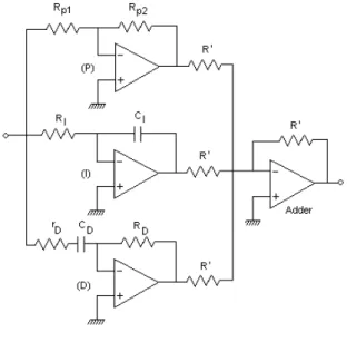
Following [5] the PID controller has been designed such that settling time is 0.3 sec and overshoot is 12.5%. The step response of the closed loop system is shown in Fig.2. The analog realization of the PID controller is shown in Fig.3 with the parameter values given in Table1. The actual realization taking into account the dielectric losses in the capacitors of the integral and derivative parts of the controller is shown in Fig.4 where Rp and Rs are the resistors representing the losses.

0 0.1 0.2 0.3 0.4 0.5 0.6 0.7 0.8 0.9 1 0

0.2 0.4 0.6 0.8 1 1.2 1.4

Step Response

Time (sec) A

m plitu d e

Fig.2. Step response of the closed loop system of Fig.1

Table 1: PID Controller Parameters

Parameter Value

KP KI KD TD

54.25 154.22 14.52 0.0482

Rp1 Rp2 RI CI RD CD rD R’

1 kΩ 54.25 kΩ 29.474 kΩ

0.22 μF 66 MΩ 0.22 μF 219.09 kΩ

10.0 kΩ

Fig.3. Analog realization of a PID controller

Fig.4. Analog realization of the integral and derivative parts considering dielectric losses in the capacitors

B. Effect of Capacitor Losses on the Performance of PID Controller

To observe the effect of capacitor losses on the performance of the PID controller the loss tangent of the capacitor is experimentally determined from measurement of phase difference between V and VR as shown in Fig.5 where R is a

known resistor and from the phasor diagram of Fig.6. The frequency of the source V is kept near to the natural frequency of the closed loop system. The experimental results are shown in Table2.

Fig.6. Phasor diagram corresponding to Fig.5 (b)

Fig.7. Oscilloscope plot of V (dotted) and VR (continuous)

Table 2. Experimental results for determination of loss tangent of the capacitor

φm 48.3582 deg

m

Z 295.74 kΩ

From Fig.6. o

m m m m Z R Z 317 . 5 sin cos

tan 1 − =

= −

φ φ

δ .

The following relations are obtained from [6]. C = ε0εr′, Rp

= 1/(ωε0εr″) and tan δ = εr″/εr′. Substituting the value of δ we

get, Rp = 2.6 MΩ. The quality factor of the capacitor is Qc =

ωRpC = 10.82 >10. Hence the equivalent series parameters

are = =

2 c p s Q R

R 22.2858 kΩ and

C

s

=

C

= 0.22 μF [7]. Substituting these values in the active circuits as shown in Fig.4 and Fig.3, the actual transfer function of the PID controller is obtained as,

) 5 . 22 ( ) 741 . 9 39 . 5 ( 251 . 356 ) ( 2 , ₊ + + = s s s s s

G_ca (3)

Table3. Time domain performance with Ideal and Actual PID Controllers

Specification Ideal PID Actual PID

tr 0.0924 sec 0.0891 sec

tp 0.1970 sec 0.2000 sec

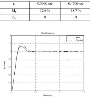
ts 0.3090 sec 0.4700 sec

Mp 12.6 % 18.7 %

ess 0 0

0 0.5 1 1.5

0 0.2 0.4 0.6 0.8 1 1.2 1.4 Step Response Time (sec) A mpl it u d e Ideal Practical

Fig.8. Step response due to ideal and actual PID controller

Actual controller Gc,a (s) yields the step response as shown

in Fig.8. In Table 3 is shown how different time domain specifications of the closed loop system get correspondingly changed.

IV. FRACTIONAL ORDER MODELING OF A LOSSY CAPACITOR Impedance of a lossy capacitor is given by,

2 2 2 2 2 2 2 1 1 1 1 ) ( C R C R j C R R C j R C j R j Z p p p p p p C _ω ω ω ω ω ω + − + = + × =

s s C j R ω −

=

(4)

From Fig.6, tan

δ

=

ω

R_sC_s

(5) Impedance of a lossy capacitor can be modeled in fractional order as, C j C e C j j Z j f

C α α

πα α _ω πα πα ω ω

ω cos 2 sin 2

) ( 1 ) ( 2 / − = =

= −

(6)

Comparing (6) with (4), 2_tan 1_(cotδ) π

α ₌ −

₍₇₎

The actual controller transfer function therefore can be modeled as fractional order PID controller as,

1 ) ( , = + + ₊ s T s K s K K s G D D I P f a c α

α (8) where α = 0.9409 (from 7) and KP, KI , KD and TD are same

0 0.5 1 1.5 0

0.2 0.4 0.6 0.8 1 1.2 1.4

Step Response

Time (sec) A

m plitu d e

Practical Fractional

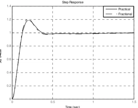
Fig. 9. Step response with modeled fractional order PID controller and the actual PID controller

V. GA BASED TUNING OF THE PIλDμ CONTROLLER GAINS A. Introduction to Genetic Algorithm

In 1975, GA was proposed firstly by Holland [9]. It is an optimization algorithm and applied to various fields, including business, science, and engineering. Based on the survival-of the-fittest strategy proposed by Darwin, this algorithm will eliminate unfit components to select the fittest component by man-made fitness function generation by generation.

Initialization

In the initialization, the first thing to do is to decide the coding structure. Coding for a solution, termed a chromosome in GA literature, is usually described as string of symbols from {0,1}. These components of the chromosome are then labeled as genes. The number of bits that must be used to describe the parameters is problem dependent.

Selection

GA uses proportional selection; the population of next generation is determined by n independent random experiments.

Crossover

Cross over is an important random operator in GA and the function of this operator is to generate a new ‘child’ chromosome from two ‘parents’ chromosomes by combining the information extracted from the parents.

Mutation

Mutation is another important component in GA, though it is usually conceived as a background operator. It operates independently on each individual by probabilistically perturbing each bit string. A usual way of mutation used in GA is to generate a random number between zero and one and then make a random change in the v-th element of the string with probability pm belonging to (0,1).

Encoding & Decoding

The design variables are mapped onto a fixed-length binary digit string, which are constructed over the binary alphabet

{0,1}, and is concatenated head-to-tail to form one long string referred as a chromosome. That is, every string contains all design variables.

The physical values of the design variables are obtained by decoding the string.

Fitness Function

In GA, the value of fitness represents the performance, which is used to rank the string, and the ranking is used to determine how to allocate reproductive opportunities. This means that individuals with higher fitness value will have higher probability of selection as a parent. Fitness thus is some measure of goodness to be optimized. The fitness function is essentially the objective function for the problem.

B. Tuning of the Controller Parameters in Time Domain

In the proposed method GA has been used to find the

D D I P K K T

K , , , values of the modeled fractional order controller as given in (8) such that the step response with this fractional order PID controller r(t_i)comes close to the response with the theoretical PID controller, g(t_i)as shown in Fig.2.

The time-domain fitness function is chosen as 2

0

)] ( ) (

[ _i

N

i

i r t

t g

J =

∑

−

=

(9) where g(ti)and r(ti)are unit step responses of the original

theoretical PID system and the modeled fractional order PID system respectively at the time instant

t

_i and

T T T

N f i

Δ −

= ( ) where T_f =final time, T_i =initial time,

=

ΔT sampling time.

0 0.1 0.2 0.3 0.4 0.5 0.6 0.7 0.8 0.9 1 0

0.2 0.4 0.6 0.8 1 1.2 1.4

Step Response

Time (sec) A

m plitu d e

Theoretical GA Tuned (time domain)

Fig.10. Step response with theoretical PID controller and the modeled fractional order controller tuned in time domain

C. Tuning of the Controller Parameters in Frequency Domain (Magnitude and Phase)

The frequency-domain fitness function for magnitude and phase are chosen as

2 0

]

)

(

)

(

[

_{i i}

i

j

R

j

G

J

f

ω

ω

ω

−

=

∑

=

and (10)

∑

= ∠ − ∠ = f i i

i R j

j G J ω

ω

ω

0 2 )] ( ) (

[ (11)

where

G

(

j

ω

_i

)

and

R

(

j

ω

_i

)

are the closed loop frequency-response values of the original theoretical PID controlled system and the modeled fractional order PID controlled system respectively at the

i

thfrequency

ω

_i.

0 0.1 0.2 0.3 0.4 0.5 0.6 0.7 0.8 0.9 1 0 0.2 0.4 0.6 0.8 1 1.2 1.4 Step Response Time (sec) A mpl itu d e Theoretical

GA Tunned (frequency domain, magnitude)

Fig.11. Step response with theoretical PID controller and the modeled fractional order controller tuned in frequency domain (magnitude)

0 0.1 0.2 0.3 0.4 0.5 0.6 0.7 0.8 0.9 1 0 0.2 0.4 0.6 0.8 1 1.2 1.4 Step Response Time (sec) A mpl itu d e Theoretical

GA Tunned (frequency domain,phase)

Fig.12. Step response with theoretical PID controller and the modeled fractional order controller tuned in frequency domain (phase)

Fig.11 and Fig.12 show that the theoretical performances can also be retained with the GA tuned fractional order PID controller if the tuning is done in the frequency domain considering the above mentioned objective functions. Fig.13 and Fig.14 show how the magnitude and phase of the frequency response data are matched. The parameter values of the tuned controllers as well as the resistor values for their analog realization with lossy capacitors are given in Table4.

-200 -150 -100 -50 0 50 Ma g nitu d e ( d B)

10-1 100 101 102 103 104 105 -270 -225 -180 -135 -90 -45 0 P h a s e ( d e g)

Bode Diagram

Frequency (rad/sec) Theoretical

GA Tunned (frequency domain, magnitude) Theoretical

GA Tunned (frequency domain, magnitude)

Fig.13. Frequency response with theoretical PID controller and the modeled fractional order controller tuned in frequency domain (magnitude)

-200 -150 -100 -50 0 50 Ma g nitu d e ( d B)

10-1 100 101 102 103 104 105 -270 -225 -180 -135 -90 -45 0 P h a s e ( d e g)

Bode Diagram

Frequency (rad/sec) Theoretical

GA Tunned (frequency domai, phase) Theoretical

GA Tunned (frequency domai, phase)

Fig.14. Frequency response with theoretical PID controller and the modeled fractional order controller tuned in frequency domain (phase)

TABLE4: PARAMETERS OF DIFFERENT GA TUNED CONTROLLERS

Parameters Time domain values Frequency domain values(mag) Frequency domain values (ph) KP KI KD TD 46.8689 152.8958 15.1769 0.0487 42.9769 159.7691 15.8607 0.0508 52.9508 143.0198 14.2261 0.0418 Rp1 Rp2 RI CI RD CD rD R’ 1.0 k 46.8689 k 29.729 k 0.22 μF 68.986 M

0.22 μF 221.36 k

10.0 k

1.0 k 42.9769 k

28.450 k 0.22 μF 72.094 M

0.22 μF 230.91 k

10.0 k

1.0 k 52.9508 k

31.782 k 0.22 μF 64.664 M

0.22 μF 190.00 k

10.0 k

All the above simulations have been obtained using Genetic Algorithm and Direct Search toolbox of MATLAB 7.1[10] and the results have been obtained after averaging over twenty Monte Carlo runs.

VI. CONCLUSION

this realization with lossy capacitors can be effectively modeled as a fractional order PID controller. Then a novel GA based tuning method of the controller parameters has been proposed so that the original performance of the PID controller is retained. Usefulness of the proposed method is justified with the help of MATLAB simulations.

ACKNOWLEDGMENT

All the simulations in the present work involving fractional order systems have been done using the CRONE control environment of Ninteger v.2.3, Fractional Control Toolbox of MATLAB.

REFERENCES

[1] Y.Q. Chen, “Ubiquitous Fractional Order Controls?” IFAC FDA06, Plenary Lecture, July 21, 2006.

[2] I. Podlubny. “Fractional Order Systems and PIλDμ Controllers”, IEEE Trans. Aut.Cont., vol.44, pp 208-214, 1999.

[3] A. Oustaloup, F. Levron, B. Mathieu, F.M. Nanot, “Frequency-band complex noninteger differentiator: characterization and synthesis”, IEEE Trans. Ckt.Syst.I, vol.47, pp 25-39, 2000.

[4] K. Ogata, “Modern Control Engineering”, 3rd Ed., Prentice Hall of India, New Delhi, 2000.

[5] G.C. Goodwin, S.F. Graebe and M.E. Salgado, “Control System Design” Prentice Hall of India, New Delhi, 2003.

[6] A.J. Dekker, “Electrical Engineering Materials”, Prentice Hall of India, New Delhi, 2002.

[7] R.A. De Carlo and P M. Lin, “Linear Circuit Analysis”, 2nd Ed., Oxford University Press, 2001.

[8] User and Programmer Manual, “Ninteger v.2.3”, 2005, Available: http://www.gcar.dem.ist.utl.pt/pessoal/dvalerio/ninteger/ninteger.htm. [9] J. Holland, “Adaptation in Natural and Artificial Systems”, University

of Michigan Press, Ann Arbor, Michigan, 1976.