EUROPEAN ORGANISATION FOR NUCLEAR RESEARCH (CERN)
Eur. Phys. J. C 77 (2017) 673
DOI:10.1140/epjc/s10052-017-5225-7
CERN-EP-2017-045 27th October 2017
Performance of the ATLAS track reconstruction
algorithms in dense environments in LHC Run 2
The ATLAS Collaboration
With the increase in energy of the Large Hadron Collider to a centre-of-mass energy of 13 TeV for Run 2, events with dense environments, such as in the cores of high-energy jets, became a focus for new physics searches as well as measurements of the Standard Model. These environments are characterized by charged-particle separations of the order of the
tracking detectors sensor granularity. Basic track quantities are compared between 3.2 fb−1
of data collected by the ATLAS experiment and simulation of proton–proton collisions pro-ducing high-transverse-momentum jets at a centre-of-mass energy of 13 TeV. The impact of charged-particle separations and multiplicities on the track reconstruction performance is discussed. The track reconstruction efficiency in the cores of jets with transverse mo-menta between 200 GeV and 1600 GeV is quantified using a novel, data-driven, method. The
method uses the energy loss, dE/dx, to identify pixel clusters originating from two charged
particles. Of the charged particles creating these clusters, the measured fraction that fail to be reconstructed is 0.061 ± 0.006 (stat.) ± 0.014 (syst.) and 0.093 ± 0.017 (stat.) ± 0.021 (syst.) for jet transverse momenta of 200–400 GeV and 1400–1600 GeV, respectively.
c
2017 CERN for the benefit of the ATLAS Collaboration.
Reproduction of this article or parts of it is allowed as specified in the CC-BY-4.0 license.
1 Introduction
The Large Hadron Collider (LHC) entered a new energy regime in 2015, at the start of Run 2, with proton–proton collisions at a centre-of-mass energy of 13 TeV. Events with TeV-scale jets showering in the detectors, or τ-leptons and b-hadrons that pass through multiple active layers of material, now occur at high enough rates to be studied in detail. These signatures also occur in potential new physics scen-arios including massive new resonances decaying to highly boosted bosons or top quarks whose decay
products are often reconstructed as a single jet [1]. In the cores of highly energetic hadronic jets and
τ-leptons, the average separation between highly collimated charged particles is comparable to the gran-ularity of individual sensors of the inner detector. This can create confusion within the algorithms used to reconstruct charged-particle trajectories, or tracks. Therefore, without careful consideration, the track reconstruction efficiency in these dense environments is limited, resulting in difficulties in identifying long-lived b-hadrons and hadronic τ-decays, or in calibrating the energy and mass of jets. To prevent
losses in efficiency, to increase the possibility of discovering new phenomena and to allow more detailed
measurements of the newly opened kinematic regime, a dedicated optimization for dense environments
was performed and deployed in the ATLAS [2] reconstruction for the start of Run 2. This updated
recon-struction provides superior physics performance, reduces the required computing resources, and is now the default used by ATLAS.
This paper first describes the ATLAS detector (Section2). Then, a general overview of the track
recon-struction algorithm (Section3) is given, focusing on the performance of charged-particle reconstruction
in dense environments at the start of Run 2. The data set utilized is described in Section4. The
qual-ity of the expected performance is evaluated in dedicated single-particle and dijet simulation samples
(Section5), and comparisons between simulation and data are performed in events with energetic jets.
Extending these mainly Monte Carlo (MC) simulation-based studies, a fully data-driven method is
intro-duced in Section6which probes the fraction of tracks lost in reconstruction, due to the high density and
collimation of charged particles in high-transverse-momentum1 (pT) jets. This is achieved by using the
ionization energy loss (dE/dx) in the pixel detector.
2 The ATLAS detector
The ATLAS experiment, a multipurpose particle detector at the LHC, covers almost the entire solid angle around the collision point, and consists of an inner detector (ID) tracking system surrounded by a thin superconducting solenoid magnet producing a 2 T axial magnetic field, electromagnetic and hadronic calorimeters, and a muon spectrometer incorporating three large toroid magnet assemblies.
The ID, shown in Figure1, provides position measurements for charged particles in the range |η| < 2.5 by combining information from three subdetectors. It consists of a cylindrical barrel region (full coverage
for |η| . 1.5) arranged around the beam pipe, and two end-caps. Disks in the end-cap region are placed
perpendicular to the beam axis, covering 1.5 < |η| < 2.5. Starting from the interaction point, the high-granularity silicon pixel detector segmented in r–φ and z (including the new innermost layer, the insertable
1ATLAS uses a right-handed coordinate system with its origin at the nominal interaction point (IP) in the centre of the detector and the z-axis along the beam pipe. The x-axis points from the IP to the centre of the LHC ring, and the y-axis points upwards. Cylindrical coordinates (r, φ) are used in the transverse plane, φ being the azimuthal angle around the z-axis. The pseudorapidty is defined in terms of the polar angle θ as η = − ln tan(θ/2). Angular distance is defined as ∆R ≡
B-layer (IBL) [3] added for Run 2) covers the vertex region and typically provides four measurements per track. The IBL has a mean radius of 33 mm and a typical IBL pixel has a size of 50 µm by 250 µm in the transverse and longitudinal directions with a sensor thickness of 200 µm. For the remaining three layers of the pixel system, located at mean radii of 50.5, 88.5, and 122.5 mm respectively, a typical pixel has a size of 50 µm by 400 µm in the transverse and longitudinal directions with a thickness of 250 µm. The pixel layer at a radius of 50.5 mm is referred to as the B-layer in this paper. The coverage in the end-cap region is enhanced by three disks on either side of the interaction point. The pixel detectors measure the charge collected in each individual pixel using the time over threshold (ToT) [4]. ToT is the time the pulse exceeds a given threshold and is proportional to the deposited energy.
Outside the pixel volume, the barrel of the silicon microstrip detector (SCT) consists of four double strip layers at radii of 299 mm to 514 mm, complemented by nine disks in each of the end-caps. A typical strip of a barrel SCT sensor has a length of 126 mm and a pitch of 80 µm. On each layer, the strips are parallel to the beam direction on one side and at a stereo angle of 40 mrad on the other. The information from the two sides of each layer can be combined to provide an average of four three-dimensional measurements per track. The SCT sensors are connected to binary read-out chips, which do not provide information about the collected charge. The silicon detectors are complemented by the transition radiation tracker
(TRT) [5], which extends track reconstruction radially up to a radius of 1082 mm for charged particles
within |η| = 2.0 while providing r–φ information. The raw timing information from its straw tubes is
translated into calibrated drift circles that are matched to track candidates reconstructed from the silicon detectors [5].
Figure 1:
Sketch of the barrel region of the ATLAS inner detector.
The solenoid is surrounded by sampling calorimeters. Calorimetry is provided by three distinct detectors
outside the ID volume. A lead/liquid-argon sampling electromagnetic calorimeter is split into barrel (|η|
barrel region (|η| < 1.7) and two end-cap copper/liquid-argon sections extend to higher pseudorapidity (1.5 < |η| < 3.2). Finally, the forward region (3.1 < |η| < 4.9) is covered by a liquid-argon calorimeter with a copper (tungsten) absorber in the electromagnetic (hadronic) section. In the outermost part, air-core toroids provide the magnetic field for the muon spectrometer. It consists of three layers of gaseous detectors: monitored drift tubes and cathode strip chambers for muon identification and momentum meas-urements for |η| < 2.7, and resistive-plate and thin-gap chambers for online event selection up to |η|= 2.4. A two-level trigger system, custom hardware followed by a software-based level, is used for online event selection and to reduce the event rate to about 1 kHz for offline reconstruction and storage.
3 ATLAS track reconstruction
The following provides an overview of primary-track reconstruction in the pixel and SCT detectors. After cluster creation, the primary-track reconstruction algorithm utilizes iterative track-finding seeded from combinations of silicon detector measurements, while additional methods are employed to recover non-prompt tracks. A staged pattern-recognition approach is used: a loose track candidate search, which allows a number of combinatorial track candidates, is followed by a stringent ambiguity-solver that com-pares and rates the individual tracks by assigning a relative track score to each track. This follows current approaches to track reconstruction first introduced in Ref. [6]. Further details, including a description of TRT track extensions, can be found in Ref. [7].
3.1 Clusterization
Charged-particle reconstruction in the pixel and SCT detectors begins by assembling clusters from the
raw measurements. A connected component analysis (CCA) [8] groups pixels and strips in a given
sensor, where the deposited energy yields a charge above threshold, with a common edge or corner into clusters. From these clusters, three-dimensional measurements referred to as space-points are created. They represent the point where the charged particle traversed the active material of the ID. In the pixel detector, each cluster equates to one space-point, while in the SCT, clusters from both sides of a strip layer must be combined to obtain a three-dimensional measurement.
The charge in a pixel sensor is often collected on multiple adjacent pixels. In the data set described in Section4, the average size of pixel clusters in the barrel is about two pixels in the r − φ plane and from one to three pixels in the longitudinal direction increasing with η. The total charge is proportional to the path length in the sensor and thus dependent on the incident angle of the particle. The particle’s intersection point with the sensor is determined from the pixels contributing to the cluster using a linear approximation
refined with a charge interpolation technique [9]. In dense environments, the spatial separation between
charged particles traversing the sensor is only a few pixels, and the CCA algorithm, at times, reconstructs only one cluster which includes energy deposits from multiple particles. Identifying such clusters reliably and quickly is paramount for an efficient charged-particle reconstruction in dense environments.
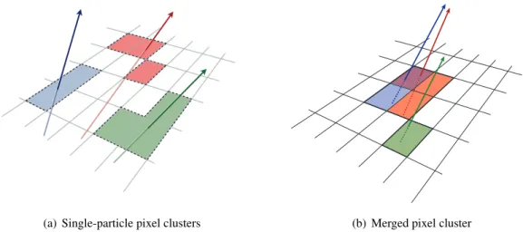
It is useful to introduce the several classes of clusters identified by either the "truth information", only available in simulation and referring to information at MC generator level, or reconstructed quantities in both collision data and MC simulation. Clusters created by charge deposits from one particle are called
single-particle clusters. Clusters created by charge deposits from multiple particles are called merged
information available in the track reconstruction algorithm described below, clusters which are compatible with a merged cluster can be identified. These are labelled identified as merged. Ideally, all clusters identified as merged are, in fact, merged clusters, and all merged clusters are identified as merged. Shared
clusters are those which are used in multiple reconstructed tracks but are not sufficiently compatible with
the properties of a merged cluster to be identified as merged by the reconstruction. Multiply used clusters - clusters used by multiple tracks - are either identified as merged or shared but not both.
(a) Single-particle pixel clusters (b) Merged pixel cluster
Figure 2: Illustration of (a) single-particle pixel clusters on a pixel sensor and (b) a merged pixel cluster due to very
collimated charged particles. Different colours represent energy deposits from different charged particles traversing
the sensor and the particles trajectories are shown as arrows.
3.2 Iterative combinatorial track finding
Track seeds are formed from sets of three space-points. This approach maximizes the possible number of combinations while still allowing a first crude momentum estimate. The impact parameters of a track seed, with respect to the centre of the interaction region, are estimated by assuming a perfect helical trajectory in a uniform magnetic field.
The purity, or fraction of seeds that result in good-quality tracks, varies significantly depending on which subdetector(s) recorded the space-points used in the seed. Therefore, seed types are considered start-ing with SCT-only, then pixel-only and finally mixed-detector seeds, representstart-ing the order of purity. A number of criteria are placed on the seeds to maximize purity: first and foremost seed-type-dependent momentum and impact parameter requirements. Also, the use of space-points in multiple seeds is care-fully controlled. Purity is further improved by requiring that one additional space-point is compatible
with the particle’s trajectory estimated from the seed. A combinatorial Kalman filter [10] is then used to
build track candidates from the chosen seeds by incorporating additional space-points from the remaining layers of the pixel and SCT detectors which are compatible with the preliminary trajectory. The filter creates multiple track candidates per seed if more than one compatible space-point extension exists on the same layer.
These criteria result in a very high efficiency for reconstructing primary particles (for example, the muon
reconstruction efficiency is greater than 99% [11]) and the removal of tracks created from purely
remain within the available CPU budget for event reconstruction. From approximately 13 space-point combinations created for an isolated charged particle traversing the entire ID, the time-intensive com-binatorial Kalman filter is, on average, called in its entirety 1.1 times. As all realistic combinations of space-points have been made, there are a number of track candidates where space-points overlap, or have been incorrectly assigned. This necessitates an ambiguity-solving stage.
3.3 Track candidates and ambiguity solving
In the ambiguity solver, track candidates considered to create the reconstructed track collection are pro-cessed individually in descending order of a track score, favouring tracks with a higher score. This design relies on having an appropriate track score definition that puts tracks into an order that scores more highly the candidates likely to correctly represent the trajectory of a charged primary particle.
The method used to determine the track score, discussed in the following, applies a robust approach based largely on simple measures of the track quality. Clusters assigned to a track increase the track score according to configurable weight fractions reflecting the intrinsic resolutions and expected cluster multiplicities in the different subdetectors. Holes2reduce the score. The χ2of the track fit is also
con-sidered to penalize candidates with a poor fit. Finally, the logarithm of the track momentum is concon-sidered to promote energetic tracks and suppress the larger number of tracks with incorrectly assigned clusters, which typically have a low pT.
After the track scores have been calculated, the ambiguity solver deals with clusters assigned to multiple track candidates. Clusters compatible with multiple track candidates are a natural consequence of having merged clusters in dense environments. High reconstruction efficiency is facilitated by the identification
of merged clusters, as explained in Section3.4. However, shared clusters, clusters used in multiple track
candidates which are not identified as merged, must be limited as they are a strong indicator of incorrect assignments.
To count shared clusters, a track candidate is only compared to those tracks previously accepted by the ambiguity solver. Clusters can be shared by no more than two tracks, giving preference to tracks processed first in the ambiguity solver. Also, a track can have no more than two shared clusters. A cluster is removed from a track candidate if it causes either the candidate or an accepted track to not meet the shared-cluster criterion. The track candidate is then scored again and returned to the ordered list of remaining candidates. Track candidates are rejected by the ambiguity solver if they fail to meet any of the following basic quality criteria:
• pT > 400 MeV,
• |η| < 2.5,
• Minimum of 7 pixel and SCT clusters (12 are expected),
• Maximum of either one shared pixel cluster or two shared SCT clusters on the same layer, • Not more than two holes in the combined pixel and SCT detectors,
2Holes are defined as intersections of the reconstructed track trajectory with a sensitive detector element that does not contain a matching cluster. These are estimated by following closely the track trajectory and comparing, within the uncertainties, the intersected sensors with the clusters on the track. Inactive sensors or regions, such as edge areas on the silicon sensors, are
• Not more than one hole in the pixel detector, • |dBL0 |< 2.0 mm,
• |zBL0 sin θ| < 3.0 mm,
where dBL0 is the transverse impact parameter calculated with respect to the measured beam-line position,
zBL0 is the longitudinal difference along the beam line between the point where dBL0 is measured and the
primary vertex3, and θ is the polar angle of the track. In the remainder of the paper, all studied tracks
fulfil these requirement. A simplified flow of track candidates through the ambiguity solver is shown in Figure3.
Calculate track scores
and Reject tracks with bad score
Order tracks according to score (process from highest to lowest) Input tracks Create stripped-down track candidate
Accept track candidate
or
Reject track candidate, if
too many holes
too few clusters
problematic pixel cluster(s)
or
Recover track candidate, if
too many shared clusters
(Neural network used to
identify merged clusters)
Output tracks Rejected
tracks
Fit tracks fulfilling minimum requirements
(Neural network used to
predict cluster positions)
Figure 3:
Sketch of the flow of tracks through the ambiguity solver.
3.4 Neural–network pixel clustering
To aid the ambiguity solver and minimize the loss of efficiency due to limitations on the number of shared clusters per track, an artificial neural network (NN) trained to identify merged clusters is used. The measured charge, which is proportional to the deposited energy, and relative position of pixels in the cluster can be used to identify merged clusters. Additional information about the particle’s incident
angle, provided from the track candidate, significantly improves the NN’s performance [13]. For merged
clusters created by two charged particles, the NN identification efficiency of this cluster as being created by two particles is about 90%. Merged clusters created by three charged particles are identified as such
with an efficiency of 85%. Only a few percent of single particle clusters are incorrectly identified as a
two-particle merged cluster and a negligible amount are identified as three-particle merged clusters. The NN is not able to distinguish clusters from exactly three and more than three charged particles. It is
3All events considered in this analysis are required to have at least one reconstructed primary vertex with at least two associated tracks [12]. Only tracks compatible with the primary vertex having the highest sum of the squared transverse momenta of its associated tracks are considered.
not possible for the NN to separate the energy deposits of each charged particle in an identified merged
cluster and subsequently divide it into multiple clusters. Unlike the Run-1 reconstruction algorithm [7],
the NN is consulted only when a cluster is used in multiple track candidates largely mitigating the impact of misidentification of merged clusters by the NN.
The inherent randomness of charged-particle interactions with thin silicon layers prevents the NN from
performing perfectly. For example, the emission of δ-rays causes difficulties as they can lead to bigger
clusters and larger energy deposits than expected from a single particle. These inefficiencies can be mit-igated by correlating information from consecutive layers of the pixel detector. In general, the separation between collimated charged particles increases as they travel outward through the ID. Therefore, if a pair of tracks uses a merged cluster on a given layer, then the inner layer is likely to contain a merged cluster as well. Furthermore, both clusters should be used by the same track candidates in this logic.
In summary, a cluster can be identified as merged in two ways. Either it is used by multiple track candid-ates and the NN identifies it as a merged cluster, or if two track candidcandid-ates compete for clusters on two consecutive layers, the cluster on the inner layer is identified as merged if the cluster on the outer layer is identified as merged. Clusters identified as merged are used by the competing track candidates without penalty. Clusters which are not identified as merged, shared clusters, can still be used in multiple tracks but with the penalty described in Section3.3.
3.5 Track fit
For track candidates fulfiling the requirements listed in Section3.3, a high-resolution fit is performed us-ing all available information. Fitted tracks which pass through the ambiguity solver without modification are added to the final track collection. Delaying the track fit until this stage minimizes the number of times the fitter is called, which is advantageous as it is a relatively CPU-intensive process.
For the high-resolution track fits, the position and uncertainty of each cluster is determined by additional
NNs [13]. They predict the positions where the charged particles intersected the sensor based on the
same input to the NN described in Section3.4. The predicted number of charged particles which created
the cluster determines the number of particle intersections the additional NNs predict. This decreases the discrepancy between the reconstructed cluster position and the cluster’s fitted track position at the detector surface, especially for merged clusters, resulting in more precise track parameters.
4 Data and Monte Carlo samples
Data from proton–proton collisions at √s = 13 TeV, collected during 2015 and corresponding to an
integrated luminosity of 3.2 fb−1, are used in this paper. Events are selected using triggers requiring a
single jet above various pT thresholds. The minimum jet trigger pT threshold is 100 GeV. The numbers
of events selected by the triggers were reduced by a factor depending on the instantaneous luminosity and
the jet pT threshold. This suppresses the number of low-pT jets while keeping all events with at least one
jet with pT > 450 GeV. Standard ATLAS data-quality requirements are applied to all data sets, ensuring
all detectors were operational.
The data are compared to a leading-order dijet MC sample generated with Pythia 8.186 [14] with the A14
generated with Herwig++ 2.7.1 [17], and Sherpa 2.1 [18] are also studied. For Herwig++, the UEEE5
tuned parameter set is used with the CTEQ6L1 PDF set [19] and for Sherpa, parameters corresponding
to the CT10 PDF set [20] are used. The ATLAS detector response is fully simulated [21] using the Geant
4 framework [22]. The average number of proton–proton interactions per bunch crossing (pile-up) was
approximately 15 during the 2015 data-taking period. The expected contribution from additional proton– proton interactions is accounted for by overlaying minimum-bias events simulated with Pythia 8. The MC samples are reweighted to match the distribution of the number of interactions per bunch crossing
and then reweighted to the inclusive jet-pT spectrum observed in collision data. In dense environments,
the impact of pile-up on the track reconstruction performance is small. The change in tracking efficiency
considering only one interaction per bunch crossing to an average pile-up of 40 in the dijet MC sample
for jets with a pTabove 200 GeV is below 0.3%.
In order to perform detailed simulation-based studies on event topologies with highly collimated particles, four large MC samples, with a single particle decaying into a set of nearby charged particles, are em-ployed. The initial particles have different lifetimes and decay multiplicities, and are generated with a uniform transverse momentum spectrum from 10 GeV to 1 TeV within |η| of 1.0. Topologies with two
highly collimated tracks are studied in a simulated ρ → π+π− sample. Simulated decays of a single
τ-lepton to three charged hadrons (τ± → π+π−π±ν
τ) are used to study topologies with three charged
particles. To study the performance in topologies with higher charged-particle multiplicities, two
addi-tional samples are created; a sample containing all decays of a B0into multiple particles and a τ-lepton
decaying to a final state including five charged hadrons.
5 Track reconstruction performance in dense environments
This section first compares basic properties of tracks inside jets in data with those in simulated dijet
samples (Section5.2). Using truth-based quantities, Section5.3studies single-particle decays with
col-limated decay products. These relatively simple topologies allow the behaviour of the track reconstruction to be studied as a function of the momentum of the initial particle, and the spatial separation between the
tracks. Section5.4presents analogous results, but derived from a dijet MC sample of high-pTjets.
5.1 Classification
In simulation, tracks are classified using a truth-matching probability. It is the ratio of the weighted number of measurements originating, at least in part, from the same simulated particle, to the weighted number of all measurements used in a track. A subdetector-specific weight of ten for measurements in the pixel detector, five for the SCT and one for the TRT is used. These weights reflect the average number of expected measurements in each subdetector. A properly reconstructed track is required to have a truth-matching probability above 0.5. Such a requirement is imposed for all reconstruction efficiencies presented in this paper.
Faketracks are those which have a truth-matching probability below 0.5. Due to the careful pruning of
seeds, the majority of reconstructed fake tracks are from the misallocation of clusters from other particles to a track and not purely random combinations of clusters. The track reconstruction procedure described
in Section3results in a negligible number of fake tracks in dense environments. For jets with a pTabove
only one pp interaction per bunch crossing to an average pile-up of 40, this fraction increases by about 0.5%, still making it negligible. Consequently, fake tracks are not discussed in further detail.
Jets are reconstructed from topological clusters [23] of energy deposits in the calorimeter using the anti-kt
algorithm [24] with a radius parameter R= 0.4 and are selected requiring a minimum jet pTof 200 GeV
and |ηjet| < 2.5. Jets are corrected for the effects of non-compensating response in the calorimeter and inactive material by using energy- and η-dependent calibration factors, based on MC simulation and pp collision data. Additional corrections are applied to reduce the dependence of the jet energy measure-ment on the longitudinal and transverse structure of the jets and also to correct for jets that are not fully contained in the calorimeter [25].
5.2 Data and MC simulation comparison
This section gives an overview of basic properties of tracks inside jets. Data and MC simulation compar-isons establish fair agreement between the two.
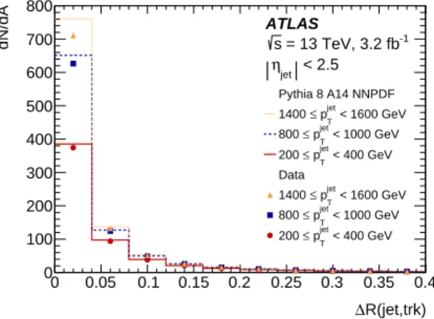
The average number of tracks per unit of angular area versus the angular distance from the jet axis in
data and MC events is compared in Figure4. The charged-particle density in jets increases linearly with
the logarithm of the jet momentum, which reflects the average number of tracks inside the jet. Moreover, most tracks are located within an angular distance of 0.05 from the jet axis. Jets in data tend to have a slightly wider distribution of reconstructed charged particles than those in simulation.
R(jet,trk) ∆ 0 0.05 0.1 0.15 0.2 0.25 0.3 0.35 0.4 dN/dA 0 100 200 300 400 500 600 700 800 ATLAS -1 = 13 TeV, 3.2 fb s < 2.5 jet η Pythia 8 A14 NNPDF < 1600 GeV jet T p ≤ 1400 < 1000 GeV jet T p ≤ 800 < 400 GeV jet T p ≤ 200 Data < 1600 GeV jet T p ≤ 1400 < 1000 GeV jet T p ≤ 800 < 400 GeV jet T p ≤ 200
Figure 4: The average number of primary tracks per unit of angular area as a function of the angular distance from
the jet axis. Data (markers) and dijet MC (lines) samples are compared in bins of jet pT showing the high density
in the cores of energetic jets.
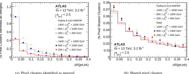
Due to the large number of collimated charged particles the number of multiply used clusters rises steeply
at small distances to the jet axis. Figure 5 shows the number of pixel clusters that are identified as
merged and the number of shared pixel clusters on the track for data and MC simulation versus the angular distance from the jet axis. The average number of shared pixel clusters remains relatively low compared to the number of clusters identified as merged, down to the smallest distances, because the
reconstruction algorithm identifies merged clusters with high efficiency, and these consequently are not
counted as shared. MC simulation and data show reasonable agreement in the individual bins of jet pT.
R(jet,trk)
∆
0 0.05 0.1 0.15 0.2 0.25 0.3 0.35 0.4
〉
N Pixel Clusters Identified as Merged
〈 0 0.2 0.4 0.6 0.8 1 1.2 ATLAS -1 = 13 TeV, 3.2 fb s < 2.5 jet η Pythia 8 A14 NNPDF < 1600 GeV jet T p ≤ 1400 < 1000 GeV jet T p ≤ 800 < 400 GeV jet T p ≤ 200 Data < 1600 GeV jet T p ≤ 1400 < 1000 GeV jet T p ≤ 800 < 400 GeV jet T p ≤ 200
(a) Pixel clusters identified as merged
R(jet,trk)
∆
0 0.05 0.1 0.15 0.2 0.25 0.3 0.35 0.4
〉
N Pixel Shared Clusters
〈 0 0.01 0.02 0.03 0.04 0.05 0.06 0.07 0.08 ATLAS -1 = 13 TeV, 3.2 fb s < 2.5 jet η Pythia 8 A14 NNPDF < 1600 GeV jet T p ≤ 1400 < 1000 GeV jet T p ≤ 800 < 400 GeV jet T p ≤ 200 Data < 1600 GeV jet T p ≤ 1400 < 1000 GeV jet T p ≤ 800 < 400 GeV jet T p ≤ 200
(b) Shared pixel clusters
Figure 5: The average number of (a) pixel clusters identified as merged and (b) shared pixel clusters on primary tracks (with a production vertex before the IBL) are shown as a function of the angular distance of the track from the
jet axis. Data (markers) and dijet MC (lines) samples are compared in bins of jet pT. The rise in both populations
at small distances from the jet axis is expected due to the increasingly dense environment.
and MC simulation versus the angular distance from the jet axis. For small distances the number of IBL
clusters shows a drop, explained by a residual inefficiency in assigning clusters to the appropriate track.
MC simulation and data agree within expectations in each of the individual jet pTbins. The overall lower
average number of IBL clusters on track in data is due to a not fully functional IBL detector module, which is not correctly considered in MC simulation.
R(jet,trk) ∆ 0 0.05 0.1 0.15 0.2 0.25 0.3 0.35 0.4 〉 N IBL Clusters 〈 0.9 0.92 0.94 0.96 0.98 1 1.02 ATLAS -1 = 13 TeV, 3.2 fb s < 2.5 jet η Pythia 8 A14 NNPDF < 1600 GeV jet T p ≤ 1400 < 1000 GeV jet T p ≤ 800 < 400 GeV jet T p ≤ 200 Data < 1600 GeV jet T p ≤ 1400 < 1000 GeV jet T p ≤ 800 < 400 GeV jet T p ≤ 200
Figure 6: The average number of IBL clusters on primary tracks (with a production vertex before the IBL) shown as a function of the angular distance of the track from the jet axis. Data (markers) and dijet MC (lines)) samples
are compared in bins of jet pT showing a slight drop at small distances explained by a residual cluster-to-track
assignment inefficiency.
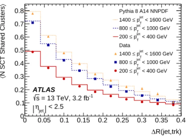
Although the SCT sensors are located at much higher radii than the pixel sensors, the expected number
of shared clusters is considerably larger than for the pixels as shown in Figure 7. This is due to the
coarser segmentation of the SCT strips in one dimension and the lack of charge information hindering the identification of merged SCT clusters. The average number of shared SCT clusters decreases with
the angular distance from the jet axis, correlated with the decrease in charged-particle density visible in
Figure4for data and MC simulation. In the studied jet-pTrange, the average number of SCT clusters on
tracks is approximately 7.7 with little variation with respect to angular distances from the jet axis. The
MC simulation agrees within expectations with data in the individual bins of jet pT.
R(jet,trk) ∆ 0 0.05 0.1 0.15 0.2 0.25 0.3 0.35 0.4 〉 N SCT Shared Clusters 〈 0 0.1 0.2 0.3 0.4 0.5 0.6 0.7 0.8 ATLAS -1 = 13 TeV, 3.2 fb s < 2.5 jet η Pythia 8 A14 NNPDF < 1600 GeV jet T p ≤ 1400 < 1000 GeV jet T p ≤ 800 < 400 GeV jet T p ≤ 200 Data < 1600 GeV jet T p ≤ 1400 < 1000 GeV jet T p ≤ 800 < 400 GeV jet T p ≤ 200
Figure 7: The average number of shared SCT clusters for primary tracks with a production vertex before the IBL is shown as a function of the angular distance of the track from the jet axis. Data (markers) and dijet MC (lines)
samples are compared in bins of jet pT. Due to the lack of charge information and the coarse sensor dimensions,
the clusters cannot be readily identified as merged.
5.3 Performance for collimated tracks
Quantities such as cluster assignment and track reconstruction efficiencies can be studied using truth
information from simulation to elucidate the track reconstruction behaviour in the presence of highly collimated charged particles. This section utilizes the single-particle samples described in Section4.
Fig-ure8shows how the minimum separation between charged particles at the IBL sensor surfaces evolves
with the initial particle’s pT. For the same pT, the density of the decay products may differ significantly:
the lighter the initial particle, or the higher the multiplicity of its decay products, the smaller the dis-tance. The degradation of the track reconstruction performance is mainly driven by the distance between charged particles and the charged-particle multiplicity in their vicinity. The results presented hereafter are therefore representative of the reconstruction performance in many physics processes, provided these parameters are known. Throughout this section, unless otherwise noted, it is required that all charged particles are created before the IBL (production radius smaller than 29 mm) in all figures shown.
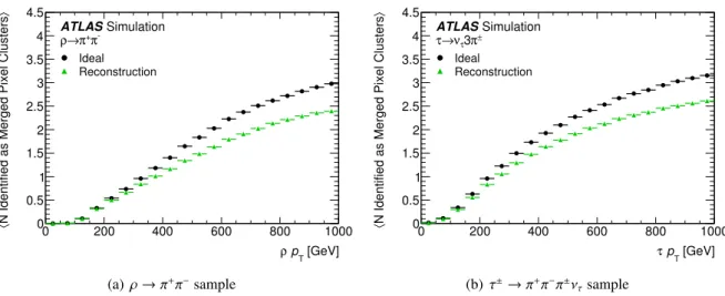
The average number of merged clusters is compared to the average number of clusters identified as merged
in Figure9for the single ρ and three-prong τ samples. The average charged-particle separation decreases
with increasing initial-particle pTleading to more merged pixel clusters as shown in the points labelled
Ideal. The average numbers of both the merged clusters and the clusters identified as merged fall to zero at the lowest initial-particle pT, confirming a low rate of false-positives. Both grow at a similar rate with
increasing initial-particle pT. The residual inefficiency of the pixel NN is apparent in a lower number
of clusters identified as merged compared to the ideal number of merged clusters at high initial-particle
pT. The reconstruction performance correlates directly with the multiplicity and distances at a given
[GeV] T p Initial Particle’s 0 200 400 600 800 1000 [mm]〉
Distance to Nearest Particle〈
2 − 10 1 − 10 1 10 ATLAS Simulation -π + π → ρ ± π 3 τ ν → τ X → 0 B ± 5X τ ν → τ
Figure 8: A comparison of the average minimum distance between charged decay products at the IBL sensor
surfaces as a function of initial particle’s pTfor single-particle samples.
[GeV] T p ρ 0 200 400 600 800 1000 〉
N Identified as Merged Pixel Clusters〈 0 0.5 1 1.5 2 2.5 3 3.5 4 4.5 ATLAS Simulation -π + π → ρ Ideal Reconstruction (a) ρ → π+π− sample [GeV] T p τ 0 200 400 600 800 1000 〉
N Identified as Merged Pixel Clusters〈 0 0.5 1 1.5 2 2.5 3 3.5 4 4.5 ATLAS Simulation ± π 3 τ ν → τ Ideal Reconstruction (b) τ±→π+π−π±ν τsample
Figure 9: A comparison of the average number of merged pixel clusters expected for truth particles from simulation and pixel clusters identified as merged used in reconstructed tracks is shown as a function of the ρ and three-prong
τ (τ → π+π−π±ν
τ) transverse momentum. Ideal represents the true number of merged clusters, which would be
obtained as the number of identified merged clusters in the case of perfect performance. It is required that the stable charged particles are created before the IBL.
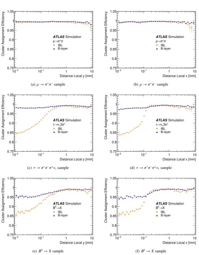
Merged clusters failing identification can result in shared clusters, which (as explained in Section3.3) need to be limited. To study possible inefficiencies of the reconstruction algorithm, the cluster assignment
efficiency is shown in Figure 10as a function of the minimum truth particle separation at the sensor’s
surface for the first two layers of the pixel detector. It is defined as the fraction of clusters created by a particle that are then used on the reconstructed track of said particle. With the closest truth particle
separated by 400 µm at the IBL, the cluster assignment efficiency at this layer is in excess of 99% for
the ρ and three-prong τ samples, and 98% for the B0 samples. When going to smaller separations,
individual clusters start to merge and eventually only a single merged cluster remains. Since in the simpler
topology ρ → π+π− the cluster has to be assigned to a maximum of two tracks, the cluster assignment
efficiency is 99% down to the smallest distances shown. In case of the B0 and three-prong τ decays,
several daughter particles are likely to contribute to a merged cluster. The NN described in Section3.4
lacks the ability to distinguish between merged clusters from more than three particles and those from
exactly three particles [13]. Also, the track reconstruction algorithm limits the number of tracks using
the same cluster without penalties to three. As a result, at much smaller particle separations, the cluster
assignment efficiency is limited in the B0and three-prong τ samples. The case of more than three charged
particles contributing to a pixel cluster in the B0decay results in an additional assignment inefficiency on the B-layer.
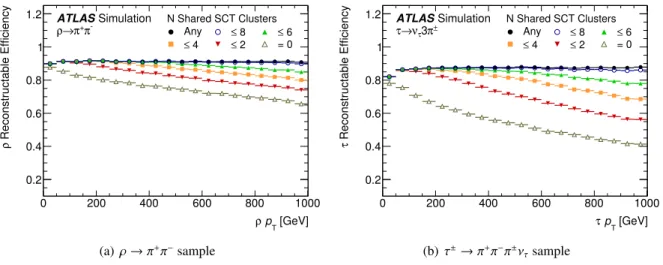
Regardless of how well the ambiguity solver identifies merged pixel clusters and assigns them to tracks,
a substantial inefficiency remains at high initial-particle momenta due to the necessary limitations on
shared SCT clusters. Figure11 shows the reconstructable efficiency of the ρ and three-prong τ decays
utilizing MC truth information. This is defined as the efficiency to be able to reconstruct all of the charged decay products from a given resonance having satisfied the cluster multiplicity requirements defined in
Section 3.3. All merged pixel clusters are assumed to have been identified, so for a fixed maximum
number of allowed shared SCT clusters, this represents the maximum achievable reconstruction efficiency.
The loss in efficiency is exacerbated by increasing charged-particle multiplicities as in the three-prong τ
sample. This limit is fixed at two shared clusters. The efficiency improvement obtained from loosening this limit is not sufficient to justify the associated increase in the proportion of fake tracks. In simulated events with several jets, the inclusive number of fake tracks increases by 25% when loosening the limit to three shared clusters.
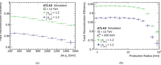
Finally, the per-track reconstruction efficiency is shown in Figure 12 as a function of particle pT and
production radius. The production radius is defined as the radial distance of the decay of the parent particle from the beam axis. The efficiency degrades with increased multiplicity. The visible inefficiency in all samples at low initial-particle pTis due to inelastic interactions, such as hadronic interactions. At
higher transverse momentum of the initial particle, a decrease in efficiency is driven by the increasingly
collimated nature of the decay products. A decrease in efficiency is also seen with a increasing production radius as the charged particles arrive at each active layer with less average separation. The requirement on the total number of clusters for track reconstruction leads to discrete drops in efficiency at each active layer.
5.4 Performance for tracks in jets
In the previous sections, the performance in simple topologies is discussed. These samples are crucial for understanding the effects of charged-particle separations and multiplicities on the performance, but they
Distance Local y [mm]
2 −
10 10−1 1 10
Cluster Assignment Efficiency
0.75 0.8 0.85 0.9 0.95 1 1.05 ATLAS Simulation -π + π → ρ IBL B-layer (a) ρ → π+π− sample Distance Local x [mm] 2 − 10 10−1 1 10
Cluster Assignment Efficiency
0.75 0.8 0.85 0.9 0.95 1 1.05 ATLAS Simulation -π + π → ρ IBL B-layer (b) ρ → π+π− sample Distance Local y [mm] 2 − 10 −1 10 1 10
Cluster Assignment Efficiency
0.75 0.8 0.85 0.9 0.95 1 1.05 ATLAS Simulation ± π 3 τ ν → τ IBL B-layer (c) τ → π+π−π±ν τsample Distance Local x [mm] 2 − 10 −1 10 1 10
Cluster Assignment Efficiency
0.75 0.8 0.85 0.9 0.95 1 1.05 ATLAS Simulation ± π 3 τ ν → τ IBL B-layer (d) τ → π+π−π±ν τsample Distance Local y [mm] 2 − 10 −1 10 1 10
Cluster Assignment Efficiency
0.75 0.8 0.85 0.9 0.95 1 1.05 ATLAS Simulation X → 0 B IBL B-layer (e) B0→ X sample Distance Local x [mm] 2 − 10 −1 10 1 10
Cluster Assignment Efficiency
0.75 0.8 0.85 0.9 0.95 1 1.05 ATLAS Simulation X → 0 B IBL B-layer (f) B0→ X sample
Figure 10: For the ρ (top), three-prong τ (middle), and B0(bottom) samples, the efficiency with which reconstructed
clusters are properly assigned to a track is shown for the two innermost pixel layers (IBL and B-layer) as a function of the minimum truth-particle separation in local y (left) and x (right), corresponding to the pixel dimensions longitudinal and transverse to the beam axis. It is required that the stable charged particles are created before the IBL.
[GeV] T p ρ 0 200 400 600 800 1000 Reconstructable Efficiency ρ 0.2 0.4 0.6 0.8 1 1.2 ATLAS Simulation -π + π → ρ N Shared SCT Clusters Any ≤ 8 ≤ 6 4 ≤ ≤ 2 = 0 (a) ρ → π+π− sample [GeV] T p τ 0 200 400 600 800 1000 Reconstructable Efficiency τ 0.2 0.4 0.6 0.8 1 1.2 ATLAS Simulation ± π 3 τ ν → τ N Shared SCT Clusters Any ≤ 8 ≤ 6 4 ≤ ≤ 2 = 0 (b) τ±→π+π−π±ν τsample
Figure 11: The reconstructable efficiency, defined as the efficiency to reconstruct all of the charged decay products
of the parent particle, is shown for the ρ and three-prong τ samples with various limits on the number of shared clusters allowed on a track candidate assuming all the merged pixel clusters have been identified as merged. It is required that the stable charged particles are created before the IBL.
[GeV]
T p
Initial Particle’s
0 200 400 600 800 1000
Track Reconstruction Efficiency
0.6 0.65 0.7 0.75 0.8 0.85 0.9 0.95 1 ATLAS Simulation -π + π → ρ ± π 3 τ ν → τ X → 0 B ± 5X τ ν → τ
(a) Efficiency versus initial particle’s pT
Stable-Particle Production Radius [mm]
0 10 20 30 40 50 60 70 80 90
Track Reconstruction Efficiency
0.5 0.6 0.7 0.8 0.9 1 ATLAS Simulation ± π 3 τ ν → τ X → 0 B ± 5X τ ν → τ
(b) Efficiency versus production radius
Figure 12: Single-track reconstruction efficiency is shown as (a) a function of the initial particle’s pT when it is
required that the parent particle decays before the IBL for the decay products of a ρ, three- and five-prong τ and a
B0and, (b) versus the production radius for the decay products of a three- and five-prong τ as well as a B0, where
As demonstrated in Section5.2, samples of dijet MC events do provide a reasonable description of jets in data. The following contains studies of the track reconstruction efficiency in these samples.
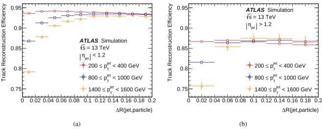
Figure13shows the charged-primary-particle reconstruction efficiency dependence on the angular
dis-tance of a particle to the jet axis for different jet η and pT ranges. All charged particles studied are
required to be created before the IBL. The efficiency drops rapidly towards the centre of the jet, where the charged-particle density is maximal. A slight decrease in efficiency towards the edge of the jet is consist-ent with an isolated-track efficiency that rises with charged-particle pT[26] and a decrease in the average
charged-particle pTwith distance from the jet core. The dependence of the efficiency on the jet pTand on
the production radius of the charged particle, where charged particles are not required to be created before
the IBL, is shown in Figure14. The decrease in efficiency with production radius is from two effects.
Firstly, particles created beyond the first active layers of the ID create fewer clusters. Secondly, with the shorter flight length to the next active layer, the average separation between particles is smaller compared to prompt decays, producing more merged clusters. The overall trend for all efficiencies shown is the same at all η. However, the loss in absolute efficiency is exacerbated at high |η|, while the degradation at small separations between a track and the jet axis is alleviated.
R(jet,particle)
∆
0 0.02 0.04 0.06 0.08 0.1 0.12 0.14 0.16 0.18 0.2
Track Reconstruction Efficiency
0.75 0.8 0.85 0.9 0.95 < 400 GeV jet T p ≤ 200 < 1000 GeV jet T p ≤ 800 < 1600 GeV jet T p ≤ 1400 ATLAS Simulation = 13 TeV s < 1.2 jet η (a) R(jet,particle) ∆ 0 0.02 0.04 0.06 0.08 0.1 0.12 0.14 0.16 0.18 0.2
Track Reconstruction Efficiency
0.75 0.8 0.85 0.9 0.95 < 400 GeV jet T p ≤ 200 < 1000 GeV jet T p ≤ 800 < 1600 GeV jet T p ≤ 1400 ATLAS Simulation = 13 TeV s > 1.2 jet η (b)
Figure 13: The efficiency to reconstruct charged primary particles in jets with (a) |η| < 1.2 and (b) |η| > 1.2 is
shown as a function of the angular distance of the particle from the jet axis for various jet pT for simulated dijet
[GeV]
T
Jet p
200 400 600 800 1000 1200 1400 1600
Track Reconstruction Efficiency
0.8 0.85 0.9 0.95 1 < 1.2 jet η > 1.2 jet η ATLAS Simulation = 13 TeV s (a) Production Radius [mm] 1 10 102
Track Reconstruction Efficiency
0.7 0.75 0.8 0.85 0.9 0.95 < 1.2 jet η > 1.2 jet η ATLAS Simulation = 13 TeV s > 200 GeV jet T p (b)
Figure 14: The track reconstruction efficiency is compared for charged primary particles in jets with |η| < 1.2
(|η| > 1.2) for the entire jet-pT range as a function of (a) the jet pT and (b) the production radius of the charged
particle for simulated dijet MC events, where charged particles are not required to be created before the IBL.
6 Measurement of track reconstruction e
fficiency in jets from data
Previous sections discuss the performance of the track reconstruction in dense environments based mainly on MC simulation. This section introduces a novel method to probe this performance in data. A meas-urement of the fraction of tracks lost in reconstruction due to the high density and collimation of charged particles in high-pTjets is presented for the subset of tracks with a B-layer cluster created by two charged
particles.
The dE/dx of a charged particle traversing the pixel sensor is measured from the charge collected in the clusters associated with the reconstructed track. With single particles and thin layers, one expects the
dE/dx measurements to approximately follow a Landau distribution [27]. A typical particle reconstructed
from an LHC collision is expected to be a minimum-ionizing particle (MIP). Thus, two particles contrib-uting to the same cluster are expected to deposit twice the energy of a single MIP. In the context of this paper, dE/dx is normalized to the material density, and it therefore has units of MeVg−1cm2.
As demonstrated in the previous sections, near the jet core the charged-particle density is high and particles can be highly collimated. The tracks of these particles are thus more likely to create merged
clusters, as shown in Figure5. By fitting the cluster dE/dx for reconstructed tracks near the core of the
jet, single-particle clusters can be statistically separated from merged clusters. The fraction of lost tracks can therefore be inferred from the number of times only one reconstructed track is associated with a
cluster dE/dx compatible with two MIPs. At truth-level, this fraction is defined as follows: the
denomin-ator is the number of truth particles passing the analysis selections (listed in Section6.1, and including
a pT > 10 GeV requirement), which have a B-layer cluster created by exactly two charged particles; the
numerator is the subset of these particles which failed to be reconstructed.
For the IBL, ToT is encoded in four bits. Eight bits are available in each of the remaining three pixel layers, which therefore provide an enhanced ToT resolution compared to the IBL, resulting in a superior
energy resolution. For this reason, the cluster dE/dx values corresponding to the B-layer are used in this
6.1 Track selection
To enhance the contribution of high-quality collimated tracks and suppress fake tracks to a negligible
number, additional track selections beyond those outlined in Section3.3are required for all tracks used
in this analysis:
• Exactly one pixel cluster per layer, • pT > 10 GeV,
• |η| < 1.2, • |dBL
0 |< 1.5 mm,
• |zBL0 sin θ| < 1.5 mm,
• Minimum of six SCT clusters.
6.2 Fit method
A measurement distribution of cluster dE/dx of tracks inside the jet core is fit using two dE/dx
tem-plate distributions: a single-track temtem-plate containing mainly tracks reconstructed from a single-particle cluster, and a multiple-track template mainly made up of tracks reconstructed from a merged cluster.
Both templates are derived directly from collision data or from simulation for the corresponding e
ffi-ciency measurements.
As verified in simulation, most highly collimated tracks are expected to be within ∆R(jet,trk) < 0.05
which then defines the jet core for this method. Outside the jet core, the contribution of collimated tracks is negligible, and therefore all tracks are expected to be reconstructed from a single-particle cluster. The single-track template is created using tracks reconstructed from clusters which are neither identified as
merged nor shared and that are well outside the jet core (∆R(jet,trk)> 0.1). The multiple-track template
is taken from tracks reconstructed from either B-layer clusters identified as merged or shared B-layer clusters inside the jet core. These multiply used clusters are likely to be merged clusters.
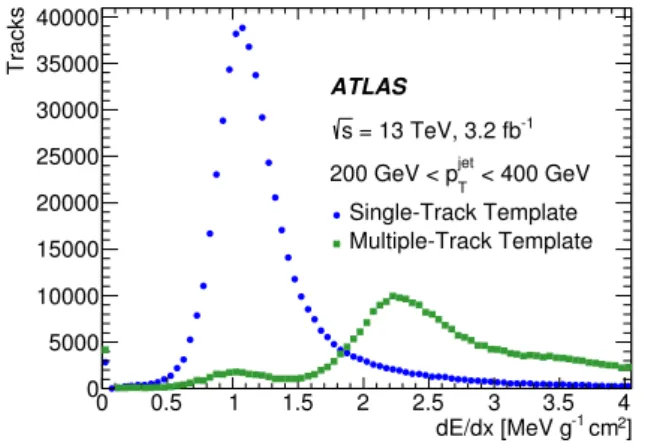
Examples of the resulting distributions are shown in Figure15. The single-track template, displayed as
circles in Figure15, contains a single peak at the dE/dx value expected for a MIP traversing the B-layer of
the pixel detector and a long tail to higher values compatible with a Landau distribution. Contamination of merged clusters in this template is 0.3–0.5% in the simulation. The multiple-track template, displayed as squares in the same figure, instead exhibits a peak in the dE/dx range expected for two MIPs. A third,
smaller peak occurs at dE/dx > 3.2 MeVg−1cm2for clusters created by three particles. The peak in the
multiple-track template dE/dx distribution at values expected for one MIP is due to the fact that multiply
used clusters can also originate from shared clusters or clusters identified as merged which, in truth, are not merged clusters.
The measurement distribution is created from tracks inside the jet core that are reconstructed from a cluster which is neither identified as merged nor shared. No additional requirements are made on other tracks using this cluster, including whether or not they satisfy the selections outlined in Section6.1. The
resulting dE/dx distribution contains single-particle clusters with a peak at the energy of one MIP and a
long tail to high values, as well as an enhanced contribution of merged clusters from two particles. Contri-butions from clusters from more than two particles are negligible. The true two-MIP clusters are created
] 2 cm -1 dE/dx [MeV g 0 0.5 1 1.5 2 2.5 3 3.5 4 Tracks 0 5000 10000 15000 20000 25000 30000 35000 40000 ATLAS < 400 GeV jet T 200 GeV < p -1 = 13 TeV, 3.2 fb s Single-Track Template Multiple-Track Template
Figure 15: Single-track and multiple-track templates for data with a jet pTin the range 200 GeV <p
jet
T < 400 GeV.
from a pair of tracks where only one track is reconstructed. Therefore, for every reconstructed track in the measurement distribution with a merged cluster, there is one particle which is not reconstructed. Using this information, the number of tracks contributing to merged B-layer clusters from two particles (N2True) is found from the sum of the number of reconstructed particles in the multiple-track template (N2Reco) and twice the number of lost particles (NLost),
N2True= N2Reco+ 2 · NLost. (1)
The sample of ρ decays discussed in Section 5.3 is used to confirm that the multiple-track template
captures merged clusters and that the second MIP peak in the measurement sample does in fact contain merged clusters where one contributing particle is not reconstructed. Therefore, to obtain the number of
lost tracks (NLost), the measurement distribution is fit with the two templates. The fraction of merged
clusters in the measurement distribution, Fmerged, is simply calculated from the post-fit number of tracks
in the multiple-track template divided by the total number of tracks (NDataReco). Finally, the fraction of lost tracks passing through the same detector element as a reconstructed track is given by:
Flost2 = NLost N2True, (2) ≈ NLost N2Reco+ 2 · NLost , (3) where
NLost= Fmerged· NDataReco. (4)
The relation is approximate due to the assumption that the lost track of a pair of tracks has the same
properties (e.g. pT and hit content) as the reconstructed track. In simulation, this assumption can be
explicitly checked by requiring the truth particle corresponding to the lost track to also pass the analysis selections. This confirms that the deviation from the approximation results in a less than 1.5% change in Flost2.
To minimize the effect of clusters created by more than two particles, the fit was performed over the range
1.1–3.07 (1.26–3.2) MeVg−1cm2for data (simulation). Contributions from clusters from more than two
events compared to data requires an adjustment of the respective fit ranges. The ranges are chosen to have the same fraction of clusters inside the fit range with respect to all clusters in the distribution. An imperfect description of the leading edge of the measurement distribution by the single-track template would affect the fitted result. Since the area of interest lies at much higher dE/dx values, the lower edge of the fit range was chosen to avoid as much as possible the leading edge of the single-particle dE/dx peak, while retaining a large sample for the remainder of the distribution.
To study the dependence of lost tracks on jet pT, the fit is performed in seven different bins of jet pT
ranging from 200 GeV to 1600 GeV in steps of 200 GeV.
The measurement is performed both on data and simulation samples. For simulation, separate templates
are constructed for each jet-pT bin. For data, the single-track and multiple-track templates are derived
from the lowest jet-pTbin, shown in Figure15, due to the small number of events at higher jet pT. It was
verified that within the statistical uncertainty of the high-pTbins, the templates derived from the lowest
jet-pTbin have the same shape within the fitted range.
6.3 Systematic uncertainties
The resulting Fmerged exhibits a statistical uncertainty due to the finite number of entries in both the
template and the measurement distributions.
Various potential sources of systematic bias were studied and are discussed below. The relative values for
data are summarized in Table1and values for MC simulation are comparable. The measured Flost2 varies
as a function of the range in dE/dx for which the distribution is fit. This is due to the different fractions
of clusters with a dE/dx of two and three MIPs falling in the fitted range. The effect was estimated by
increasing the fit range. The fitting process was repeated for six different ranges with the upper edge
increasing in 0.2 MeVg−1cm2 increments. A symmetric uncertainty, equal to the maximum change in
Flost2, is applied to each jet-p
T bin. The start of the fitted range was chosen such that small variations
have a negligible impact on Flost2.
A systematic uncertainty considered for data is the result of fitting all data jet-pTbins with the templates
from the lowest jet-pTbin. This results in an overestimate of Flost2 increasing with jet pT. To account for
this bias, a pT-dependent multiplicative correction was determined by comparing the Flost2 values fitted
in simulation with templates from the corresponding jet-pTbin with those obtained using a template from
the lowest jet-pT bin. This correction increases from about 10% to 25% for jets with a pT ranging from
400 GeV to 600 GeV and from 1400 GeV to 1600 GeV, respectively. This correction term was applied
to data Flost2 values after completing the fitting procedure. In addition, the difference between the two
simulation Flost2 values compared for the correction factor was also included as a systematic uncertainty.
An additional check performed with a large simulated sample showed a 3% to 8% bias in Flost2 in the
studied jet-pTrange due to the fraction of tracks reconstructed from ≥ 3 particle clusters, relative to the
two-particle contribution in the multiple-track template.
To validate the method, and provide an estimate of any residual biases, a truth-based closure test was
performed using simulated samples. At low jet pT, the residual dE/dx peak at values expected from
one MIP in the multiple-track template contributes to a non-closure. Also, for all jet pT, isolated-track
reconstruction efficiency, the composition of multiple-particle clusters, including particle composition
and the calibration of dE/dx itself are all covered in this non-closure estimate. This is already covered by the systematic uncertainty determined from changing the fit range described above, but also leads to a
Jet pT[GeV] Flost2 Fit range [%] Low-pTtemp. [%] Non-closure [%] Tot. syst. [%] Stat. [%] 200–400 0.061 13 0 18 23 10 400–600 0.063 12 7 11 17 6 600–800 0.070 10 13 6 17 7 800–1000 0.064 12 18 1 22 11 1000–1200 0.067 12 21 0 24 15 1200–1400 0.080 11 16 0 19 13 1400–1600 0.093 15 16 0 22 18
Table 1: Measured Flost2, relative values of leading systematic uncertainties, and total systematic and statistical
uncertainty in the fraction of lost tracks for data in bins of jet pT.
non-closure. In the lowest jet-pT bin, a non-closure of approximately+18% is observed, corresponding
to an absolute overestimation of the true Flost2 of about 0.013, but then quickly decreases with increasing jet pT. This uncertainty is included for both simulation and data with the corresponding relative values in
Table1.
Other possible sources of uncertainty are contributions to Flost2 not originating from the density of the
environment. Such contributions could come from pile-up tracks creating merged clusters with tracks in the jets, as well as lost isolated tracks. Conservative estimates based on MC studies showed that such contributions are 2% to 6% of the total Flost2 in the studied jet-p
T range. This effect is covered by the
non-closure systematic uncertainty described above.
Uncertainties in the jet energy scale calibration and resolution have negligible impact in the analysis. Possible effects due to the binning of the dE/dx distributions were studied and found also to be insignific-ant.
6.4 Results
Figure16shows the fit result for data in two bins of jet pT. The single-track and multiple-track dE/dx
templates provide a good description of the dE/dx distribution as visible from the ratio in Figure16.
Differences between event generators, such as different hadronization models and flavour compositions,
can affect Flost2 and the overall comparison of data and MC simulation. By comparing the fit results
from simulated samples made with the Pythia 8, Sherpa and Herwig++ event generators, a generator
uncertainty was derived for simulation only. For each jet-pT bin, results from Pythia are taken as the
central value and the largest difference of Flost2 between the three generators is symmetrized and taken
as the generator uncertainty. The relative generator uncertainties in the fraction of lost tracks ranges from 4% to 37% in the different jet-pTbins.
A comparison of Flost2 as a function of jet p
T for data and simulation is shown in Figure 17. As the
jet pT increases, so does Flost2, with a similar trend observed in both data and simulation. This increase
is caused by an increasing density of charged particles, which thereby causes higher collimation of the track pair, and is not due to confusion in correctly assigning clusters to tracks. At a certain point, the two particles are so collimated that the reconstructed tracks start to overlap completely up to the radius of the
Tracks 2 10 3 10 4 10 5 10 6 10 ATLAS -1 = 13 TeV, 3.2 fb s < 400 GeV jet T 200 GeV < p 0.001(stat) ± = 0.008 merged F Data 2015 Fit Single-Track Contribution Multiple-Track Contribution ] 2 cm -1 dE/dx [MeV g 0.5 1 1.5 2 2.5 3 3.5 4 Fit/Data 0.9 1 1.1 (a) Tracks 10 2 10 3 10 4 10 ATLAS -1 = 13 TeV, 3.2 fb s < 1200 GeV jet T 1000 GeV < p 0.005(stat) ± = 0.028 merged F Data 2015 Fit Single-Track Contribution Multiple-Track Contribution ] 2 cm -1 dE/dx [MeV g 0.5 1 1.5 2 2.5 3 3.5 4 Fit/Data 0.9 1 1.1 (b)
Figure 16: Data dE/dx measurement distributions (black circles) with fit results (solid line) are shown for (a)
200 GeV < pjetT < 400 GeV and (b) 1000 GeV < pjetT < 1200 GeV. The single-track template scaled by 1 − Fmerged
is shown as the single-track contribution (dashed line) and the multiple-track template scaled by Fmerged is shown
as the multiple-track contribution (dotted line). The bottom panel in each plot shows the ratio of the fit to the data
within the fit range (1.1–3.07 MeVg−1cm2).
occurs. The cluster assignment efficiency for reconstructed tracks remains constant with increasing jet
pT, indicating no degradation of performance due to the environmental effects besides the second track.
Only because of their increasingly collimated nature, the probability of losing one of the tracks rises. This effect was confirmed in simulation for tracks selected by this analysis.
The measurements in data and MC simulation are consistent across the whole studied jet-pTrange.
[GeV] T Jet p 200 400 600 800 1000 1200 1400 1600 2 lost F 0 0.02 0.04 0.06 0.08 0.1 0.12 ATLAS -1 =13 TeV, 3.2 fb s Data 2015
Simulation (Pythia 8) Total Uncertainty Statistical Uncertainty Total Uncertainty
Figure 17: The measured fraction of lost tracks, Flost2, in the jet core (∆R(jet,trk)< 0.05) as a function of jet p
Tfor
data (black circles) and simulation (red line). Vertical solid error bars indicate statistical uncertainty, while the total uncertainty is represented by dashed error bars for data and a shaded area for simulation.
7 Conclusion
This paper presents the performance of the ATLAS track reconstruction chain with detailed studies in
ded-icated topologies, such as the cores of high-pTjets and the decays of τ-leptons, that are characterized by
charged-particle separations comparable to the inner detector’s sensor granularity. The ambiguity-solver stage of the reconstruction chain is described, including the usage of a neural-network-based approach to identify pixel clusters created by multiple charged particles. The current performance is demonstrated with simulated samples of a single particle decaying to a set of collimated charged particles. In the cores of jets, the number of IBL clusters on tracks, as well as the expected track reconstruction efficiency, is robust up to the highest investigated pTvalues.
A novel, fully data-driven technique, using the energy loss to identify clusters as originating from two charged particles is introduced to measure the fraction of charged particles, creating these clusters, that
fail to be reconstructed. The results are presented using tracks with pT above 10 GeV in the core of a
jet from 3.2 fb−1 of 13 TeV proton–proton collisions at the LHC. The measured fraction of lost tracks
as a function of jet transverse momentum was found to range from 0.061 ± 0.006(stat.) ± 0.014(syst.) to
0.093 ± 0.017(stat.) ± 0.021(syst.) as the jet pTincreases from 200 GeV to 1600 GeV. Data and simulation
are compatible for the full studied jet-pTrange. This result can be used to minimize the uncertainty in the
track reconstruction inefficiency in the cores of jets relevant for jet energy and mass calibrations as well as measurements of jet properties.
Acknowledgements
We thank CERN for the very successful operation of the LHC, as well as the support staff from our institutions without whom ATLAS could not be operated efficiently.
We acknowledge the support of ANPCyT, Argentina; YerPhI, Armenia; ARC, Australia; BMWFW and FWF, Austria; ANAS, Azerbaijan; SSTC, Belarus; CNPq and FAPESP, Brazil; NSERC, NRC and CFI, Canada; CERN; CONICYT, Chile; CAS, MOST and NSFC, China; COLCIENCIAS, Colombia; MSMT CR, MPO CR and VSC CR, Czech Republic; DNRF and DNSRC, Denmark; IN2P3-CNRS, CEA-DSM/IRFU, France; SRNSF, Georgia; BMBF, HGF, and MPG, Germany; GSRT, Greece; RGC, Hong Kong SAR, China; ISF, I-CORE and Benoziyo Center, Israel; INFN, Italy; MEXT and JSPS, Ja-pan; CNRST, Morocco; NWO, Netherlands; RCN, Norway; MNiSW and NCN, Poland; FCT, Portugal; MNE/IFA, Romania; MES of Russia and NRC KI, Russian Federation; JINR; MESTD, Serbia; MSSR, Slovakia; ARRS and MIZŠ, Slovenia; DST/NRF, South Africa; MINECO, Spain; SRC and Wallen-berg Foundation, Sweden; SERI, SNSF and Cantons of Bern and Geneva, Switzerland; MOST, Taiwan; TAEK, Turkey; STFC, United Kingdom; DOE and NSF, United States of America. In addition, indi-vidual groups and members have received support from BCKDF, the Canada Council, CANARIE, CRC, Compute Canada, FQRNT, and the Ontario Innovation Trust, Canada; EPLANET, ERC, ERDF, FP7, Horizon 2020 and Marie Skłodowska-Curie Actions, European Union; Investissements d’Avenir Labex and Idex, ANR, Région Auvergne and Fondation Partager le Savoir, France; DFG and AvH Foundation, Germany; Herakleitos, Thales and Aristeia programmes co-financed by EU-ESF and the Greek NSRF; BSF, GIF and Minerva, Israel; BRF, Norway; CERCA Programme Generalitat de Catalunya, Generalitat Valenciana, Spain; the Royal Society and Leverhulme Trust, United Kingdom.
The crucial computing support from all WLCG partners is acknowledged gratefully, in particular from CERN, the ATLAS Tier-1 facilities at TRIUMF (Canada), NDGF (Denmark, Norway, Sweden),
CC-IN2P3 (France), KIT/GridKA (Germany), INFN-CNAF (Italy), NL-T1 (Netherlands), PIC (Spain), ASGC
(Taiwan), RAL (UK) and BNL (USA), the Tier-2 facilities worldwide and large non-WLCG resource
References
[1] J. M. Butterworth, A. R. Davison, M. Rubin and G. P. Salam,
Jet substructure as a new Higgs search channel at the LHC,Phys. Rev. Lett. 100 (2008) 242001,
arXiv:0802.2470 [hep-ph].
[2] ATLAS Collaboration, The ATLAS Experiment at the CERN Large Hadron Collider,
JINST 3 (2008) S08003.
[3] ATLAS Collaboration, ATLAS Insertable B-Layer Technical Design Report, ATLAS-TDR-19,
2010, url:https://cds.cern.ch/record/1291633,
ATLAS Insertable B-Layer Technical Design Report Addendum, ATLAS-TDR-19-ADD-1, 2012,
URL:https://cds.cern.ch/record/1451888.
[4] G. Aad et al., ATLAS pixel detector electronics and sensors,JINST 3 (2008) P07007.
[5] ATLAS TRT Collaboration, E. Abat et al., The ATLAS TRT Barrel Detector,
JINST 3 (2008) P02014.
[6] D. Wicke, A New algorithm for solving tracking ambiguities,
LC-TOOL-1999-007-TESLA (1999) 219,
url:flc.desy.de/lcnotes/notes/LC-TOOL-1999-007-TESLA.ps.gz.
[7] T. Cornelissen et al., The new ATLAS track reconstruction (NEWT),
J. Phys. Conf. Ser. 119 (2008).
[8] A. Rosenfeld and J. Faltz, Sequential Operations in Digital Picture Processing,
J. ACM 13 (1966) 471.
[9] E. Belau et al., Charge collection in silicon strip detectors,Nucl. Instrum. Meth. 214 (1983) 253.
[10] R. Frühwirth, Application of Kalman Filtering to Track and Vertex Fitting,
Nucl. Instrum. Meth.A 262 (1987) 444.
[11] ATLAS Collaboration, Muon reconstruction performance of the ATLAS detector in proton–proton
collision data at √s= 13 TeV,Eur. Phys. J. C 76 (2016) 292, arXiv:1603.05598 [hep-ex].
[12] ATLAS Collaboration, Reconstruction of primary vertices at the ATLAS experiment in Run 1
proton–proton collisions at the LHC, (Submitted to Eur. Phys. J. C),
arXiv:1611.10235 [physics.ins-det].
[13] ATLAS Collaboration,
A neural network clustering algorithm for the ATLAS silicon pixel detector,
JINST 9 (2014) P09009, arXiv:1406.7690 [hep-ex].
[14] T. Sjöstrand, S. Mrenna and P. Z. Skands, A Brief Introduction to PYTHIA 8.1,
Comput. Phys. Commun. 178 (2008) 852, arXiv:0710.3820 [hep-ph].
[15] ATLAS Collaboration, ATLAS Run 1 Pythia8 tunes, ATL-PHYS-PUB-2014-021, 2014,
url:https://cds.cern.ch/record/1966419.
[16] NNPDF Collaboration, R. D. Ball et al., Parton distributions with LHC data,
Nucl. Phys. B 867 (2013) 244, arXiv:1207.1303 [hep-ph].
[17] M. Bahr et al., Herwig++ Physics and Manual,Eur. Phys. J. C 58 (2008) 639,