“Sell in May and Go Away”
Adage or Self-Fulfilling Prophecy?
António Martins dos Santos
Catolica-Lisbon School of Business and Economics Antonio.martins.santos90@gmail.com
March 11, 2013
ABSTRACT
The purpose of this paper is to explore the “Sell in May” effect, which is related to the fact that financial markets seem to provide positively significant returns from November to April and not significant or negatively significant returns from May until October. The Sell in May effect is present in 30 out of 37 indexes, using a sample of 37 country indexes from 1970 to 2011. All sectors of activity are consistently affected by this seasonal pattern, being the effect stronger in production related sectors. The effect is largely felt in high market capitalization companies and less in companies with high dividend yield, being that there is not any clear pattern regarding Price-Earnings ratio. Furthermore, a strategy developed taken into account the “Sell in May” effect outperforms the benchmark, providing higher risk-adjusted returns for an investor
Keywords: Stock markets, Halloween effect, Sell in May, Anomaly, Market efficiency, Sectors, Price-Earnings, Dividend yield.
Acknowledgements: The author would like to express his sincere gratitude to: Professor
Joni Kokkonen, the Dissertation Advisor, for the constant availability and helpful feedback; his friends from the Empirical Finance course, for the continuous discussion of ideas and support, specially to Miguel Salgado and Giulio Zanon; and to his family, for all the contribution and support.
1. Introduction
“Sell in May and go away…but remember to come back in September”.
Anonymous Author
“Sell in May and go away…” is an adage that is heard across all financial markets every year, consisting on the idea that investors should sell their equity portfolio in May, invest in the risk-free asset until October, month in which they should buy back their portfolio. Historically, in London, investors had as reference for returning to the markets the last horse race of the year, buying back at St. Leger’s day. In the U.S., the Halloween day was the chosen date to buy back the portfolio. As a result, investors can profit from the bull market that has historically taken place between November and April and avoid a bear market, usually present between May and October.
The Sell in May effect is a puzzle first documented by Bouman and Jacobsen (2002) who find evidence of the presence of the effect in all markets in their sample. Bouman and Jacobsen (2002) show that the effect tends to happen not only in developed markets but in emerging markets as well. They also measure the economic significance of such findings by forming a simple portfolio and comparing two different strategies – a buy and hold strategy with a Halloween strategy, selling in the beginning of May and buying back on the 31st
of October. Finally, they discover another puzzle related to the summer months, where returns are not significant or often negatively significant, adding magnitude to the Sell in May effect.
Although already investigated by other authors, the Sell in May effect still needs clarifications, particularly concerning the ways it reflects in stocks as well as in market indexes and in sectors, other than in the U.S. market. Bouman and Jacobsen (2002) only focused on MSCI Country Indexes.
The contribution of this paper is to show how this anomaly impacts equity markets in general, attempting to pursue a deeper approach on the subject by looking into the relation between the Sell in May effect and other relevant criteria: size, value and dividend yield.
My analysis examines whether returns are positively significant between November and April and not significant or negatively significant in the other 6 months of the year. The purpose of this paper will be to understand if the “Sell in May and go away” is just a simple adage or a self-fulfilling prophecy, which repeats itself year after year.
Firstly, I look at 5 regional indexes, in order to observe, in a global mapping, how this effect is spread all around the world. Then, I scrutinize a time-series of 37 market indexes, from January 1970 to December 2011 to check if this effect is also present on the country level, when looking at market indexes. Thirdly, the 37 market indexes are divided in 10 sectors, according to Global Industry Classification Standards (GICS), to observe and understand if there are any cross-sectional differences. This will be an important step, as it will possibly provide an enlarged rationale for the anomaly. Furthermore, this paper studies the Sell in May effect by analysing the individual stocks of S&P500 and FTSE100 to grasp if, from an individual perspective, there is any erosion when you conduct the regressions stock by stock. Finally, I present an analysis of the relation between Sell in May Effect and some equity characteristics, namely size by looking at RUSSEL 3000 bottom and top 500 stocks ranked on market capitalization from January 1974 to December 2011; value, by sorting S&P500 and EUROSTOXX50 in deciles according to Price-Earnings ratio (P/E) and lastly by dividend yield (dy) through organizing these two indexes according to this criteria.
The results, considering all datasets analysed are in favour of the existence and persistence of the Sell in May Effect and these are aligned with the results of previous studies on the anomaly, such as Bouman and Jacobsen (2002) and Jacobsen and Visaltanachoti (2010). Moreover, there is evidence that the effect is particularly strong in European markets and it is robust over time, with no evidence that the effect might be disappearing as other seasonal anomalies1. This goes against Murphy’s Law
as described by Dimson and Marsh (1999). Furthermore, there is no evidence that the January effect is responsible for such significant returns and in fact there is evidence that the January effect has already lost its power across markets, with some exceptions. When looking at size, the effect is strongly felt in larger companies, meaning that investors with a portfolio integrating higher market capitalization companies are more likely to get an high return by selling in may and going away. Regarding dividend yield, it was observed that companies with higher dividend relative to the share price are far less related to the Sell in May effect. When looking at P/E, there is no clear trend or relation with the Sell in May effect.
1 See:
McLean, R.D., Pontiff, J., 2012. Does academic research destroy stock return predictability? Working paper. Boston College Fama, E. . 1998. “Market Efficiency, Long-‐Term Returns, and Behavioral Finance,” J. Financ. Econ., 49,pp. 283-‐306.
In the final part of the paper, a portfolio formed by companies in which the Sell in May effect is most seen was constructed so the common investor can profit from the effect in equity markets. This analysis was performed using one of the world’s largest financial markets, the S&P500, which should be in theory, one of the most efficient ones globally.
Although it is assumed that the bull market starts in the month of November, a robustness check was performed to better understand when in fact this event happens more significantly. There is evidence that these six months comprised by the period of November to April are the ones, which always provide considerably higher returns and hence where the bull market seems to take place.
Several seasonal anomalies have already been documented2, such as the Monday effect, the Friday effect or the January effect. However, there are two main differences between such effects and the Sell in May. Firstly, the first ones fail on being consistent over the time, as they seem to disappear or reverse itself after its discovery. With the Sell in May effect, although early documented by O’Higgins and Downes (1990) and later by Bouman and Jacobsen (2002), the effect seems to persist. Secondly, the first anomalies addressed, although providing high absolute positive returns, turn out not to be feasible when incorporating transaction costs due to a large number of mandatory transactions, whereas the Sell in May effect only has to take into account major transaction costs twice a year, when buying and selling the stocks, which do not erode the returns over time.
The analysis is organized as follows. Section 2 presents a review on the existent literature. Section 3 describes the data and methodology used. Section 4 contains the empirical results. Section 5 compares the Sell in May strategy to a buy-and-hold strategy. Finally, Section 6 summarizes the conclusions.
2
See :
French. K., 1980. Stock returns and the weekend effect, Journal of Financial Economics 8, 59-‐69;
Gibbons, M. and P. Hess, 1981, Day of the week effects and asset returns. Journal of Business 54, 579-‐596.; Thaler, R. H. 1987. Anomalies: the January effect. Journal of Economic Perspectives, 1(1),197-‐201.
2. Literature review
October: This is one of the peculiarly dangerous months to speculate in stocks. The others are July, January, September, April, November, May, March, June, December, August and February.
Mark Twain
The Sell in May adage goes back to the 17th century and was first described by O’Higgins and Downes (1990). O’ Higgins and Downes were two top asset managers from Wall Street that report a similar strategy taking into account the market timing issues stating that “it would have you in the stock market starting
October 31 and through April 30 and out of the market for the half of the year”.
Still, they do not formally test the economic significance of their results.
Bouman and Jacobsen (2002) extend the Sell in May adage by studying what they name the Halloween Indicator, by dividing the financial year between Summer months (May to October) and Winter months (November to April), being that an investor should time the market and hold a portfolio of stocks during the winter months, sell it in May and invest in the money market for the summer period. They find the existence of the effect in 36 out of the 37 MSCI country indexes for the period from 1970 through 1998. They also look for a strategy, which provides a high-risk adjusted return when compared to the benchmark. As explanations, Bouman and Jacobsen rule out data mining, the January effect, changes in interest rates, concluding that the effect is, in part, linked with vacations.
Focusing on seasonal anomalies, cloudy days are associated with a lower aggregate stock return in New York City as presented by Saunders (1993) and more recently by Hirshleifer and Shumway (2003), who analyse 26 countries, from 1982 to 1997, showing that sunshine is strongly correlated with equity returns. However, as these weather-based strategies involve frequent trading, the transaction costs eliminate the gains.
Keim and Stambaugh (1984) also investigate a seasonal anomaly, the weekend effect in stock returns, showing that there are consistently negative Monday returns for the S&P Composite, traded stocks of firms of all sizes and over-the-counter (OTC) stocks over a period going back to 1928.
Kamstra, Kramer and Levi (2003) describe a pattern in stock returns, which is analogous to the Sell in May effect, denominated as Seasonal Affective Disorder (SAD), meaning that there is a relation between length of the days and stock returns.
The idea is again a link between stock returns and seasonality. The authors relate decreasing hours of daylight with the degree of risk aversion. Less hours of daylight lead to a greater degree of risk aversion and thus to a gradual increase in stock returns when winter months start as days begin to be longer.
Cao and Wei (2005) examine an alternative seasonal pattern in stock returns. They relate temperatures with equity returns and relate different states of mind that investors may present with different temperatures. Low temperatures are related to aggressive risk taking, whereas high temperatures can be linked either with apathy or aggression. They find that, with higher temperatures, the apathy mood seem to dominate aggression, leading to lower stock returns and that with lower temperatures, higher stock returns should be expected. They conclude that stock returns are significantly negatively related to temperature, and again are faced with a Summer-Winter dichotomy in equity returns.
Hong and Yu (2009) state that investors have “gone fishing”, and that both trading activity and stock returns are lower during the summer months. Looking at July, August and September for a sample of 51 stock markets, the authors find that equity returns are lower in the summer months than in the remainder of the year. They find that this effect is particularly stronger as you move farther away from the equator. Although pursuing a different rationale from Bouman and Jacobsen (2002), the results are aligned as they both find vacations to be related to this seasonal anomaly.
Jacobsen and Visaltanachoti (2010) conduct a study on U.S. sectors, and find that 48 out of 49 industries perform better during winter than summer, looking at equity returns from 1926-2006. Returns are statistically significant in more than two thirds of their sample and there exist large differences across sectors and industries. Jacobsen and Visaltanachoti (2010) determine that the effect is very strong in the production sectors and almost absent when looking at consumer consumption sectors. Although shedding some extra light on the matter of the “Sell in May” effect, it still remains a puzzle as neither liquidity or other well-known risk factors appear to have any explanatory power.
3. Data and Methodology
Rule No.1: Never lose Money. Rule No. 2:Never forget rule No.1
Warren Buffett
3.1. Data
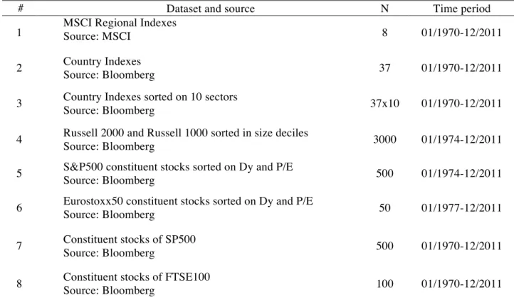
In order to better find the answer to the problem described, I am using 8 datasets that are representative of financial markets from all around the world. A summary of the datasets used is presented in Table 1, followed by a more detailed description.
Table 1 - Datasets -
# Dataset and source N Time period
1 MSCI Regional Indexes Source: MSCI 8 01/1970-12/2011
2 Country Indexes
Source: Bloomberg 37 01/1970-12/2011
3 Country Indexes sorted on 10 sectors
Source: Bloomberg 37x10 01/1970-12/2011
4 Russell 2000 and Russell 1000 sorted in size deciles
Source: Bloomberg 3000 01/1974-12/2011
5 S&P500 constituent stocks sorted on Dy and P/E
Source: Bloomberg 500 01/1974-12/2011
6 Eurostoxx50 constituent stocks sorted on Dy and P/E
Source: Bloomberg 50 01/1977-12/2011
7 Constituent stocks of SP500
Source: Bloomberg 500 01/1970-12/2011
8 Constituent stocks of FTSE100
Source: Bloomberg 100 01/1970-12/2011
The first dataset is comprised of USD denominated continuously compounded monthly returns on eight MSCI regional indexes from January 1970 to December 2011 and serves the purpose of understanding if the effect is spread worldwide and if there are exceptions. The eight regional indexes are the World Standard (Large + Mid Cap) plus the five main regions that compose the world: Europe, North America, Latin America, Asia Pacific and Middle East&Africa; plus the G7 index and the Emergent Market index. The second set of data is constituted by USD continuously compounded monthly returns on the most significant equity index of each of the 37
countries chosen worldwide3. The data length varies a lot from index to index, being
the end period of December 2011 common to all.
The third dataset is composed by the 37 country indexes grouped according to the 10 sectors GICS definition: Consumer Discretionary, Consumer Staples, Energy, Financials, Health Care, Industrials, Information Technology, Materials, Telecommunications Services and Utilities.
The fourth dataset integrates USD continuously compounded returns on the Russel3000 index. This dataset entails the bottom and upper 500 stocks sorted into market capitalization deciles with the purpose of testing for size patterns in the Sell in May effect.
The fifth and the sixth datasets are formed by the S&P500 and EUROSTOXX50 indexes sorted on P/E and dividend yield.
The final two datasets comprise the constituent stocks of two of the largest equity indexes in the world, in order to understand the impact of the Sell in May effect on a stock-by-stock level.
3.2. Methodology
The econometric methodology used in order to test the presence of the “Sell in May” effect throughout the datasets presented before is a simple regression technique that incorporates a dummy variable to discriminate the two periods under analysis. The equation is as follows (Bouman and Jacobsen, (2002)):
r! = µμ + α! S!+ ε! , (1)
,where µ is the constant in the regression and St is the dummy variable, which will
assume the value of one if month t is between November and April, and the value zero from May to October. The null hypothesis in this test is whether α1 is different
from zero. The conclusion to take is the following: if α1 is positive and significant this
rejects the null hypothesis of no “Sell in May” effect. It is a very simple approach, leading to robust conclusions while easy to analyse and allows adding more variables as well. Bearing in mind the reasoning behind this simple approach, allied to the fact that one of the criticisms regarding the Sell in May effect is that the January effect may be responsible for the Sell in May anomaly, a new equation was introduced, now taking into account the January effect. This will clarify if an investor still gets
3
significant positive returns in the “Sell in May” effect dummy (now excluding January) or if the January effect is in fact explaining all the return different from zero. The regression equation is as it follows (Bouman and Jacobsen, (2002)):
r! = µμ + α! S!!"#+ α!Jan!+ ε!, (2)
,where Jant is also a dummy variable, which will take the value of one if returns are in
January and zero in the other months. St is adjusted in order to not include January,
which will now have a value of zero. It is important to stress that the equation is based on the fact that all returns in January are due to January effect and, as expected, this strong attention will understate “Sell in May” effect and amplify the January effect. Nevertheless, it represents a test on the robustness and significance of the effect, being important to analyse if we are tackling a different anomaly than the well-known January effect.
4. Results
You only need to make one big score in finance to be a hero forever.
Merton Miller
Section 4 provides the main empirical results and is divided in eight parts. The results will be presented firstly on a broad manner by looking at regional indexes and then going for a more detailed analysis, ending on a stock-by-sock level analysis of the Sell in May effect.
In first place, results on regional division are presented. Then, are presented the results on the analysis of 37 country indexes. These are followed by the results on the sectorial analysis of the previously referred 37 market indexes, according to GICS 10 sector definition. The next set of results presents the relation between the Sell in May and size, value, dividend yield criteria. The final part of the results sections addresses the stock-by-stock analysis results.
4.1. Results on regional division
As a first step to assess the Sell in May effect from a broad perspective, table 2 follows the effect throughout the world in order to identify whether the Sell in May effect is present worldwide. The results are summarized as follows:
Considering the MSCI World Index, the Sell in May effect is positively significant in both equations and provides a positively significant Sharpe Ratio in the November-April period and a negatively significant Sharpe Ratio in the remainder of the year.
When looking at the world, firstly sorted in 5 regions, only Europe, North America and Latin America present a clear existence of the Sell in May effect. In line with the findings of Bouman and Jacobsen (2002), Europe is where the effect predominates the most and in the region of Middle East & Africa the effect is almost absent.
Finally, when contrasting two interesting, somewhat dichotomist groups, G7 and Emerging Markets, it is possible to observe that both developed and developing markets exhibit the Sell in May effect, with the returns in November-April seem to be superior to those in May-October. Regarding the Sharpe Ratio, these are positively significant for the bullish period and not significant in the bearish period.
Table 2
- Summary Results for MSCI Regional Indexes -
MSCI Indexes N α 1 αtAdj α2
Sharpe Ratio (November-April) Sharpe Ratio (May-October) World 504 1.20*** 1.29*** 0.79 0.16** -0.12* [3.10] [3.16] [1.09] [2.55] [-1.91] Europe 504 1.60*** 1.77*** 0.77 0.18*** -0.14** [3.53] [3.72] [0.91] [2.90] [-2.17] North America 504 0.97** 0.97** 0.97 0.14** -0.09 [2.42] [2.30] [1.29] [2.13] [-1.38] Latin America 288 2.43** 2.70** 1.10 0.25*** -0.03 [2.23] [2.35] [0.54] [2.91] [-0.36] Asia Pacific 288 0.87 1.13 -0.44 0.03 -0.11 [1.23] [1.52] [-0.33] [0.37] [-1.32] ME&A 108 0.59 1.41 -3.50 0.16 0.05 [0.47] [1.08] [1.51] [1.17] [0.36] G7 420 1.05** 1.23*** 0.17 0.17** -0.09 [2.50] [2.79] [0.21] [2.38] [-1.27] Emerg. Markets 288 2.25*** 2.45*** 1.29 0.26*** -0.09 [2.71] [2.80] [0.83] [3.02] [-1.02]
Notes: The t-values for the α1, α1Adj and α2, which are the parameters of the regressions that capture the Sell and May effect, adjusted and non-adjusted for the January effect are presented in brackets. Monthly Sharpe ratios were calculated using U.S. three month T-bill and their respective t-values for both the period of November-April and May-October are calculated as proposed by Lo (2002). * 10% significance; ** 5% significance; 1% significance.
4.2. Results on market indexes
In order to further answer the question if the Sell in the May effect is present in all stock markets and taking the second step in the funnel approach, it is crucial now to look at market indexes. This analysis is performed with 37 Country Indexes, as described in the data section. The conclusions are summarized in Table 3.
Looking at α1 from equation (1) described in the methodology, it is possible to
observe that 30 out of 37 indexes present superior average returns in the period of November-April when comparing to the period May-October. The strength of the effect varies across countries. Again, Europe is where the Sell in May effect becomes more evident as all countries analysed present significance. It is noteworthy to see that Nikkei in Japan and Taiwan Stock Exchange also present high significance to the Sell in May effect, going against the fact that Asia Pacific Region, as a whole, doesn’t reflect this effect.
Incorporating the January effect as a separate anomaly the Sell in May effect remains significant, although for some countries the month of January reflects a tremendous importance in the winter months, being that now 26 out of 37 country indexes present significance. These results are not presented in Table 3 in order to save space.
When looking at the Sharpe Ratios in Table 3, the Sell in May effect becomes clearer, as 32 out of 37 countries under analysis present positively significant Sharpe ratios for the November-April period and 12 out of 37 countries exhibit negatively significant SR for the remainder of the year, being that the other indexes, with the exception of 4, are not significant. Table 4 shows average SR for the two periods under analysis.
Table 3
- Summary Results on Market Indexes -
Region Market Indexes Number of
Observations α1 Sharpe Ratio (November-April) Sharpe Ratio (May-October) Asia-Pacific S&P/ASX200 235 0.77* 0.14* -0.07 HK Hang Seng 503 0.62 0.08* 0.04 Jakarta SE 344 2.30*** 0.22*** -0.04 NIKKEI225 503 1.53*** 0.11** -0.13*** Korea SE 383 1.60*** 0.14** -0.04 FTSE Malaysia 216 1.61** 0.08 -0.14* New Zealand SE 131 0.58 0.16* -0.03 Philippines SE 299 1.38* 0.14** -0.02 Singapore ST 148 0.85 0.07 -0.08 Taiwan SE 503 3.16*** 0.22*** -0.10* Thailand SE 293 1.53* 0.11 -0.06 Europe Vienna SE 234 2.19*** 0.24*** -0.17** BEL20 252 1.58*** 0.17** -0.14* OMX Copenhagen 192 1.18* 0.20** -0.04 OMX Helsinki 25 283 2.42*** 0.18*** -0.15** CAC40 293 1.98*** 0.17*** -0.16** DAX 503 1.50*** 0.14*** -0.09* Athens SE 299 1.57* 0.11* -0.04 Irish SE 347 2.28*** 0.25*** -0.11** FTSEMIB 168 2.55**** 0.12 -0.28*** AEX 347 1.88*** 0.21*** -0.10* Oslo SE OBX 191 1.96** 0.26*** -0.05 PSI20 228 1.69*** 0.16** -0.13* MICEX 171 5.43*** 0.34*** -0.10 IBEX 299 1.50*** 0.15** -0.08 OMX Stocholm 30 300 2.08*** 0.22*** -0.09 Swiss MI 281 0.87* 0.14** -0.04 Istanbul SE 100 287 2.28* 0.24*** 0.13* FTSE100 335 1.23*** 0.19*** -0.07 Middle East & Africa Amman SE 144 0.39 0.09 0.00 FTSE/JSE Africa 198 1.25* 0.26*** 0.01 North-America S&P/TSX 503 1.19*** 0.14*** -0.07 S&P500 503 0.93*** 0.13*** -0.04 Mexican SE 215 1.21 0.21*** 0.05 Latin America Buenos Aires SE 287 1.06 0.22*** 0.14** BOVESPA 264 4.16** 0.41*** 0.20*** Santiago SE 263 0.39 0.20*** 0.15**
Notes: *10% significant; **5% significant; ***1% significant. The table presents Monthly Sharpe Ratios (Lo (2002)), which were calculated using U.S. 3 month T-bill. T-statistics are not presented for space reasons.
Table 4
- Average Sharpe Ratio -
November to April May to October
Average SR 0.19*** 0.02
Naive t-stat [5.15] [-0.13]
Notes: *10% significant; **5% significant; ***1% significant. Both SR and t-stats were calculated through a simple average.
On average, from November to April, the Sharpe Ratio is positively significant, whereas for the remainder of the year it is either not significant or negatively significant, being the exception the month of July, which produces a positively significant Sharpe of 0.10. This figure is not visible in Table 4, as the values presented constitute the average of the two dichotomist periods.
The Sell in May is present all over the world equity market indexes, being the European countries the ones who produce the more robust conclusions as all European countries analysed were significant to the Sell in May effect.
4.3. Results on sectors
Answering the question if the Sell in May effect is present in all sectors of activity, the approach was to divide each of the 37 market indexes in 10 different sectors, according to the Global Industry Classification Standards: Consumer Discretionary, Consumer Staples, Energy, Industrials, Materials, Health Care, Financials, Information Technology, Telecommunications Services and Utilities. Table 5 presents the percentage of countries where the Sell in May effect is significant.in each sector. For instance, 59% of the countries in the sample show a significant Sell in May effect in the Consumer Discretionary sector.
Considering all 37 indexes, looking at α1 and α1 Adj
, it is possible to observe that 6 out of 10 sectors are statistically significant in more than half of the countries analysed, as they are over 50%. The most significant sectors in which the Sell in May effect is present are Industrial and Materials. This result is in line with Jacobsen and Visaltanachoti (2010), who find that production sectors have a stronger significance. Energy, Utilities and Health Care are the sectors with lower percentage of significance when considering the 37 indexes.
Looking at Panel 2, one can observe the results of the sectorial analysis sorted between 5 regions of the world. Again, the region which presents a stronger Sell in May effect is Europe with greater percentage overall, being that it is particularly stronger in the production-related sectors and weaker in energy, health care and
utilities. The same trends apply to Asia Pacific region, although with lower strength. The other three regions, as are formed by fewer countries, it becomes less observable on how sectors are impacted by the Sell in May effect. Nevertheless it can be stated that the effect is present not only in all regions, country indexes but also across all sectors of activity, with the production sectors showing the stronger results.
Table 5
- Summary Results on Market Indexes sorted on Sectors -
Panel 1 - 37 Indexes Panel 2 - αt Regional
GICS SECTORS αt αtAdj Asia Pacific Europe LATAM ME&A North America
Consumer Discretionary 59% 56% 45% 59% 100% 50% 100% Consumer Staples 51% 54% 45% 61% 0% 0% 67% Energy 36% 36% 9% 44% 50% 50% 100% Financials 58% 56% 36% 78% 0% 50% 67% Health Care 27% 23% 14% 31% 0% 50% 33% Industrials 71% 66% 64% 71% 100% 50% 100% Information Technology 54% 50% 63% 46% 100% 0% 100% Materials 74% 74% 60% 88% 0% 50% 100% Telecommunications 39% 39% 30% 38% 0% 100% 67% Utilities 32% 32% 38% 33% 0% 100% 0%
Notes: The table presents the percentage of countries that are significant to the Sell in May Effect in each sector. Some country indexes do not integrate all sectors of activity and so the percentage is calculated through dividing the number of significant countries in each sector, over the number of countries that integrate the sector in question. Significance is given at a 90% confidence level.
4.4. Results on deciles formed on size
In order to answer the question if the Sell in May effect varies with market capitalization of companies, that is, if size plays a role in explaining the Sell in May phenomena, I grouped the Russell 3000 bottom and upper 500 stocks into deciles according to market capitalization. The results are summarized in Table 6.
Firstly, by looking at α1, the parameter that captures the Sell in May effect in
equation (1), it is possible to note that 6 out of 10 deciles are significant for the lower market capitalization companies and 8 out of 10 deciles for the higher market capitalization companies, which may be a signal that higher market capitalization companies are more subjected to the Sell in May effect, although both presenting high percentage of significance. When incorporating the January effect, according to equation (2), the number of significant deciles goes down to 50% of significant deciles for the lower market capitalization companies, whereas for the top market capitalization companies, the number goes to 90%. Regarding Sharpe Ratio, it becomes clearer, as for the lower market capitalization, for the period of
November-April (the bullish period), all deciles present an insignificant Sharpe Ratio and for the period of May-October (bearish period) 8 out of 10 deciles are negatively significant. For the higher market capitalization companies, in the period of November-April all deciles present a positively significant Sharpe, being that for the bearish period all deciles are not significant.
Table 6
- Summary Results on Russel 3000 sorted in size deciles -
Panel 1 - Russel 3000 Lower Mkt. Cap Panel 2 - Russel 3000 Higher Mkt. Cap
Deciles αt α1Adj SR (Nov-Apr) SR (May-Oct) α1 α1Adj SR (Nov-Apr) SR (May-Oct) Low Decile 2.05** 4.46* 0.03 -0.21*** 1.55** 1.62** 0.16** -0.06 [2.33] [1.71] [0.38] [-2.81] [2.46] [2.46] [2.14] [-0.79] 2nd decile 2.61*** 4.87** 0.05 -0.27*** 1.56** 1.56** 0.22*** -0.03 [2.94] [2.33] [0.61] [-3.47] [2.38] [2.27] [2.73] [-0.36] 3rd decile 1.60** 3.19* 0.05 -0.19** 1.43*** 1.53*** 0.31*** -0.02 [2.30] [1.78] [0.65] [-2.45] [2.74] [2.80] [3.78] [-0.19] 4th decile 1.49 2.72 -0.00 -0.13* 0.84 0.93 0.17** 0.02 [1.30] [1.04] [-0.04] [-1.79] [1.54] [1.63] [2.05] [0.24] 5th decile 0.61 4.15 -0.01 -0.07 0.96* 1.13* 0.24*** 0.06 [0.61] [-0.07] [-0.06] [-0.92] [1.70] [1.91] [2.99] [-0.77] 6th decile 2.01** 3.87* 0.09 -0.19** 1.21** 1.31** 0.29*** -0.004 [2.44] [1.90] [1.12] [-2.46] [2.41] [2.49] [3.49] [-0.05] 7th decile 0.66 2.95 -0.04 -0.13* 0.92 1.01* 0.21*** 0.02 [0.87] [0.26] [-0.58] [-1.78] [1.48] [1.74] [2.64] [0.02] 8th decile 1.79** 3.26** 0.07 -0.18** 1.02** 1.19** 0.24*** 0.002 [2.51] [2.01] [0.91] [-2.52] [2.06] [2.29] [2.90] [0.02] 9th decile 1.57* 4.23 -0.00 -0.19** 1.07** 1.18** 0.33*** 0.04 [1.81] [1.16] [-0.03] [-2.46] [2.13] [2.23] [4.04] [0.49] High decile 0.93 2.99 0.03 -0.11 0.85* 0.87* 0.33*** 0.03 [1.32] [0.72] [0.35] [-1.49] [1.91] [1.88] [3.65] [0.42]
Notes: The t-values for the α1, α1Adj and α2, which are the parameters of the regressions that capture the Sell and May effect, adjusted and non-adjusted for the January effect are presented in brackets. Monthly Sharpe ratios were calculated using U.S. three month T-bill and their respective t-values for both the period of November-April and May-October are calculated as proposed by Lo (2002). * 10% significance; ** 5% significance; 1% significance.
It is possible to conclude that there is a stronger presence of the Sell in May effect when looking at the higher market capitalization stocks, though the effect is wide and present across all ranges of market capitalization. Moreover, I also found that the strength of the January effect is higher when observing lower market capitalization deciles and it is almost absent when considering higher market capitalization stocks. The results on the January effect are not included in order to save space.
4.5. Results on deciles formed on Dividend Yield ratio and Price-Earnings ratio
In order to answer the question if the Sell in May effect is related with any other criteria and to shed light on the puzzle, I sorted both S&P500 and Eurostoxx50 into d/y and P/E deciles. The results for P/E deciles and for d/y are shown in Tables 7 and 8, respectively.
Table 7
- Summary Results on Price-Earnings deciles -
Panel 1 - S&P500 Panel 2 - Eurostoxx50
Deciles αt SR (Nov-Apr) SR (May-Oct) αt SR (Nov-Apr) SR (May-Oct) Low decile 1.62*** 0.22*** -0.07 1.86* 0.13 -0.17* [2.61] [3.02] [-0.95] [1.72] [1.14] [-1.76] 2nd decile 1.32** 0.20*** -0.07 -0.07 -0.05 -0.08 [2.43] [2.68] [-0.96] [-0.07] [-0.53] [-0.85] 3rd decile 1.24** 0.23*** -0.05 3.06*** 0.30*** -0.20** [2.38] [3.08] [-0.65] [2.94] [3.10] [-2.06] 4th decile 1.31** 0.25*** -0.05 2.80** 0.09 -0.25*** [2.55] [3.43] [-0.63] [2.36] [1.01] [-2.58] 5th decile 0.85* 0.23*** 0.00 3.94*** 0.23** -0.30*** [1.92] [3.14] [-0.06] [3.64] [2.44] [-3.99] 6th decile 1.00** 0.25*** 0.00 3.34*** 0.22*** -0.17** [2.15] [3.37] [-0.04] [2.96] [2.59] [-1.99] 7th decile 1.32** 0.17** -0.06 2.15** 0.08 -0.26*** [2.21] [2.55] [0.84] [2.28] [0.89] [-2.74] 8th decile 1.41** 0.29*** 0.00 2.81*** 0.14* -0.20*** [2.48] [3.94] [-0.04] [3.09] [1.90] [-2.72] 9th decile 0.92 0.21*** 0.01 2.41** 0.13 -0.17* [1.62] [2.93] [0.20] [2.00] [1.36] [-1.78] High decile 1.54** 0.21*** -0.05 2.77*** 0.14 -0.27*** [2.35] [2.82] [-0.70] [2.90] [1.65] [-3.08]
Notes: The t-values for the α1 are presented in brackets. Monthly Sharpe ratios were calculated using U.S. three month T-bill and their respective t-values for both the period of November-April and May-October are calculated as proposed by Lo (2002). *10% significant; **5% significant; ***1% significant.
Regarding Price-Earnings ratio, based on the sample it does not seem to exist any transparent relation between the Sell in May effect and the P/E ratio. Incorporating the January effect does not add knowledge on this relation, as this effect is absent from the sample analysed. The results on the January effect are not presented in order to save space. The value factor does not add any further knowledge on the Sell in May puzzle.
Considering dividend yield, observing exclusively αt it is difficult to grasp a
S&P500, the first five deciles present significant αt, whereas only 2 out of 5 deciles
with higher dividend yield present significance, being this a first signal that higher dividend paying companies are less related with the Sell in May effect. Looking at Eurostoxx50, this is not as clear when looking at the significance of αt, as only the 9th
decile is non-significant.
Table 8
- Summary Results on Dividend Yield deciles -
Panel 1 - S&P500 Panel 2 - Eurostoxx50
Deciles αt SR (Nov-Apr) SR (May-Oct) αt SR (Nov-Apr) SR (May-Oct) Low Decile 1.94*** 0.23*** -0.07 2.59*** 0.21** -0.19** [2.72] [3.16] [-0.97] [2.61] [2.41] [-2.17] 2nd decile 1.93*** 0.28*** -0.05 2.84** 0.19** -0.16* [2.94] [3.80] [-0.65] [2.54] [2.18] [-1.89] 3rd decile 1.49*** 0.27*** -0.04 2.59*** 0.11 -0.17** [2.66] [3.67] [-0.60] [2.58] [1.54] [-2.38] 4th decile 2.20*** 0.25*** -0.09 2.61*** 0.12 -0.26*** [3.42] [3.72] [-1.32] [2.72] [1.23] [-2.70] 5th decile 1.89*** 0.23*** -0.10 4.06*** 0.26*** -0.28*** [3.45] [3.58] [-1.55] [3.52] [2.76] [-2.89] 6th decile 0.71 0.11* 0.02 1.87* 0.06 -0.18** [0.97] [1.72] [0.34] [1.84] [0.67] [-2.06] 7th decile 1.34*** 0.16** -0.09 2.82*** 0.19** -0.20** [2.60] [2.54] [-1.34] [3.06] [2.14] [-2.24] 8th decile 1.18** 0.23*** -0.04 2.79** 0.13 -0.24** [2.39] [3.08] [-0.61] [2.52] [1.37] [-2.50] 9th decile 0.68 0.16** -0.01 0.80 0.00 -0.13 [1.62] [2.37] [-0.08] [0.74] [0.00] [-1.41] High decile 0.50 0.10 -0.03 2.24** 0.14 -0.18* [1.23] [1.48] [-0.40] [2.03] [1.48] [-1.91]
Notes: The t-values for the α1 are presented in brackets. Monthly Sharpe ratios were calculated using U.S. three month T-bill and their respective t-values for both the period of November-April and May-October are calculated as proposed by Lo (2002). *10% significant; **5% significant; ***1% significant.
However, this trend can be confirmed by looking at the Sharpe Ratio. In higher d/y companies, for Eurostoxx50 only 1 out of 5 deciles present a significant Sharpe in the November-April period.
Wrapping up, the conclusions lead to the fact that earnings growth expectation measured through Price-Earnings ratio does not add any explicatory power to the Sell in May puzzle. Conversely, the Dividend yield seems to add explanatory muscles, as the companies with higher dividend yield, present in the sample, are less subjected to the Sell in May effect.
4.7 Results on individual stocks
Even if empirical evidence has shown that the principal American index is not one of the countries with the strongest “Sell in May” effect, it is not possible to forget the fact that most of the academics, investors and financial institutions see it as a symbol of the best proxy for the efficient market and thus it is assumed a better market to be tested. A summary of the results is reported in Table 9.
Table 9
- Summary Results for the S&P500 -
Index Number of Stocks "Sell in May” effect α1 only stat. significant α1 + αjan stat. significant αjan only stat. significant
S&P 500 465 (100%) 86 (18%) 74 (16%) 8 (2%) 4 (1%)
Notes: Significance is given at 95% level of confidence. Not all the S&P 500 members have been tested
due to the occurrence of different issues such as lack of data or errors in the Bloomberg library. Only 465 shares compose the final sample.
Once again, the methodology used is the same but in order to better understand how the statistics were computed, the procedure that was followed must be explained. Firstly, all the stocks were tested according to equation (1). As a result, 18% of the sample reports significant alphas. The second step was to apply equation (2) regression in order to check whether those 86 stocks that produced positive significant results represent the effective presence of the Sell in May effect or are a consequence of the amplification of the January effect. The final outcome clearly defends the preponderance of the Sell in May effect and the low presence of the January effect.
In addition, Figure 1 resumes the statistics relative to the significance of Sell in May effect through equation (1) in order to understand the relevance, if any, of the presence of the pattern described in the size deciles analysis. What it actually appears is that those results hold as they show a considerably greater concentration of positive and higher, even if not always significant at 95% level, t-stats in the upper part of the distribution.
Figure 1
- Distribution of T-statistics relative to Alphas for the S&P 500 -
The second index that has been tested is the FTSE 100. In the first part of this section, FTSE100 reported highly significant alphas, being that its undeniable relevance in the European panorama, allied to the fact that the famous adage that is being studied comes directly from United Kingdom made this choice even more intuitive. The procedure adopted is exactly the same as before and the results obtained are presented in Table 10 and Figure 2.
Table 10
- Summary Results for the FTSE100 -
Index Number of Stocks "Sell in May” effect α1 only stat. significant α1 + αjan stat. significant
αjan only stat. significant
FTSE 100 100 (100%) 14 (14%) 13 (13%) 0 (0%) 1 (1%)
Notes: significance is given at 95% level of confidence
Figure 2
- Distribution of T-statistics relative to Alphas for the FTSE00 -
Again, despite the fact that the FTSE 100 presents a very strong Sell in May effect, the percentage of positive results for the Sell in May effect for each stock is really low. Therefore, the effect seems to fade away when trying to verify it at a stock-to-stock level. However, when analysing Figure 2, apart from noticing the increased presence of high t-statistics, a closer look allows observing that
a consistent number of the stocks are on the edge between significance and the non-significance.
4.8. Robustness check
To test if the period of Sell in May effect is correctly identified, a robustness analysis was performed to determine which period has higher significance and alpha. Recalling the definition of alpha as the average monthly return of the bullish period in excess of the average monthly return of the bearish period, one would want to have the higher alpha as possible. 7 of the most important financial markets in the world were chosen for this analysis. As a result, it is possible to conclude that the months between November and April are indeed the period, where the Sell in May puzzle is more noticed. Table 11 provides some results on the different values of αt, from
Equation (1).
Table 11
αt for different periods of 6-months on Sample Country Indexes
S&P/TSX CAC40 DAX30 FTSEMIB NIKKEI225 FTSE100 S&P500
November - April 1.19*** 1.98*** 1.50*** 2.55** 1.53*** 1.23** 0.93** [2.80] [2.83] [2.89] [2.53] [3.07] [2.53] [2.29] October-March 0.75 1.32* 1.16*** 2.25** 0.97* 0.74 0.69* [1.52] [1.87] [2.22] [2.22] [1.94] [1.44] [1.70] December-May 1.12** 1.73*** 0.93* 2.13 1.53*** 1.55* 0.76* [2.18] [2.67] [1.95] [1.57] [2.82] [1.90] [1.72]
Note: The t-values for α1 are presented in brackets. *10% significant; **5% significant; ***1% significant.
Moreover, it is important to discriminate the period into smaller periods and analyse it separately to evidence which are the strongest months and understand if the period should actually be composed of this 6 months or not. The analysis will be performed with a quarterly division. In this case, the regression applied will differ, as now there is the need to add two dummy variables to explain all periods, meaning µμ will represent a quarter and the other 3 dummy variables the remaining ones. The new equation will be as follows:
r! = µμ + α!S!"+ α!S!"+ α!S!"+ ε! (3)
Once more, the conclusion is that the months between November and April are the ones that represent at maximum extent the Sell in May effect, meaning were
α1 is higher and significantly different from zero. These conclusions are presented in
Table 12
Parameters values for Quarter analysis of sample Country Indexes
Oct-Dec Jan-Mar Apr-Jun Jul-Sep Nov-Jan Feb-Apr May-Jul Aug-Oct
S&P/TSX 0.95** 0.02 -0.47 -1.10 2.02*** 1.29** 1.17* -0.56 [2.22] [0.03] [-0.77] [-1.83] [3.39] [2.16] [1.95] [-1.33] CAC40 0.84 0.76 -0.44 -1.32 1.72*** 2.42*** -0.06 -0.43 [1.51] [0.98] [-0.57] [-1.69] [2.22] [3.12] [-0.08] [-0.79] DAX30 1.22** -0.37 -0.82 -2.17*** 1.84*** 2.02*** 0.76 -0.77 [2.54] [-0.53] [-1.2] [-3.18] [2.70] [2.96] [1.11] [-1.6] FTSEMIB 0.40 2.17** -0.69 -0.88 2.55*** 2.32** -0.17 -0.62 [0.63] [2.41] [-0.76] [-0.98] [2.84] [2.58] [-0.19] [-0.98] NIKKEI225 0.08 0.80 0.48 -0.87 1.80*** 2.10*** 0.95 -1.03** [0.16] [1.18] [0.71] [-1.29] [2.69] [3.13] [1.41] [-2.18] FTSE100 0.82 0.47 -0.38 -0.91 1.67** 1.74** -0.05 -0.22 [1.66] [0.68] [-0.54] [-1.29] [2.4] [2.51] [-0.07] [-0.45] S&P500 1.07** -0.49 -0.23 -1.46** 1.37** 0.91 0.60 -0.19 [2.52] [-0.81] [-0.38] [-2.43] [2.29] [1.52] [1.00] [-0.46]
Note: The t-valuesare presented in brackets. *10% significant; **5% significant; ***1% significant.
One can clearly understand that both quarters starting on November and February are positive and significant for all indexes considered, leading to the conclusion that the six months of November to April constitute indeed the period where Sell in May effect is most felt.
5. Strategy on Sell in May effect
“If you must play, decide on three things at the start: the rules of the game, the stakes and the quitting time.”
Chinese Proverb
When talking about academic research on anomalies, any sort of discovery is meaningless if not conducive to provide consistent returns. For this reason, the final step of this paper is focused on finding a strategy based on the Sell in May effect that is able to beat the benchmark.
The approach is as follows: firstly, all the stocks from the S&P 500 that presented significant alphas in the final part of section 4 were collected. However, in order to have a time span that is wide enough for computing the strategy, only the ones that were exhibited at least 30 years of data were considered. Integrating this constraint, the final number of stocks is 49 which will compose an equal-weighted portfolio as it generally outperforms other sophisticated asset allocation models as argued by DeMiguel, Garlappi, and Uppal (2009).
Following this approach, two strategies are designed: “Buy & Hold” for all the period of estimation and another called Sell in May, where instead of keeping constantly the position throughout the year, the investor should divest from the market and go for the risk free asset – a 3-month US T-bill – during the bearish period of the markets (May-October) buying back all his position on the Halloween day4
.
Finally, the statistics are computed for simply holding the market portfolio (S&P500) and the excess returns of the portfolios – holding all the stocks throughout the year and Sell in May – are tested out-of-sample for the two different strategies, using the “rolling-sample”5
approach described in DeMiguel et al. (2009). Table 13 summarizes the results, presenting annualized excess returns, standard deviation, Sharpe ratio and certainty equivalent6.
Looking at Table 13, the results obtained are self-explanatory, as the returns of the Sell in May strategy are outperforming the market by a substantial margin with the important feature that, as expected by construction, given the investment in risk free during bearish times, the strategy provides lower standard deviation. Moreover, when considering Sharpe ratios, the only significant and positive is the Sell in May portfolio strategy exceeding around four times the other two. It is important to state that each Sharpe Ratio was adjusted due to high serial-correlation7
on the returns. In addition, the Certainty Equivalent is also the highest one, showing how remarkable this strategy can be for an investor.
4
For simplicity, any kind of transaction cost will not be initially taken into account.
5
Initial estimation period of 2 years. Rolling rebound each month.
6 Calculated through R – (
γ/2)σ , assuming γ = 4
7
Suggested on Lo, A. “The Statistics of Sharpe Ratio”. Financial Analysts Journal, 58 (2002), pp.36-‐50
Table 13
- Comparison between strategies Out-of-sample -
Strategy Excess Returns Standard Dev Skewness Excess Kurtosis Sharpe Ratio Certainty Equivalent
S&P 500 2.44 15.77% -0.90 3.09 0.15 2.51% [0.87] [0.84] Buy &Hold 2.60% 20.46% -3.43 15.60 0.09 -5.77% [0.70] [0.51] Sell in May 7.60%*** 11.85% 0.22 -1.55 0.39** 4.79% [3.51] [2.04]
Notes: All the statistics are annualized averages of monthly data. The values reported in brackets are t-stats. Sharpe Ratio
is computed using U.S. 3 month T-bill and their respective t-values for both the period of November-April and May-October are calculated as proposed by Lo (2002). *10% significant; **5% significant; ***1% significant.
Furthermore, skewness and kurtosis should be subject of discussion and comparison as well. Sell in May strategy once more seems to outperforms both other strategies as it can provide fatter right tails and returns with higher concentration around the mean, avoiding thus potential huge losses – which is not the case when we look to high positive excess kurtosis of both buy & hold strategy and the market.
5.1. Incorporating transaction costs
Although this strategy seems to clearly outperform both the market and a buy & hold strategy of the stocks portfolio, one should take into account the transaction costs associated with such strategy. A break-even analysis was performed in order to determine at what point, integrating transaction fees, the excess return of Sell in May strategy becomes inferior to the buy & hold strategy
The analysis performed takes into consideration the monthly rebalancing that is necessary for the implementation of the equal-weighted portfolio. As a result, both strategies, Sell in May and buy & hold, have transaction costs, although one should anticipate an higher impact in the Sell in May strategy as the investor has the need to buy and sell all the portfolio each year. Besides, the approach taken is pretty straightforward. The adjustments on the weights, meaning buying or selling the specific stock, will be dependent on the stock’s return and how it impacts the stock’s weight to increase or decrease. The necessary adjustment would be the difference between this new weight and the fixed weight – 1 over N, so 2.04%. Thus, in Table 14 are presented the corresponding costs, as a percentage of the initial investment, for each strategy consistent to different values of commissions to be charged over a single transaction.
Table 14
- Transaction Costs as a % of Initial Investment given a commission for a single transaction -
0.50% 1.00% 1.50% 2.00% 2.50% 3.00% 3.50% 4.00% 4.50% 5.00%
“Sell in May” 1.11% 2.21% 3.32% 4.42% 5.53% 6.63% 7.74% 8.84% 9.95% 11.05%
Buy & Hold 0.30% 0.59% 0.89% 1.18% 1.48% 1.77% 2.07% 2.36% 2.66% 2.95%
The “Sell in May” Strategy clearly has higher cost to the investor than a buy & hold Strategy and its growth curve is significantly different.
Additionally, in Figure 3, it is possible to observe the behaviour of the transaction costs on the Sell in May strategy, meaning that as transaction fees go
higher, higher would be the cost of the portfolio as a percentage of the initial investment.
Figure 3
- Equalization fee for “Sell in May” strategy -
The break-even point, where the gains from the strategy are completely wiped out due to transaction costs, is the intersection of both curves, which produces an approximately fee commission of 3,1%. Consequently, any fee commission charged to an investor that it is below this figure would allow him to profit by applying the Sell in May strategy.
VI. Conclusions
“Only when the tide goes out do you discover who’s been swimming naked”
Warren Buffett
Several centuries later, the ancient English adage “Sell in May and go away” still seems to affect the course of the equity markets and assumes itself as self-fulfilling prophecy. Can the rationale for the effect only lie on the accumulation of different kinds of common events that occur during the November-April period, such as the end of the fiscal year, the so called January effect, payments of dividend or closing of the accounting year for most of the companies? It may be also related to volume or liquidity. Academics still do not find consensus and reasoning and that is why this effect still remains a puzzle. There is, in fact, empirical evidence of a bull market between November and April and a bear market, present between May and September. That was the main hypothesis this paper attempted to answer, and not to provide the absolute reasons why it is so.
0% 4% 8% 12% 0,50% 1,00% 1,50% 2,00% 2,50% 3,00% 3,50% 4,00% 4,50% 5,00% A n n u al C os t as % of I n ve stme n t Transaction fee
Moreover, the evidence that higher and positive returns occur between November and April is strong, tested for any kind of robustness and persistent over time as 14 more years of data and different periods of market turmoil have been added since Bouman and Jacobsen (2002) documented the effect.
The Sell in May effect has a higher preponderance in European countries, though being its presence is undeniable all over the world. Also, the deciles analysis of Russel3000 led to the conclusion that companies with relatively higher market capitalization are more affected. Moreover, when tested on single stocks, the Sell in May effect appears to slightly vanish. Additionally, the Sell in May effect is almost absent when confronted with higher dividend yield companies and there is no clear pattern when Price-Earnings ratio enters the equation.
A simple strategy based on the Sell in May effect outperforms the benchmark providing interesting and rewarding results for an investor. This outperformance is possible with a strategy that is less risky than simply holding the market index, measured by standard deviation, skewness or kurtosis.
References
Bouman, S., Jacobsen, B., 2002, ”The Halloween Indicator, "Sell in May and Go Away": Another Puzzle”. The American Economic Review, Vol. 92, No. 5, 1618-1635.
Cao, M., Wei, J., 2005. Stock market returns: A note on temperature anomaly, Journal of Banking and Finance 29, 1559-1573.
DeMiguel, V, Garlappi, L., Uppal, R., 2009, “Optimal versus naive diversification: How inefficient is the 1/N portfolio strategy?” Review of Financial Studies, 22, 1915-1953.
Fama, E., 1965, "The Behavior of Stock Market Prices". Journal of Business, 38, 34– 105
French. K., 1980. Stock returns and the weekend effect, Journal of Financial Economics 8, 59-69
Gibbons, M., Hess, P., 1981, Day of the week effects and asset returns. Journal of Business 54, 579-596.
Hirshleifer, D., and T. Shumway, 2000, Good day sunshine: Stock returns and the weather, Journal of Finance, 58, 1009–1032.
Hong, H., J. Yu, forthcoming 2009. Gone fishin’: Seasonality in trading activity and asset Prices, Journal of Financial Markets.
Jacobsen, B., Abdullah M., Visaltanachoti, N., 2005, Seasonal, size and value anomalies, Working Paper, Available at SSRN: http://ssrn.com/abstract=784186 Jacobsen, B., Marquering, W.A., 2008. Is it the weather? Journal of Banking and Finance, 32, 526-540
Jacobsen, B., Visaltanachoti, N., 2006, “The Halloween Effect in US Sectors,”, Financial Review, 44, 437-459.
Kamstra, M.J., Kramer, L.A., Levi, M.D., 2003. Winter blues: A SAD stock market cycle, American Economic Review 93, 324-343.
Keim, D. B.,1983 , Size-Related Anomalies and Stock Return Seasonality: Further Empirical Evidence. Journal of Financial Economics, 12, 13-32.
Lo, A., 2002, The Statistics of Sharpe Ratios, Financial Analysts Journal 58, 36-50. Lucey, B. M., & Zhao, S. 2008. Halloween or January? Yet Another Puzzle. International Review of Financial Analysis, 17, 1055–1069
McLean, R.D., Pontiff, J., 2012. Does academic research destroy stock return predictability? Unpublished working paper. Boston College.
O’Higgins, M., Downes, J., 1990, “Beating the Dow, a high-return-low-risk method for investing in industrial stocks with as little as $5000”. Harper Collins, New York Saunders, E. M. J., 1993, Stock prices and Wall Street Weather, American Economic Review 83, 1337-1345.
Thaler, R. H. 1987. Anomalies: the January effect. Journal of Economic Perspectives, 1, 197-201.
Appendix
Appendix I – Detailed Presentation of Country Indexes
Region Market Indexes Number of
Observations Countries Bloomberg Ticker
Asia-Pacific
S&P/ASX200 235 Australia AS51
HK Hang Seng 503 Hong Kong HSI
Jakarta SE 344 Indonesia JCI
NIKKEI225 503 Japan NKY
Korea SE 383 South Korea KOSPI
FTSE Malaysia 216 Malaysia KLCIADV
New Zealand SE 131 New Zealand NZSE50FG
Philippines SE 299 Philippines PCOMP
Singapore ST 148 Singapore FSSTI
Taiwan SE 503 Taiwan TWSE
Thailand SE 293 Thailand SET
Europe
Vienna SE 234 Austria WBI
BEL20 252 Belgium BEL20
OMX Copenhagen 192 Denmark KAX
OMX Helsinki 25 283 Finland HEX25
CAC40 293 France CAC
DAX 503 Germany DAX
Athens SE 299 Greece ASE
Irish SE 347 Ireland ISEQ
FTSEMIB 168 Italy FTSEMIB
AEX 347 Netherlands AEX
Oslo SE OBX 191 Norway OBX
PSI20 228 Portugal PSI20
MICEX 171 Russia CF
IBEX 299 Spain IBEX
OMX Stocholm 30 300 Sweden OMX
Swiss MI 281 Switzerland SMI
Istanbul SE 100 287 Turkey XU100
FTSE100 335 U.K. UKX
Middle East & Africa
Amman SE 144 Jordan JOSMGNFF
FTSE/JSE Africa 198 South Africa JALSH
North-America
S&P/TSX 503 Canada SPTSX
S&P500 503 U.S.A. SPX
Mexican SE 215 Mexico MEXBOL
Latin America
Buenos Aires SE 287 Argentina MERVAL
BOVESPA 264 Brazil IBOV