A Work Project, presented as part of the requirements for the Award of a Master’s
Degree in Economics from the NOVA – School of Business and Economics
The effect of serial correlation in time-aggregation of
annual Sharpe ratios from monthly data
Pedro Miguel Carregueiro Jordão Alves
Student no. 3080
A project carried on the Master’s in Economics Program under the supervision
of:
Professor André Castro e Silva
Abstract
The Sharpe ratio is one of the most widely used measures of risk-adjusted returns. It
rests on the estimation of the mean and standard deviation of returns, which is subject to
estimation errors. Moreover, it assumes identically and independently distributed returns,
normality and no serial correlation, which are very restrictive assumptions in general. By using
the Generalized Method of Moments approach to estimate these quantities, the assumptions
may be relaxed and a more efficient estimator can be derived, by allowing serial correlation in
returns. The purpose of this research is to show how serial correlation can affect the
time-aggregation of Sharpe ratios, changing the ordering of a ranking of assets based on the ratio.
Introduction
Assessing the performance of an asset or investment fund is not readily done through
simply looking at the returns generated. If an asset has higher returns than another, does that
mean it is necessarily a better investment? Or is that excess return relative to the other asset
generated by some intrinsic characteristic of the asset? If the two previous questions are
considered, one would easily conclude that returns alone are not enough to assess performance
and that some other characteristic(s) of the asset should be taken into account, namely, some
measure of how those returns could change over time (return variability). This, in general, is
captured by using a proxy for the risk inherent to the specific asset. In short, there was the need
for a measure that adjusted returns to the characteristics of the asset, defined to be its “risk”.
The Sharpe Ratio, which is one of the most widely used measures of risk-adjusted
returns, does exactly that. By dividing excess returns (over a benchmark, usually the risk-free
asset) by its standard deviation, used as a proxy for total risk of the asset, one can get a
comparable measure of the performance of the asset, adjusted to its specific characteristics. In
sense, an asset or fund that generates more excess returns for the same level of risk, would yield
a higher Sharpe ratio and, thus, be a better investment.
The ratio can be used in two different contexts, either to provide an assessment of what
the contribution of a specific asset to a portfolio’s returns would be, for example, or to measure
past performance of funds, managers or assets. In the first case, one would choose a model for
expected returns to forecast what returns are expected to be in the future, estimate the ex-ante
Sharpe ratio, use it to order the assets under consideration and decide which would be valuable
additions to a portfolio. In the second case, by looking at realized returns to estimate the ratio
one can get a sense of the past performance of some fund, fund manager or asset. Thus, we can
have two different approaches to estimating the ratio, one that is forward looking (ex ante) and
the other backward looking (ex post).
From this brief introduction, it can easily be inferred that there are some problems
inherent to this method of assessing risk adjusted returns. Firstly, there are problems regarding
the assumptions one makes when estimating the ratio, such as normality in returns, identically
and independently distributed returns and no serial correlation, which are not verified generally.
In addition, in the case of ex ante Sharpe ratio, which model of expected returns to use?
Moreover, when estimating the ratio, it is common to use data with a shorter frequency,
such as monthly data, and then aggregate the result into annual values. If the assumptions
mentioned above are verified, the standard scaling method can be used. However, if the
assumptions are violated, the scaling factor is also subject to change. This is especially pressing
in the presence of serial correlation, which might underestimate or overestimate the aggregated
value.
The accuracy of the estimation of the Sharpe ratio is dependent on its statistical
properties, which can vary greatly among funds/assets, depending on their investment
highly volatile, than if volatility is low. This way, the estimation of the ratio must be computed
and interpreted depending on the specific characteristics of the investment fund’s style which
have generated the returns. Serial correlation, especially, can affect the estimation of the ratio
by deviating the distribution of returns from the normal distribution. In particular, should one
want to aggregate a monthly Sharpe ratio to an annual value, by using the multiplier that
accounts for serial correlation, one would get a smaller value compared to the standard
approach, in the presence of positive serial correlation, and larger value if there is negative
serial correlation.
The purpose of this research is to show the impact of serial correlation in
time-aggreation, in the context of the ex post measure, derive the estimators of the ratio under less
restrictive assumptions by using the generalized method of moments approach, pioneered by
Lars Peter Hansen (1982), and show how the values obtained under the different assumptions
might change. It adds to the existing literature by building on Andrew Lo’s (2002) work,
extending the scope of his research to stocks, in addition to mutual funds, and using a
considerably larger dataset.
The empirical study is performed over a dataset of time-series of 4560 mutual funds and
6475stocks, with more than 5 years of monthly data each.
Results suggest that the method used to compute the ratio indeed plays an important role
when performing time aggregation, with the ordered ranking changing depending on the
method.
Literature Review
Being one of the most widely used methods of computing risk-adjusted returns, the
Sharpe ratio has been the object of extensive study in the literature. This literature ranges from
each asset. It also relates to the work on which Finance is built, since it rests on the basic notion
that one needs to consider both risk and return when evaluating financial alternatives.
In his seminal paper “Portfolio Selection”, Henry Markowitz (1952) developed a
framework with which to compare portfolios of securities, supported by the concept that any
rule of investment should imply the superiority of diversification, otherwise it must be rejected.
The author considers the case when an investor maximises the value of (discounted) expected
returns, rejecting it due to the fact that investors following this rule would allocate all the funds
to the security with the greatest discounted value and never to a diversified portfolio. Markowitz
then shows that if the investor faces a trade-off between the expected return of a portfolio and
its variance, the expected return-variance rule, then it would imply diversification. Using this
rule, a mathematical framework for the analysis of securities was derived, which related the
expected return of a security, measured by the mean of expected returns, to its variance (or
standard deviation), the latter being a proxy for risk (volatility). According to this framework,
an investor choosing among efficient portfolios would be able to get higher expected returns
only by taking in more risk. Additionally, it implied that diversification would occur not by
means of selecting a large number of securities alone, but only if those securities did not have
high covariance among themselves. This insight, further developed in Markowitz (1959), laid
the foundations for portfolio theory, which is the basis upon which more recent portfolio
management analysis and tools were built. The choice was now between high return but riskier
investments or low risk, low return investments, and the investor could “pay” with a bit more
risk to get higher returns, according to the individual risk aversion.
Later, building on Markowitz work, Sharpe (1963, 1964) and Lintner (1965) proposed
the joint analysis of all assets included in a portfolio to determine the risk and return of the
whole portfolio. The authors developed a general equilibrium model, the capital-asset pricing
the total portfolio risk. This contribution, denominated Beta, became a basic indicator of
financial decisions. Because Beta equals the covariance of the asset with the market, divided
by the variance of the market, it provides us with a measure of how sensitive the asset is to
movements in the market, and is, thus, another proxy for risk. Jack Treynor had developed a
similar framework before Sharpe and Lintner, in Treynor (1961, 1962), but the articles were
not published at the time and, thus, the author was not credited with the creation of the CAPM.
With a proper framework with which to evaluate assets and portfolios, questions
regarding performance of assets or funds began to arise. The problem became which proxy for
risk to use, in the case of performance evaluation.
Several measures were proposed, such as the Treynor ratio. This ratio is computed by
dividing excess returns by Beta, which represents the systematic risk of the asset. It rests on the
premise that diversification will not remove the risk inherent to the whole market and, thus, it
must be penalized. This ratio is backward-looking in its nature, which presented a limitation –
assets or portfolios with a Beta equal to 1.5 in the past, for example, will most likely not have
that value for Beta indefinitely. Moreover, it is a ranking criterion which is only useful if the
ordered portfolios are part of a larger, fully diversified portfolio, otherwise, portfolios that have
similar systematic risk, but varying total risk, will be ranked the same.
Sharpe’s (1966) seminal paper “Mutual Fund Performance” advances another
alternative to measure risk-adjusted returns. The author builds on Treynor’s work that
suggested a predictor of mutual fund performance, which incorporated the volatility of a fund’s
return when assessing its performance, proxied by the above-mentioned Beta. Sharpe tests the
empirical measure derived by Treynor to evaluate its predictive power and suggests a different
measure for comparison, which he named reward-to-variability ratio (R/V). The author argues
that ex post performance of mutual funds could vary based on two aspects: funds could exhibit
or by wrongly predicting the risk of particular portfolios, or funds that hold portfolios with
similar variability could exhibit significant differences in average returns because of managers’
inability to pick incorrectly priced securities and/or by not properly diversifying their portfolios.
Sharpe argues that since proper mutual fund management would require selection of
incorrectly priced securities, effective diversification and the selection of a portfolio in the
desired risk class there is room for differences in the performance of different funds.
The author claims that the results obtained by R/V show differences in performance can
be imperfectly predicted – though not indicating the sources of the differences – and that there
is no assurance that past performance is the best predictor of future performance. Additionally,
Sharpe shows the Treynor ratio holds more predictive power than R/V, provided there is a
reasonable assurance that the portfolio is properly diversified.
Moreover, the fact that past performance might provide some predictive power for
future performance, as measured by the Treynor ratio, does not imply that differences in
performance arise due to differences in managerial skills. In fact, the author shows that the high
correlation among mutual funds’ returns suggests the diversification is being properly achieved
by most and, thus, differences in performance might arise due to inability of picking incorrectly
priced securities or differences in expense ratios – if the market is efficient, funds that spend
less in research should show the best (net) performance, otherwise, if it is not efficient, funds
that spent more may gain enough to offset the increased expenditure and exhibit better net
performance.
In 1994, William F. Sharpe (1994) systematized the Sharpe ratio by providing a
comparison between it and other alternatives measures, generalizing the concept and
demonstrating the broad range of possible applications. This was motivated due to the
widespread use and modifications that the R/V ratio, initially proposed, suffered over the years,
estimators and argues for its time dependence, given that it assumes no serial correlation.
Additionally, Sharpe demonstrates how the Sharpe ratio, multiplied by the square root of the
number of observations, would equal a t-statistic for measuring the significance of the mean
differential return. Finally, because it does not take correlations between assets into account,
such information must be incorporated when making decisions that may affect important
correlations in the portfolio.
The Sharpe ratio, as it is proposed, assumes that the distribution of returns follows a
normal distribution, that returns are identically and independently distributed and that there is
no serial correlation. The literature developed in the meantime has shown that these are not
realistic assumptions in most cases and, thus, there have been several proposals to deal with
these shortcomings. Several modifications to the Sharpe ratio and different ratios have been
proposed.
Still on the subject of mutual fund performance, the work by Kothari and Warner (2001)
uses simulated funds in which abnormal returns are introduced and studies their performance
using regression based models, namely, the Sharpe-Lintner Capital Asset Pricing model,
Fama-French 3-Factor model and Carhart 4-factor model. The CAPM and Jensen’s Alpha measure
were introduced for power comparison between the measures and because of their popularity.
The authors report two main results: performance measures used in mutual funds’ research
typically do not detect large abnormal returns if the funds’ characteristics differ from that of a
value-weighted market portfolio; and standard event-study procedures can greatly improve the
evaluation of performance. Related to this research is Daniel et al. (1997) which suggests that
characteristic-based measures reduce the standard errors of abnormal performance measures.
Smith and Tito (1969)provide an overview of 3 ex post measures of fund performance,
the Sharpe ratio, Treynor Ratio and Jensen’s alpha (referred by the authors as Sharpe
how risk can be introduced in performance measures and how the measures relate to each other.
The authors conclude there is little difference in the measures when used to rank a series of
funds based on ex post performance, but when comparing to the market, conclusions are not as
direct, with statistical problems arising and critical assumptions having to be made in order to
perform market comparisons. It was shown that Treynor Volatility provided a more favourable
view of performance than the Sharpe Variability, with funds beating the market more frequently
than if measured by Sharpe. Moreover, the authors suggest the use of a modified Jensen
measure, which is based on a preferable estimating equation and does not exclude the slope
(volatility) coefficient which would introduce bias in the analysis. In addition to comparing the
different performance measures, this study added to the literature on market efficiency, stating
that mutual funds are not able to beat the market, on average, suggesting the abnormal returns
could have been obtained due to sheer luck.
In addition to the Treynor and Sharpe ratios, several proposals of different ratios were
made, such as Sortino’s ratio which is similar to Sharpe’s but scales the excess returns by the
standard deviation of negative returns, instead of volatility of returns.
Dowd(1999)also provides an approach to estimating the ratio such that it adjusts it for
risk, both as an ex ante and ex post measure. The author does so by comparing how the inclusion
of an individual asset would influence the ratio, computing the minimum excess return that
asset would have to provide to the portfolio to increase the Sharpe ratio.
Another approach that was developed by Israelsen (2005) makes use of the absolute
value of the mean excess returns as an exponent of the sample standard deviation in the
denominator.
Scholz (2007) provides an overview of the related modifications to the Sharpe ratio.
Other examples of literature on mutual fund performance would be Elton, Gruber and
performance and not on the biases implied by each method. It is shown that because mutual
funds that disappear, usually do so due to poor performance, studying only funds that survived
would overstate the results. Additionally, the authors show that failing to eliminate survivorship
bias would lead the researcher to spurious conclusions about the role of the fund’s
characteristics on return.
Additionally, some authors show that the Sharpe ratio can easily be manipulated by
hedge funds. These funds can manipulate the ratio through covered call writing that introduces
non-linear returns, for example, which in turn influences the tails of the Sharpe ratio’s
distribution and thus, its estimator, as shown by Leland (1999), Lhabitant (2000) and
Goetzmann et al. (2002, 2007).
Moreover, Harding (2002) suggests that by eliminating the highest returns of a
time-series can increase the Sharpe ratio. It is shown that under mild conditions a high positive excess
return in a prospective period might not necessarily increase the ratio.
Christie (2007) argues that the Sharpe ratio is inappropriate for investment fund
rankings due to the general estimation error in computing the sample statistics. Moreover,
Miller and Gehr (1978) find the exact bias in the ratio’s estimator, which does not affect the
ranking of funds with equal time lengths but overestimates the absolute value of the computed
ratio.
A different strand of the literature focused on the statistical properties of the ratio, in
particular, the properties of returns, in order to estimate it taking them into account, rather than
trying to modify the ratio itself.
Bao and Ullah (2006) and Bao (2009) present estimators that were derived assuming
returns are not IID, showing that the bias and variance formulae depend upon the structure of
covariance of the data generating process. By using an AR(1) model the effects of the series
inclusion of higher moments, such as skewness and kurtosis, when estimating the ratio. By
including higher moments one can better describe and take into account in the estimation the
real distribution of returns, rather than by assuming said distribution follows a normal.
Following the literature on the statistical properties of returns, there is empirical
evidence that portfolio returns are not normally distributed. Fama (1965) shows that returns
distributions have in general longer tails than the normal distribution, in line with the previous
Mandelbrot hypothesis that price changes conform better to stable Paretian distributions with
exponents less than 2, than a normal. Moreover, and in contrast to what has been stated before,
the author found no evidence of dependence in the data, arguing in favour of the random walk
hypothesis and the assumption that returns are independent.
Schumacher and Elling (2011) found out that, under certain conditions, neither
asymmetry nor fat tails make the using of the Sharpe ratio inappropriate.
Chae and Lee (2017) argue that higher distribution uncertainty leads, in general, to
higher returns, by measuring the difference between the distribution of an individual stock
return and the distribution of the market return.
Kacperczyk and Damien (2011) propose using a Bayesian semiparametric approach to
incorporate uncertainty about the type of the distribution of returns. The authors show that
distribution uncertainty is highly time-varying. Moreover, it is argued that distribution
uncertainty implies investors allocate less money to to risky assets, relative to investors facing
parameter uncertainty.
Ho (2006) suggests the use of a long-memory stochastic volatility model (LMSV), as
opposed to short-memory autoregressive processes, to estimate the ratio. The author shows that
using LMSV only the estimation error of the standard deviation contributes to the limit
distribution, contrary to the short-memory volatility model, where both estimation errors are
Boynton and Chen (2017) develop a parametric bootstrap approach to estimate the
predictive Sharpe ratio – it yields the value of the ratio that is most likely to be faced by the
investor, out-of-sample. It presents an advantage relative to the common Sharpe ratio in that it
incorporates distortions from estimation errors. Compared to the normal approach, the
bootstrap approach developed by the authors provides better out-of-sample predictability. It
allows the investor to test a specific data set and find the model that best fits that data, which is
advantage given that there is no model that fits the data best in all circumstances.
Woehrmann, Semmler and Lettau (2005) study the time-varying characteristics of asset
prices, trying to show whether the dynamic stochastic growth model is able to replicate time
variation in said characteristics, in particular in the Sharpe ratio. It is argued that the standard
intertemporal asset pricing theory does not explain successfully the (unconditional) first
moments of asset market characteristics, such as the Sharpe ratio. The authors follow the Local
Linear Maps technique (LLMs) of Ritter, Martinetz and Schulten (1992) to approximate
conditional expectations in the Euler equation, so as to numerically solve the underlying
intertemporal economic model while allowing for non-parametric expectations in the
expectations approach. The time-varying Sharpe ratio is obtained following Hardle and
Tsybakov (1992) by estimating a nonparametric univariate stochastic volatility model, where
conditional mean and variance of excess returns are unknown functions of past returns. The
authors found evidence the standard dynamic stochastic growth model is able to capture
countercyclical movements of the Sharpe ratio over the business cycle. Moreover, it is shown
that this estimation by Monte Carlo simulations dominates the standard GMM approach for
small samples.
Aftab, Jungwirth, Sedliacik and Virk (2008) compare the use of a GMM approach and
a maximum likelihood estimation when deriving the statistical distribution of the Sharpe ratio.
the test of normality is rejected under both approaches. Moreover, using the third and fourth
moment conditions in the GMM estimation yields minimal differences, suggesting over
identification is not advantageous.
The literature on the Sharpe ratio is very extensive and covers a broad range of subjects.
This research, motivated by Lo’s (2002) paper which pointed out that serial correlation in
returns might change the ordering of a ranking of mutual funds and hedge funds based on the
Sharpe ratio, will focus on the effect of serial correlation when computing time-aggregation of
Sharpe ratios. To show the effect of serial correlation, the author derived the distribution of the
Sharpe ratio under the initial assumptions and the distribution under less restrictive ones,
following the approach pioneered by Lars Peter Hansen in is seminal paper “Large Sample
Properties of Generalized Method of Moments Estimation” (1982). Lo shows that the approach
used to estimate returns changes the initial ordering of the funds, especially for hedge funds.
It is argued that the time-series properties of investment strategies can have non-trivial
impact on the Sharpe ratio estimator, especially when computing an annualized Sharpe ratio
from monthly data. Lo argues that the standard multiplier used is valid only under very
restrictive assumptions and that the correct scaling factor depends on the serial correlation in
returns.
In order to illustrate the potential impact of serial correlation in returns, the author
assumes returns follow a first-order autoregressive process (AR(1)). The AR(1) process
assumes that returns in period t can, to some extent, by forecasted by returns in t-1. Using this, a correct scale factor for the Sharpe ratio is derived, taking into account possible serial
correlation in returns. Additionally, Lo shows that the use of the robust Sharpe ratio estimator
and the scaling factor should not be used if there is not significant serial correlation in returns,
appears in the asymptotic variance of the GMM estimator. More details on this will be provided
in the methodology section.
An overview of the limitations and violations of the assumptions generally used in
financial literature, such as violations of IIDness in returns or normality, problems in time
aggregation, tests of several models for stock prices and returns, among other issues, can be
found in Lo and MacKinlay (1999).
Finally, the use of the GMM procedure is motivated by the fact that, unlike maximum
likelihood estimation (MLE), it does not require complete knowledge of the distribution of the
data, only the specified moments which are derived from the underlying model chosen.
Additionally, even in cases in which the distribution of the data might be known, GMM
estimation is less computationally burdensome than MLE, such as in the case of the log-normal
stochastic volatility, for example. Moreover, if there are more moment conditions than model
parameters, GMM provides a fairly simple way to test the specification of the model, a
characteristic that is unique of GMM estimation.
Data
The data used was taken from Chicago’s Center for Research in Security Prices (CRSP)
database. For this research, monthly returns of mutual funds and stocks were used. The sample
is composed of 4560 mutual funds and 6475 stocks, with a time span of a minimum of 5 years.
The data that serves as proxy for the risk-free rate is taken from FRED’s database and
is the monthly 3-month T-Bill series, deannualized. The series was matched with the
Methodology
The approach follows that of Lo (2002). The notation used in this research is the same
and the results that are applied follow the ones described by the author and Hansen (1982).
Standard approach to the estimation
The approach taken is as follows: first, the sample estimators are computed under the
general assumptions of normality, IIDness and no serial correlation.
Assuming returns are independently and identically distributed means that the
distribution of Rt is identical to that of Rs, for any t and s and Rt and Rs are statistically
independent for all t different than s.
The standard sample arithmetic mean and standard deviation estimators are used to
calculate the Sharpe ratio, according to:
𝜇 = 1 𝑇 𝑅'
(
')*
; 𝜎 = 1
𝑇 (𝑅'− 𝜇)
0 (
')*
* 0
; 𝑆𝑅 =𝜇 − 𝑟3
𝜎 (1)
Due to the Central Limit Theorem, it can be shown that the estimators above have the
following normal distribution under large samples (asymptotically):
𝑇 𝜇 − 𝜇 ~𝑁 0, 𝜎0 ; 𝑇 𝜎0− 𝜎0 ~𝑁 0, 2𝜎9 (2)
From the above distributions, the estimation error for each parameter can be shown to
be (asymptotically):
𝑉𝑎𝑟 𝜇 =𝜎
0
𝑇 ; 𝑉𝑎𝑟 𝜎
0 = 2𝜎 9
𝑇 3
Additionally, with the result that the estimator of the Sharpe ratio derived asymptotically
follows a normal distribution, of the form N(0, VIID), where VIID can be simplified to 𝑉==> =
1 +*
0𝑆𝑅
error associated with this approach: 𝑆𝐸 𝑆𝑅 = *A
B CDEC
( and the 95% confidence interval:
𝐶𝐼 95% = 𝑆𝑅AK1.96 *A
B CDE
C
( .
After computing the estimators made explicit above, a monthly value of the Sharpe ratio
was reached for each mutual fund and stock. To aggregate this value, to get an annual Sharpe
ratio that can be used to make a ranking of the assets under consideration, under the assumptions
of normality, IIDness and no serial correlation, the value of the monthly ratio obtained must be
multiplied by the scaling factor 𝑞, where q is the number of periods under consideration. In this case, given that monthly data was used, the scaling factor equals 12.
From the expression of the standard error shown above, it can be seen that the higher
the value of the Sharpe ratio, the higher the standard error of the estimation, for any sample size
T. This implies that performance of investments that yield higher Sharpe ratios tend to be less
precisely estimated. The standard error, as a percentage of the Sharpe ratio, however,
approaches a finite limit as SR increases: DO DE DE =
*AB
CDEC
(DEC
*
0( . The expression of the
fraction of VIID due to estimation errors in 𝜇 versus 𝜎 can be found in the appendix1. In general,
for small Sharpe ratios most of the variability comes from variability in 𝜇, while for large Sharpe ratios the opposite is true.
Finally, an ordering of the funds was made based on the value of the annual Sharpe.
Generalized Method of Moments approach
Following Lo (2002) and using the results derived by Hansen (1982) the estimation by
the generalized method of moments was computed. An alternative would be to use a maximum
likelihood estimator, which has been shown to be more efficient than GMM, however, this is
research argues that this distribution is not known, in general, thus, it is very difficult to make
the correct assessment of the shape of the distribution. In this case, the GMM approach, by not
assuming any distribution, ends up being more efficient than MLE.
Moreover, the GMM provides the advantage that there is no need for normality or
IIDness in returns, and it allows for serial correlation. The only assumptions needed for GMM
are stationarity, which although not observed for asset prices, is present if returns are used, and
ergodicity. Stationarity implies that the joint probability distribution F(Rt1, Rt2, …, Rtn) of an
arbitrary collection of returns Rt1, Rt2, …, Rtn, does not change if all dates are incremented by the same number of periods. This in turn, means that the mean and variance (and higher
moments) are constant over time but otherwise allows for a broad range of dynamics for Rt, such as serial correlation and dependence on time-varying conditional volatilities, for example.
If the assumption of stationarity is verified, a version of the Central Limit Theorem can
still be used to derive the asymptotic distributions of the estimators.
For the generalized method of moments estimator, the following moment conditions
were defined:
𝜑 𝑅', 𝜃 =
𝑅'− 𝜇
(𝑅'− 𝜇)0− 𝜎0
(4)
The GMM estimator of 𝜃, denoted by 𝜃, is given implicitly by the solution to:
1
𝑇 𝜑 𝑅', 𝜃
(
')*
= 0 (5)
Using the results from Hansen (1982), the asymptotic distribution of the GMM
estimator can be shown to be 𝑇 𝑆𝑅 − 𝑆𝑅 ~𝑁 0, 𝑉STT , where 𝑉STT = UV UWΣ
UV
UWY and the standard error 𝑆𝐸 𝑆𝑅 = Z[\\
( , asymptotically. The definitions of UV
Using the results above, the monthly value of the Sharpe ratio, under the assumption of
non-IID returns, can be computed. The scaling factor, however, is not the same. In the case of
non-IID returns, the variance of returns can be shown to include covariance among periods.
This way, returns were modelled as following an autoregressive process of order 1, to
derive the correct scaling factor.
Autoregressive Process
To show the impact of serial correlation in the Time Aggregation of the Sharpe ratio, it
was assumed Returns followed an Autoregressive process of the form AR(1):
𝑅' = 𝜇 + 𝜌 𝑅'K*− 𝜇 + 𝜀' , −1 < 𝜌 < 1 (6) where 𝜀' is IID with mean zero and variance 𝜎`0.
Equation (6)implies the kth order autocorrelation coefficient is 𝜌a. This way, the scaling
factor becomes: 𝜂 𝑞 = 𝑞 1 + 0c
*Kc(1 − *Kcd e *Kc )
KB
C
.
If 𝜌 = 0, which is the IID case, note the scaling factor equation reduces to 𝑞.
In the presence of positive serial correlation, the scaling factor reduces below the IID
value, and the other way around for negative serial correlation. This is due to the fact that
positive (negative) serial correlation implies the variance of multiperiod returns increases more
(less) rapidly than holding period q which, in turn, means the variance of Rt (q) is more (less)
than q times the variance of Rt. This happens because the difference in the variance yields a
larger (smaller) denominator in the Sharpe ratio vis-à-vis the IID case. An expression for the
variance Var[Rt(q)], under the assumption of stationarity can be found in the appendix.
Using this modified scaling factor, a value of the annual Sharpe ratio can be calculated.
The use of an AR(1) process to model returns does not fully cover the case for serial
doing this, it would be possible to figure out the number of lags that would work best, according
to the data being used.
However, the purpose of this research is not to find which is the best ARMA model to
use, rather, it is to show how serial correlation might affect the time-aggregation of the Sharpe
ratio. This way, using an AR(1) process should suffice in showing whether there is presence of
serial correlation in returns and provide the means to compute a more appropriate scaling factor.
To complement the model, Partmanteau tests of white noise were performed in order to
determine whether there is serial correlation in the assets’ returns.
Results
Below, two sample tables are provided containing 15 mutual funds and stocks, selected
at random, to provide an overview of the results. Full results can be consulted in the appendix.
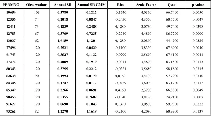
Table 1-Estimation of the annual Sharpe ratio for stocks. PERMNO identifies each stock, rho is the coefficient of the lagged variable in the autoregressive process, Qstat is the statistic for the Portmanteau test for white-noise and its respective p-value
PERMNO Observations Annual SR Annual SR GMM Rho Scale Factor Qstat p-value
Table 2 - Estimation of the annual Sharpe ratio for mutual funds. FundIdentifier identifies each fund, rho is the coefficient of the lagged variable in the autoregressive process, Qstat is the statistic for the Portmanteau test for white-noise and its respective p-value
FundIdentifier Observations Annual SR Annual SR GMM Rho Scale Factor Qstat p-value
10288 85 0,1914 0,0184 0,232 2,793 61,3 0,0167 4912 152 0,6659 0,3380 0,115 3,116 87,83 0,0000194 5029 157 0,1429 0,1490 0,0454 3,323 55,94 0,0484 5471 141 0,4669 0,1499 0,119 3,104 79,81 0,000186 5726 213 0,2944 0,0723 0,113 3,122 55,96 0,0482 5781 142 -0,0418 0,1722 0,994 1,012 1547,3 6,45E-299 5900 128 0,3773 0,1136 0,849 1,319 1457,3 7,17E-280 6131 213 0,6106 0,3362 0,305 2,602 91,96 0,00000571 6491 140 0,1813 0,0039 0,231 2,796 59,95 0,0221 6793 143 0,5048 0,6266 0,178 2,938 62,81 0,0121 6951 153 0,3881 0,2076 0,112 3,126 59,92 0,0222 7169 126 0,0265 0,0616 0,924 1,155 594,4 7,10E-100 7314 141 0,5021 0,1955 0,101 3,156 55,94 0,0484 7766 140 0,5043 0,1876 0,183 2,926 56,81 0,041 8774 213 0,1264 0,1810 0,116 3,113 97,57 0,00000103
All the funds displayed above showed presence of serial correlation. Although the
choice of the funds and stocks to be shown was random, these were drawn from the pool of
assets which showed serial correlation. This was due to the fact that the effect of serial
correlation is the main object of study of this research.
Starting with mutual funds, out of 4560, only 472 present a higher Sharpe ratio through
GMM estimation than the standard approach (about 10%). As for stocks that number goes to
1185 out of 6475 (approximately 18%). This provides some insight into how the standard
approach to estimating the Sharpe ratio may overstate the value of the ratio.
The effect of serial correlation can be seen through the scale factor. In the case of no
serial correlation (IID returns), the scaling is done by multiplying by 12, which equals 3.46 approximately. If there is positive serial correlation, the scaling factor will be lower than 3.46,
higher for negative serial correlation, as explained before. From the tables provided it can be
seen the huge impact that serial correlation can have in the aggregation process, with some of
set of results, this value ranges from a minimum of 1.58 to a maximum of 13.57, for stocks,
and 1.005 and 4.069, for mutual funds.
Additionally, by looking at the value of rho, one can get a sense of the signal of serial
correlation. If rho is positive then there is positive serial correlation, negative otherwise. Of
course, this analysis must be complemented by looking at the statistical significance of the
coefficient, together with the Partmanteu Q-statistic, to ensure that there is, in fact, serial
correlation.
In such a big sample, it is obvious not all funds and stocks would yield the presence of
serial correlation. Nonetheless, according to the Portmanteau test of white noise, 1019 mutual
funds display some presence of serial correlation in the context of the AR(1) model, which
represents around 22.35%. As for stocks, the percentage goes down to 12.28%, or 795 out of
6475. These percentages, though not huge, still represent a large part of all mutual funds and
stocks, which means that serial correlation can, in fact, impact investment decisions based on
the Sharpe ratio.
Using the values of the Sharpe ratios in Table 1 and Table 2 it can be shown that an
ordered ranking of the stocks/funds based on these values would change, depending on which
estimator of the ratio was used. The tables with this simple demonstration can be seen in the
appendix.
Discussion of the results
In line with the results obtained by Lo, it was shown that serial correlation has a
non-trivial impact when performing time-aggregation to estimate annual Sharpe ratios from monthly
data. Adding to the author’s work in terms of size of the dataset and the use of stocks instead
of the data, both in stocks and mutual funds, but also that the scaling factor to be used can vary
greatly depending on the magnitude of serial correlation.
Conclusion
The Sharpe ratio is one of the most widely used measures of risk-adjusted returns in the
financial world. A great deal of attention has been devoted to the ratio since its inception, to its
properties and how to modify it to yield better results. Several alternative measures have been
proposed. Nevertheless, it is still used as one among many indicators of performance of funds
and other assets, which says something about the usefulness of this ratio.
However, useful as it may be, it is also frequently used in a very careless manner. The
purpose of this research was to show that one needs to pay close attention to the specific
characteristics of the fund/assets’ returns, in particular, to the presence of serial correlation,
when estimating the ratio and especially when performing time-aggregation.
It was shown that indeed serial correlation plays a major role when aggregating monthly
Sharpe ratios to get an annual value by increasing or decreasing the scaling factor to be used in
such aggregation. This scaling factor can be drastically different from the standard one that is
usually used in this kind of aggregation.
Given that this ratio is, in general, used to make an ordered ranking of assets under
consideration (either to assess past performance or possible future investments) the impact of
the scaling factor is non-negligible, especially if there are many similar assets with values of
the Sharpe ratio computed by the standard approach that are close to each other. As has been
shown, such a ranking can alter significantly should one or many assets by subject to serial
correlation.
In conclusion, the Sharpe ratio is a useful measure of performance that can easily be
anyone who uses the ratio should be familiar with its assumptions and limitations. Moreover,
when performing time-aggregation of the Sharpe ratio, it is imperative to check for serial
correlation in returns, otherwise the validity of the conclusions drawn from the comparison of
ratio values might be null.
Appendix
1) Fraction of VIID due to estimation errors in 𝝁 versus 𝝈 (𝜕𝑔𝜕𝜇)0𝜎0
𝑉==>
= 1
1 +12𝑆𝑅0
(𝜕𝑔 𝜕𝜎)02𝜎9
𝑉==>
= 1 2𝑆𝑅0 1 +12𝑆𝑅0
2) Expression of the variance of Rt (q)
𝑉𝑎𝑟 𝑅' 𝑞 = 𝐶𝑜𝑣 𝑅'Kl, 𝑅'Km = 𝑞𝜎0+ 2𝜎0 (𝑞 − 𝑘)𝜌a eK*
a)* eK*
m)o eK*
3) Change in the ordering of a ranking based on the Sharpe ratio
If the estimators arrived using the standard approach and GMM were the same, the middle
columns, which contain the identifiers of the stocks and funds would be the same. However,
the ordering changes.
Ranking - Stocks
SR Standard GMM SR_GMM
1,6159 13037 93262 1,1618
1,2270 93262 13037 1,1204
0,5355 90455 12783 0,7235
0,4069 77274 90455 0,2682
0,3780 10659 12411 0,2488
0,3769 12783 80343 0,2212
0,3755 80343 77274 0,1919
0,3527 61743 10659 0,1212
0,2521 77496 61743 0,1132
0,2266 85349 91627 0,1043
0,2018 12356 12356 0,0847
0,1994 82638 85349 0,0691
0,1839 12411 77496 0,0429
0,1747 84348 82638 0,0170
0,0690 91627 84348 0,0117
Ranking Mutual Funds
Annual SR Standard GMM Annual SR GMM
0,6659 4912 6793 0,6266
0,6106 6131 4912 0,3380
0,5048 6793 6131 0,3362
0,5043 7766 6951 0,2076
0,5021 7314 7314 0,1955
0,4669 5471 7766 0,1876
0,3881 6951 8774 0,1810
0,3773 5900 5781 0,1722
0,2944 5726 5471 0,1499
0,1914 10288 5029 0,1490
0,1813 6491 5900 0,1136
0,1429 5029 5726 0,0723
0,1264 8774 7169 0,0616
0,0265 7169 10288 0,0184
References
[1] Lo, Andrew. 2002 “The statistics of Sharpe ratios” Financial Analysts Journal58(4), 36-52.
[2] Hansen, L. P. (1982). “Large sample properties of generalized method of moments estimators”. Econometrica: Journal of the Econometric Society, 1029-1054.
[3]Markowitz, H. (1952). “Portfolio selection”. The journal of finance, 7(1), 77-91.
[4] Markowitz, H. (1959). “Portfolio Selection, Efficent Diversification of Investments”. J. Wiley.
[5] Sharpe, W. F. (1963). “A simplified model for portfolio analysis”. Management science, 9(2), 277-293.
[6]Sharpe, W. F. (1964). “Capital asset prices: A theory of market equilibrium under conditions of risk”. The journal of finance, 19(3), 425-442.
[7]Sharpe, W. F. (1966). “Mutual fund performance”. The Journal of business, 39(1), 119-138. [8]Sharpe, W. F. (1994). “The Sharpe ratio”. The journal of portfolio management, 21(1), 49-58.
[9] Lintner, J. (1965). “Security prices, risk, and maximal gains from diversification”. The journal of finance, 20(4), 587-615.
[10]Lintner, J. (1965). “The valuation of risk assets and the selection of risky investments in stock portfolios and capital budgets”. The review of economics and statistics, 13-37.
[11] Treynor, J. L. (1961). “Toward a theory of market value of risky assets”. Unpublished manuscript, 6.
[12]Kothari, S. P., & Warner, J. B. (2001). “Evaluating mutual fund performance”. The Journal of Finance, 56(5), 1985-2010.
[13] Daniel, K., Grinblatt, M., Titman, S., & Wermers, R. (1997). “Measuring mutual fund performance with characteristic-based benchmarks”. The Journal of finance, 52(3), 1035-1058. [14] Smith, K. V., & Tito, D. A. (1969). “Risk-return measures of ex post portfolio performance”. Journal of Financial and Quantitative Analysis, 4(4), 449-471.
[15] Dowd, K. (1999). “A value at risk approach to risk-return analysis”. The Journal of Portfolio Management, 25(4), 60-67.
[16]Israelsen, C. (2005). “A refinement to the Sharpe ratio and information ratio”. Journal of Asset Management, 5(6), 423-427.
[17] Scholz, H. (2007). “Refinements to the Sharpe ratio: Comparing alternatives for bear markets”. Journal of Asset Management, 7(5), 347-357.
[18] Elton, E. J., Gruber, M. J., & Blake, C. R. (1996). “Survivor bias and mutual fund performance”. The Review of Financial Studies, 9(4), 1097-1120.
[19] Leland, H. E. (1999). “Beyond Mean–Variance: Performance Measurement in a
Nonsymmetrical World (corrected)”. Financial analysts journal, 55(1), 27-36.
[20]Lhabitant, F. S. (2000). “Derivatives in portfolio management: why beating the market is easy”. Derivatives Quarterly, 7(2), 39-46.
[22] Goetzmann, W., Ingersoll, J., Spiegel, M., & Welch, I. (2007). “Portfolio performance manipulation and manipulation-proof performance measures”. The Review of Financial Studies, 20(5), 1503-1546.
[23]Christie, S. (2007). Beware the Sharpe ratio.
[24]Miller, R. E., & Gehr, A. K. (1978). “Sample size bias and Sharpe's performance measure: A note”. Journal of Financial and Quantitative Analysis, 13(5), 943-946.
[25] Bao, Y., & Ullah, A. (2006). “Moments of the estimated Sharpe ratio when the observations are not IID”. Finance Research Letters, 3(1), 49-56.
[26]Fama, E. F. (1965). “The behavior of stock-market prices”. The journal of Business, 38(1), 34-105.
[27]Kacperczyk, M., & Damien, P. (2011). “Asset allocation under distribution uncertainty”. In McCombs Research Paper Series No. IROM-01-11.
[28]Boynton, W., & Chen, F. (2017). A parametric bootstrap to evaluate portfolio allocation models. Finance Research Letters.
[29]Woehrmann, P., Semmler, W., & Lettau, M. (2005). Nonparametric estimation of the time-varying Sharpe ratio in dynamic asset pricing models. Institute for Empirical Research in Economics, University of Zurich.
[30] Härdle, W., Tsybakov, A., & Yang, L. (1998). Nonparametric vector
autoregression. Journal of Statistical Planning and Inference, 68(2), 221-245.
[31]Aftab, N., Jungwirth, I., Sedliacik, T., & Virk, N. (2008). Estimating the Distribution of Sharpe Ratios. E-revir. Najdeno, 1.
[32]Andrew, W. (1999). Lo and A. Craig MacKinlay. A Non-Random Walk Down Wall Street,