Speech Features for Discriminating Stress Using
Branch and Bound Wrapper Search
Mariana Juli˜ao1, Jorge Silva1, Ana Aguiar1, Helena Moniz2,3, and Fernando Batista2,4
1
Instituto de Telecomunica¸c˜oes,
Rua Dr. Roberto Frias, s/n Porto 4200-465, Portugal. http://www.it.pt
2 INESC-ID, Lisboa, Portugal 3
FLUL/CLUL, Universidade de Lisboa, Portugal
4 ISCTE - Instituto Universit´ario de Lisboa, Portugal
[email protected],[email protected], [email protected],[email protected],fernando.batista@l2f.
inesc-id.pt
Abstract. Stress detection from speech is a less explored field than Au-tomatic Emotion Recognition and it is still not clear which features are better stress discriminants. VOCE aims at doing speech classification as stressed or not-stressed in real-time, using acoustic-prosodic features only. We therefore look for the best discriminating feature subsets from a set of 6285 features – 6125 features extracted with openSMILE toolkit and 160 Teager Energy Operator (TEO) features. We use a mutual in-formation filter and a branch and bound wrapper heuristic with an SVM classifier to perform feature selection. Since many feature sets are se-lected, we analyse them in terms of chosen features and classifier perfor-mance concerning also true positive and false positive rates. The results show that the best feature types for our application case are Audio Spec-tral, MFCC, PCM and TEO. We reached results as high as 70.36% for generalisation accuracy.
Keywords: Stress, emotion recognition, ecological data, feature sets, feature selection.
1
Introduction
The motivations for detecting stress from speech range from it being a non-intrusive way to detect stress, to ranking emergency calls [6], or improve speech recognition systems, since it is known that environmentally induced stress leads to fails on speech recognition systems [11]. Public Speaking is said to be “the most common adult phobia” [13], showing the relevance of a tool to improve public speaking. In VOCE3, we target developing such a tool, by developing algorithms to identify emotional stress from live speech. In particular, VOCE
3
corpus comes mainly from public speaking events that occur within academic context, like presentations of coursework or research seminars. The envisioned coaching application requires detecting emotional stress in live speech in near real time, to give the user timely feedback, which requires adapting the com-putational costs to the limited memory and comcom-putational resources to use. Reducing the number of features used for classification reduces the amount of data to collect, the amount of features to be extracted and the complexity of the classifier, impacting a reduction in the memory and computational resources used. Additionally, feature selection can increase the classifier’s accuracy [10]. Thus, in this paper, we focus on identifying these reduced feature sets based on their performance as stress discriminators.
The Fundamental Frequency, F0, is the most consensual feature for stress discrimination [25, 16, 7, 12], but several metrics for energy and formant changes have been proposed, often represented by Mel-Frequency Cepstral Coefficients (MFCCs) [25, 15, 6]. Frequency and amplitude perturbations – Jitter and Shim-mer –, and other measures of voice quality, like Noise to Harmonics Ratio and Subharmonics to Harmonics Ratio [22, 20] have also been used. Teager En-ergy Operator-based features have also shown to perform well in speech under stress [25, 26].
In this work, we start from the union of two feature sets: the group of fea-tures extracted using the openSMILE toolkit [19], and the group of TEO-based features, to be detailed on Sect. 3.2. We filter these feature sets with Mutual Information and then use a branch-and-bound wrapper to explore the space of possible feature sets. Finally, we analyse the best feature sets chosen on various branches for most frequently chosen feature categories.
2
Speech Corpus and Data Annotation
The VOCE corpus [2] currently consists of 38 raw recordings from voluntaries aged 19 to 49. Data is recorded in an ecological environment, concretely during academic presentations4. Speech was automatically segmented into utterances, according to a process described in [5].
Annotation into stressed or neutral classes was performed per speaker, based on the mean heart rate [4]. Utterances on the third quartile of mean heart rates for that speaker are annotated as stressed, while the remaining ones are annotated as neutral.
Using an ecologically collected corpus imposes an unavoidable trade-off be-tween the quality of the recording and the spontaneity of the speaker. Higher quality of the recording not only allows more reliable feature extraction, in gen-eral, but also impacts the performance of the segmentation algorithms we use to split the speech into sentence-like units – utterances –, and do text transcription, necessary for the extraction of TEO features. For these reasons, we chose only 21 raw recordings for this work.
4
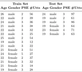
Table 1. Dataset demographic data. PSE: Public Speaking Experience, 1 - 5: 1 - little experience, 5 - large experience.
Train Set Test Set
Age Gender PSE #Utts Age Gender PSE #Utts 26 male 2 56 24 male 3 97 22 male 2 39 19 male 2 61 24 male 3 36 19 male 3 86 21 male 3 38 19 female 3 64 22 male 3 32 23 female 4 71 22 male 3 25 19 female 3 63 25 male 2 54 19 male 3 12 21 male 3 22 21 female 3 51 24 female 5 27 22 female 2 37 21 female 3 32 21 female 3 18 19 female 3 28
For these speakers, 1457 valid utterances were obtained5. The set of
utter-ances is divided into 15 speakers (507 utterutter-ances) for training and 6 speakers (442 utterances) for testing. Since the number of stressed utterances corresponds to approximately 1/4 of the total, we randomly down-sampled the train data in order to balance the two classes, which led to the mentioned 507 utterances. During feature selection, the classifier was trained on 354 utterances and tested on 153 utterances. These utterances belonged to the train set. Table 1 charac-terises the dataset concerning age, gender, public speaking experience, and the number of utterances considered6.
We performed outlier detection on each feature using the Hampel identi-fier [14] with t = 10. The outliers were then replaced by the mean value of the feature excluding outliers, and feature values were scaled to the interval [0;1].
3
Methodology
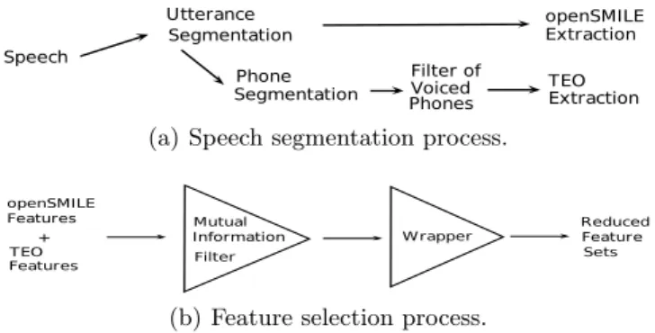
Figures 1(a) and 1(b) illustrate the workflow for speech segmentation and feature selection, respectively.
5
Remaining utterances after discarding 94 utterances with length of less than 1 second or more than 25 seconds.
6
Please note that the stated number of utterances on the train set corresponds to the one actually used after discarding a part of the neutral utterances, and not to the number of utterances in the natural set.
(a) Speech segmentation process.
(b) Feature selection process.
Fig. 1. Workflow
3.1 Acoustic-prosodic features
The set of Functional Features is “obtained by applying statistic functionals to the low-level descriptors (LLD) computed over the segment” [9, 19], and provides a total of 6125 utterance level features [19]. The LLD are “a set of 128 frame level features extracted each 10 ms from the signal” [9]. These features and their extraction processes are described in [8] and [18].
The openSMILE toolkit is capable of extracting a very wide range of acoustic-prosodic features and has been applied with success in a number of paralinguistic classification tasks [17]. It has been used in the scope of this study to extract a feature vector containing 6125 speech features, by applying segment-level statis-tics (means, moments, distances) over a set of energy, spectral and voicing related frame-level features.
3.2 Teager Energy Operator features
We extracted TEO-Based features: Normalized TEO autocorrelation envelope and Critical band based TEO autocorrelation envelope as in [25]. The literature where Normalized TEO autocorrelation envelope and Critical band based TEO autocorrelation are presented does the feature extraction for small voiced parts usually called “tokens” [25].
To work equivalently, we did a phone recognition with the delimitation of each phone [1] and used only voiced sounds.
These correspond to phones represented by the portuguese SAMPA symbols ‘i’, ‘e’, ‘E’, ‘a’, ‘6’, ‘O’, ‘o’, ‘u’, ‘@’, ‘i∼’, ‘e∼’, ‘6∼’, ‘o∼’, ‘u∼’, ‘aw’, ‘aj’, ‘6∼j∼’, ‘v’, ‘z’, ‘Z’, ‘b’, ‘d’, ‘g’, ‘m’, ‘n’, ‘J’, ‘r’, ‘R’, ‘l’, ‘L’. [23, Chap. IV.B]
These features are extracted per frame. The length of each frame is about 10ms, depending on the feature to extract. Each phone usually contains many frames and each utterance has normally many phones. Therefore, since we want to have values per utterance, we consider each feature extracted for all phones
and apply statistics to it. These statistics are: mean, standard deviation, skew-ness, kurtosis, first quartile, median, third quartile, and inter-quartile range. This process is also illustrated in Fig. 1(a). The first two columns in Table 2 summarise the feature types considered in this work7.
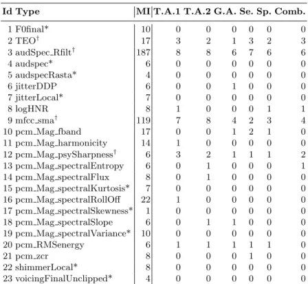
Table 2. Feature Types: Id, Name, Number of features of each type selected for MI, Number of features of each type chosen for the Best Sets: T.A.1, T.A.2, G.A., Se., Sp., and Comb. . *- Type not selected by the best sets.†- Type always selected by the best sets.
Id Type MI T.A.1 T.A.2 G.A. Se. Sp. Comb. 1 F0final* 10 0 0 0 0 0 0 2 TEO† 17 3 2 1 3 2 3 3 audSpec Rfilt† 187 8 8 6 7 6 6 4 audspec* 6 0 0 0 0 0 0 5 audspecRasta* 4 0 0 0 0 0 0 6 jitterDDP 6 0 0 1 0 0 0 7 jitterLocal* 7 0 0 0 0 0 0 8 logHNR 8 1 0 0 0 1 1 9 mfcc sma† 119 7 8 4 2 3 4 10 pcm Mag fband 17 0 0 1 2 1 0 11 pcm Mag harmonicity 14 1 0 0 0 0 0 12 pcm Mag psySharpness† 6 3 2 1 1 1 2 13 pcm Mag spectralEntropy 6 0 1 0 0 0 1 14 pcm Mag spectralFlux 8 0 1 0 0 0 0 15 pcm Mag spectralKurtosis* 7 0 0 0 0 0 0 16 pcm Mag spectralRollOff 22 1 0 0 0 0 0 17 pcm Mag spectralSkewness* 1 0 0 0 0 0 0 18 pcm Mag spectralSlope 6 0 1 1 0 0 0 19 pcm Mag spectralVariance* 10 0 0 0 0 0 0 20 pcm RMSenergy 6 1 1 1 1 1 0 21 pcm zcr 8 0 0 0 1 0 0 22 shimmerLocal* 8 0 0 0 0 0 0 23 voicingFinalUnclipped* 4 0 0 0 0 0 0
4
Searching for the Best Feature Sets
As already stated, we apply one filter to reduce the dimensionality from initially 6285 functional (OS) plus TEO features before applying the wrapper with a
7The generic designation “type” is the result of aggregating Low Level Descriptor
features with their derived functionals (e.g., quartiles, percentiles, means, maxima, minima). This procedure is, in our perspective, a way to better group and interpret the performance of the features
Support Vector Machine (SVM) classifier with radial basis function kernel and C=1008, using python library scikit-learn.
4.1 Filter: Mutual Information
There are several metrics and algorithms to compute the relevance of features on a dataset, and the choice of this metric may hugely impact the final subset of features. However, since there is a lack of a priori knowledge about filter metric adequacy to specific datasets [24], we based our choice on the work of Sun and Li et al. [21], which showed good results in terms of classification for Mutual Information (MI), a metric that measures the mutual dependence between two random variables.
Since MI is based on the probability distribution of discrete variables and our features have continuous values, we had to define a binning. We (1) defined five binning possibilities: 50, 100, 250, 500 or 1000 bins; (2) computed MI for each feature and each binarisation possibility; (3) kept features for which the MI value belonged to the higher quartile for all binarisation options. Their distribution per feature type corresponds to the third column in Table 2.
4.2 Wrapper
We designed a branch and bound wrapper to search the space of feature sets obtained from the MI filter for the combination of features that deliver the best classifier performance. This wrapper starts by searching all combinations of sets up to 10 features, keeping all that are within 1.5% accuracy of the best solution found so far. Larger feature sets are obtained by expanding the previously kept solutions with blocks of features not yet in the sets. Every time a feature subset is tested with a classification algorithm, a score is produced, which is the accu-racy, in this case. Subsets are kept and expanded if the expansion improves the previous accuracy. This search runs until the work list of feature sets with new combinations empties. This wrapper provides a better exploration of the feature set space than traditional forward and backward wrappers. Since the search space for our wrapper is much bigger than for most wrapper methods, we used parallel programming techniques to improve the throughput of the algorithm, using python’sMultiprocessing package.
5
Results and Discussion
The mutual information filter selected 487 features, distributed into types as described in the third column of Table 2. After choosing the best 280 feature sets with training accuracies below 85% from 20 processors, we looked at their distribution by feature types, which is on Fig. 2.
8
Among these 280 feature sets we looked for the ones having the best scores in each of the considered metrics9: Train Accuracy, Generalisation Accuracy, Sensitivity (Se), Specificity (Sp)10, and a Combined Metric defined as
CombinedMetric =(Se + Sp)
2 − |Sp − Se| . (1)
The need for this metric follows from the fact that it is our goal not only to have a good generalisation accuracy, but also to have high sensitivity and high specificity at the same time. This is relevant since, as we have an imbalanced test set, with much more neutral utterances than stressed utterances, it can happen that high generalisation results are due to high values of true positives, while true negatives are neglected – which is the kind of scenario we want to avoid. On Tab. 3, each line corresponds to the best feature subset for which the metric specified in the first column was found to be maximum. The two last lines correspond to baseline results, meaning the classification for the whole set of features and for the set of MI filtered features.
Columns T.A.1, T.A.2, G.A., Se., Sp., and Comb, in Table 2, correspond to the best feature sets, according to each of these metrics, as exposed in Table 3. Each of the Columns in Table 2 signs the number of features of each type (each line corresponds to a feature type).
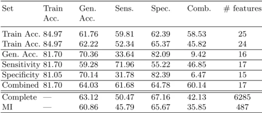
Table 3. Metrics for the Best Subsets as percentage
Set Train Acc.
Gen. Acc.
Sens. Spec. Comb. # features
Train Acc. 84.97 61.76 59.81 62.39 58.53 25 Train Acc. 84.97 62.22 52.34 65.37 45.82 24 Gen. Acc. 81.70 70.36 33.64 82.09 9.42 16 Sensitivity 81.70 59.28 71.96 55.22 46.85 17 Specificity 81.05 70.14 31.78 82.39 6.47 15 Combined 81.70 64.03 61.68 64.78 60.14 17 Complete — 63.12 50.47 67.16 42.13 6285 MI — 60.86 45.79 65.67 35.85 487
Table 3 bears the following information:
– The sets of best train accuracy do not correspond to the ones with best generalisation accuracy. Actually, these have the second worse generalisation results among these sets.
9
Generalisation Accuracy, Sensitivity and Specificity are computed on the test set.
10Being TP number of True Positives, TN number of True Negatives, FP
-number of False Positives, FN - -number of False Negatives, Sensitivity=TP+FNTP and Specificity=TN+FPTN .
– The set of best generalisation accuracy, as well as the set of best specificity, although having very good generalisation accuracies have very low sensitiv-ities. This is the kind of imbalance we want to avoid.
– The same train accuracy can have sets of very different quality. We see that for train accuracy 81.70% we have the best generalisation accuracy, the best sensitivity and the best combined metric. Looking at the other columns in the table we see that only the line for Combined Metric has acceptable results in sensitivity and specificity.
– These best reduced sets often achieve better results than both the complete set and the filtered set, having much smaller sets, which is very good for the envisioned real-time public speaking coaching application.
0 50 100 150 200 250 Vector Subsets 23 22 21 2019 18 17 16 15 14 13 12 11 109 8 7 6 5 4 3 21 Fe at ur e ty pe 0 1 2 3 4 5 6 7 # F ea tu re s
Fig. 2. Heatmap for feature type frequencies on each subset. 1 F0final 2 TEO 3 audSpec Rfilt 4 audspec 5 audspecRasta 6 jitterDDP 7 jitterLocal 8 logHNR 9 mfcc sma 10 pcm Mag fband 11 pcm Mag harmonicity 12 pcm Mag psySharpness 13 pcm Mag spectralEntropy 14 pcm Mag spectralFlux 15 pcm Mag spectralKurtosis 16 pcm Mag spectralRollOff 17 pcm Mag spectralSkewness 18 pcm Mag spectralSlope 19 pcm Mag spectralVariance 20 pcm RMSenergy 21 pcm zcr 22 shimmerLocal 23 voicingFinalUnclipped
The set of features selected by the Mutual Information filter are, grosso modo, the ones reported in the literature for other languages (e.g., [12, 26]). Those encompass pitch information, mostly final movements of pitch, audio spectral differences, voice quality features (jitter, shimmer, and harmonics-to-noise-ratio) and TEO features, the latter usually described as very robust across gender and languages. As for PCMs and MFCCs, these features are very transversal in speech processing tasks and highly informative for a wide range of tasks, not surprising, thus, for stress detection as well. The features selected by Mutual Information filter give us a more complete characterization of stress predictors. From these set the ones that are systematically chosen in the best features sets using the wrapper are mostly TEO, MFCCs and audio spectral differences. TEO and MFCCs features are also reported by [26], for English and Mandarin, as the most informative ones, even more than pitch itself.
6
Conclusions
We have used a corpus of ecologically collected speech to search for the best speech features that discriminate stress. Starting from 6125 features extracted with openSMILE toolkit and 160 Teager Energy features, we used a mutual in-formation filter to obtain a reduced subset for stress detection. Next, we searched for the best feature set using a branch and bound wrapper with SVM classifiers. Our results provide further evidence that the features resulting from the Mutual Information filtering process are robust for stress detection tasks, inde-pendently of the language, and highlight the importance of voice quality features for stress prediction, mostly high jitter and shimmer and low harmonics to noise ratio, parameters typically associated with creaky voice.
Our best result compares well with related work.
Acknowledgments. This work was supported by national funds through Funda¸c˜ao para a Ciˆencia e Tecnologia (FCT) by project VOCE (Voice Coach for Reduced Stress) PTDC/EEA-ELC/121018/2010, UID/CEC/50021/2013, and Post-doc grant SFRH/PBD/95849/2013.
References
1. Abad, A., Astudillo, R.F., Trancoso, I.: The L2F spoken web search system for mediaeval 2013. In: Proceedings of the MediaEval 2013 Multimedia Benchmark Workshop, Barcelona, Spain, October 18-19, 2013. (2013)
2. Aguiar, A., Kaiseler, M., Meinedo, H., Almeida, P., Cunha, M., Silva, J.: VOCE corpus: Ecologically collected speech annotated with physiological and psycholog-ical stress assessments. In: Chair), N.C.C., Choukri, K., Declerck, T., Loftsson, H., Maegaard, B., Mariani, J., Moreno, A., Odijk, J., Piperidis, S. (eds.) Proceed-ings of the Ninth International Conference on Language Resources and Evaluation (LREC’14). European Language Resources Association (ELRA), Reykjavik, Ice-land (May 2014)
3. Aguiar, A.C., Kaiseler, M., Meinedo, H., Abrudan, T.E., Almeida, P.R.: Speech stress assessment using physiological and psychological measures. In: Mattern, F., Santini, S., Canny, J.F., Langheinrich, M., Rekimoto, J. (eds.) UbiComp (Adjunct Publication). pp. 921–930. ACM (2013)
4. Allen, M.T., Boquet, A.J., Shelley, K.S.: Cluster analyses of cardiovascular re-sponsivity to three laboratory stressors. Psychosomatic Medicine 53(3), 272–288 (1991)
5. Batista, F., Moniz, H., Trancoso, I., Mamede, N.J.: Bilingual experiments on auto-matic recovery of capitalization and punctuation of autoauto-matic speech transcripts. IEEE Transactions on Audio, Speech, and Language Processing 20(2), 474–485 (2012)
6. Demenko, G.: Voice stress extraction. Proceedings of the Speech Prosody 2008 Conference (2008)
7. Demenko, G., Jastrzebska, M.: Analysis of voice stress in call centers conversations. Proc. of Speech Prosody, 6th International Conference, Shanghai, China (2012)
8. Eyben, F., Wllmer, M., Schuller, B.: Opensmile: the munich versatile and fast open-source audio feature extractor. In: Bimbo, A.D., Chang, S.F., Smeulders, A.W.M. (eds.) ACM Multimedia. pp. 1459–1462. ACM (2010)
9. Ferreira, J., Meinedo, H.: VOCE project stress feature survey technical report 2. Tech. rep., L2F, Inesc-ID, Lisboa, Portugal (November 2013)
10. Guyon, I., Elisseeff, A.: An introduction to variable and feature selection. Journal of Machine Learning Research 3, 1157–1182 (2003)
11. Hansen, J.H., Bou-Ghazale, S.E., Sarikaya, R., Pellom, B.: Getting started with the susas: A speech under simulated and actual stress database. Technical Report: RSPL-98-10 (1998)
12. Hansen, J.H., Patil, S.A.: Speech under stress: Analysis, modeling and recognition (2007)
13. Miller, T.C., Stone, D.N.: Public speaking apprehension (psa), motivation, and af-fect among accounting majors: A proofofconcept intervention. Issues in Accounting Education 24(3), 265–298 (2009)
14. Pearson, R.K. (ed.): Exploring Data in Engineering, the Sciences, and Medicine. Oxford University Press (2011)
15. Sarikaya, R., Gowdy, J.N.: Subband based classification of speech under stress. In: ICASSP. pp. 569–572 (1998)
16. Scherer, K.R., Grandjean, D., Johnstone, T., Klasmeyer, G., Bnziger, T.: Acoustic correlates of task load and stress. In: Hansen, J.H.L., Pellom, B.L. (eds.) INTER-SPEECH. ISCA (2002)
17. Schuller, B., Steidl, S., Batliner, A., Burkhardt, F., Devillers, L., M¨uLler, C., Narayanan, S.: Paralinguistics in speech and language-state-of-the-art and the chal-lenge. Comput. Speech Lang. 27(1), 4–39 (Jan 2013)
18. Schuller, B., Batliner, A., Seppi, D., Steidl, S., Vogt, T., Wagner, J., Devillers, L., Vidrascu, L., Amir, N., Kessous, L., Aharonson, V.: The relevance of feature type for the automatic classification of emotional user states: low level descriptors and functionals. In: INTERSPEECH. pp. 2253–2256. ISCA (2007)
19. Schuller, B., Steidl, S., Batliner, A., Nth, E., Vinciarelli, A., Burkhardt, F., van Son, R., Weninger, F., Eyben, F., Bocklet, T., Mohammadi, G., Weiss, B.: The interspeech 2012 speaker trait challenge. In: INTERSPEECH. ISCA (2012) 20. Sun, X.: A pitch determination algorithm based on subharmonic-to-harmonic ratio.
In: the 6th International Conference of Spoken Language Processing. pp. 676–679 (2000)
21. Sun, Z., Li, Z.: Data intensive parallel feature selection method study. 2014 Inter-national Joint Conference on Neural Networks (IJCNN) pp. 2256–2262 (Jul 2014) 22. Vogt, T., Andr´e, E., Wagner, J.: Automatic recognition of emotions from speech: a review of the literature and recommendations for practical realisation. In: In LNCS 4868. pp. 75–91 (2008)
23. Wells, J.: Handbook of Standards and Resources for Spoken Language Systems. Mouton de Gruyter (1997)
24. Wolpert, D.H.: The Lack of A Priori Distinctions Between Learning Algorithms. Neural Computation 8(7), 1341–1390 (Oct 1996)
25. Zhou, G., Hansen, J., Kaiser, J.: Nonlinear feature based classification of speech under stress. Speech and Audio Processing, IEEE Transactions on 9 (2001) 26. Zuo, X., Fung, P.N.: A cross gender and cross lingual study on acoustic features
for stress recognition in speech. In: Proceedings 17th International Congress of Phonetic Sciences (ICPhS XVII), Hong Kong. pp. 2336–2339 (2011)