Development of a Split Hopkinson Pressure Bar machine for high strain rate testing of bonded joints

(1)

FACULDADE DE ENGENHARIA DA UNIVERSIDADE DO PORTO

Development of a Split Hopkinson Pressure Bar

machine for high strain rate testing of bonded

joints

Alexandre José Boland

Mestrado Integrado em Engenharia Mecânica Supervisor: Prof. António Mendes Lopes Co-Supervisors: Inv. Carlos Moreira da Silva

Prof. Lucas FM da Silva

(2)

(3)

Resumo

As juntas adesivas estão a tornar-se num campo de pesquisa muito importante, pois têm muitas aplicações nas indústrias automóvel e aeroespacial, devido às suas características muito diferentes de outros processos de união. Portanto, o estudo do comportamento de juntas adesivas sob cargas de impacto é muito importante e deve ser apoiado por estudos que possam caracterizá-las corretamente.

Os membros do grupo de investigação de adesivos da FEUP, Advanced Joining Processes Unit (AJPU), estão a contribuir neste campo de pesquisa, estudando o comportamento mecânico das juntas adesivas sob diferentes tipos de solicitações, as propriedades dos adesivos e das juntas adesivas, e a influência de certos fatores, como condições ambientais, ou envelhecimento na junta adesiva. Apesar de possuir várias máquinas de teste, a FEUP precisava de um equipamento para realizar testes de impacto em alta velocidade.

Sendo assim, o principal objetivo desta dissertação é dar continuidade ao trabalho realizado por Tenreiro, que consistiu no desenvolvimento de um atuador pneumático para ser implementado numa Split Hopkinson Pressure Bar machine (SHPB). Isso inclui revisão dos desenhos mecânicos já realizados, fabricação e construção do atuador e implementação de um sistema de travagem para parar o atuador pneumático. Finalmente, é efetuado o projeto das barras que transmitirão o impacto proveniente do atuador aos provetes, tanto para o ensaio de tração como para o de compressão, bem como o projeto da estrutura de suporte da máquina.

(4)

(5)

Abstract

Adhesive joints became a very important field of research, with ample applications in the automotive and aerospace industries, due to their characteristics that are very different from other joining processes. So, studying the behavior of the adhesive joints under impact loads is very important and must be supported by studies that can correctly characterize them.

The members of the Advanced Joining Processes Unit (AJPU) at FEUP are contributing to this field of research, by studying the mechanical behavior of the adhesive joints under different types of loads, the properties of the adhesives and the adhesive joints, and the influence of certain factors, such as environmental conditions, or aging of the adhesive joint. Despite having several testing machines, the AJPU needs an apparatus to perform impact tests at high velocities.

As such, the main objective of this dissertation is to continue the work done by Tenreiro, which resumes as the design of a pneumatic actuator to be implemented in a Split Hopkinson Pressure Bar (SHPB) machine. This includes the rectification of the mechanical design, the manufacture and assembly of the pneumatic actuator, and the implementation of a braking system to stop the actuator. Finally, the design of the bars that will transmit the impact from the actuator to the specimen, for both tensile and compression tests, as well as the design of the structure to hold the machine is carried out.

(6)

(7)

Acknowledgments

Firstly, I would like to thank the Faculdade de Engenharia da Universidade do Porto for the year I spent here and for the opportunity to accomplish this dissertation, without a doubt that this made me grow up a lot in terms of knowledge and as a human being.

To all my supervisors, Prof. António Mendes Lopes, Inv. Carlos Moreira da Silva and Prof. Lucas da Silva, for all the support and data they gave me during this time.

To all AJPU’s members for the positive energy they provided, a special thanks to Dr. Eduardo Marques, Dr. Ricardo Carbas, Eng. Diogo Antunes, Eng. Paulo Nunes and Eng. António Tenreiro for their help, knowledge, and availability.

Finally, I want to thank my parents, as they are the ones who allowed me to study and supported me during this phase of my life, and also to my friends, who never left me alone during this journey.

(8)

(9)

List of Figures

Figure 2.1 - Stress distribution comparison between bonded surfaces using standard fasteners

and adhesive materials [2]. ... 3

Figure 2.2 - Block impact test apparatus [2]. ... 5

Figure 2.3 - Possible cases of impact between the hammer and the upper block [8]. ... 6

Figure 2.4 - Bertram Hopkinson experiment to measure the pressure waves [10]. ... 7

Figure 2.5 - General Kolsky compression bar apparatus [10]. ... 7

Figure 2.6 - Lagrangian diagram for SHPB compression setup [11]. ... 8

Figure 2.7 - The two most common types of loading devices of the SHPB machine [10]. ... 8

Figure 2.8 - REL's series commercialized SHPB machine [13]. ... 10

Figure 2.9 - The tensile apparatus of the SHPB machine [14]. ... 10

Figure 2.10 - Final SHPB machine, compression test setup. ... 11

Figure 3.1 – Cut view of the Pneumatic actuator assembly made on SolidWorks 2019 ... 13

Figure 3.2 - Halfway cut of the actuator's head. ... 14

Figure 3.3 - New tubular actuator's rod. ... 14

Figure 3.4 - Model of the air bushing OAV040MB [21]. ... 15

Figure 3.5 - Visualization of the rod and piston assembled on the left; on the right the assembly of the actuator's head. ... 16

Figure 3.6 - Currently pneumatic actuator developed. ... 17

Figure 3.7 - Pneumatic circuit for the actuator proposed by Tenreiro [4]. ... 18

Figure 3.8 - 3D representation of the model ACG40B-F04CG1 [27]. ... 19

Figure 3.9 - Selected valves [29], [30] [31]. ... 19

Figure 4.1 - Final model of the braking system designed on Solidworks 2019 ... 21

Figure 4.2 - Free body diagram for the dynamic study of the interaction between the actuator and the braking system. ... 22

Figure 4.3 – Matlab-Simulink model of the transmission lever. ... 23

Figure 4.4 - Stopping force along industrial shock-absorber´s stroke [32]. ... 24

Figure 4.5 - Matlab-Simulink model for node C. ... 25

Figure 4.6 - Matlab-Simulink model for node A. ... 26

Figure 4.7 - Displacement of node A obtained in the developed Matlab Simulink model. ... 27

Figure 4.8 - Velocity of node A obtained in the developed Matlab Simulink model. ... 27

Figure 4.9 - Angle produced by the transmission lever during its movement... 28

Figure 4.10 - Displacement of node C obtained in the developed Matlab Simulink model. ... 28

Figure 4.11 - Velocity of node C obtained in the developed Matlab Simulink model. ... 29

(12)

Figure 4.13 - Von Mises stress distribution obtained when a 210 kN force is applied to the

transmission lever structure, recurring SolidWorks 2019. ... 31

Figure 4.14 - Factor of safety obtained when a 210 kN force is applied to the transmission lever, recurring to SolidWorks 2019. ... 32

Figure 4.15 - Total life (cycle) obtained when a 210 kN force is applied to the transmission lever, recurring to SolidWorks 2019. ... 32

Figure 4.16 – Final model of the Skate. ... 33

Figure 4.17 - Transmission lever with the skate. ... 34

Figure 4.18 - Contact pressure obtained when a 210 k𝑁 force is applied to the Skate, recurring to SolidWorks 2019. ... 34

Figure 4.19 – Von Mises stress distribution obtained when a 210 k𝑁 force is applied to the Skate structure, recurring SolidWorks 2019. ... 35

Figure 4.20 – Factor of safety distribution obtained when a 210 k𝑁 force is applied to the Skate structure, recurring SolidWorks 2019. ... 35

Figure 4.21 - Plain bearing EGB4030-E40 specifications [33]. ... 36

Figure 4.22 - Final model of the disc springs assembly. ... 36

Figure 4.23 - Explanation of the disc spring's combinations... 37

Figure 4.24 - Various types of spring characteristics [35]. ... 37

Figure 4.25 - Single disc spring specifications [36]. ... 38

Figure 4.26 - ACE A2X6EU [32]. ... 39

Figure 4.27 - Heavy industrial shock absorber, ACE A2X6EU, specifications [32]. ... 39

Figure 4.28 - Final structure to hold the transmission lever, the skate, disc springs combination and the two shock absorbers, recurring SolidWorks 2019 ... 40

Figure 4.29 - Structures to hold the transmission lever and the disc springs with shock absorbers. ... 41

Figure 4.30 - Von Mises stress distribution obtained when a 210 k𝑁 force is applied to the central plate, recurring SolidWorks 2019. ... 42

Figure 4.31 – URES displacement distribution obtained when a 210 k𝑁 force is applied to the central plate, recurring SolidWorks 2019. ... 42

Figure 4.32 - Lateral steel plate with the groove. ... 43

Figure 4.33 - Halfway cut view of the (b) structure. ... 44

Figure 4.34 - Bearing to support the transmission lever. ... 44

Figure 4.35 - Final model of the structure that holds the transmission lever, the skate, the disc springs combination and the industrial shock absorbers. ... 45

Figure 4.36 - Final model of the Stopping car assembly. ... 47

Figure 4.37 - Actuator's rod flange. ... 47

Figure 4.38 – Stopping car position in tensile test and compression test. ... 48

Figure 4.39 - Stopping car guiding elements. ... 48

Figure 4.40 - Von Mises stress distribution obtained when a 70 k𝑁 force is applied to the stopping car, recurring SolidWorks 2019. ... 49

(13)

Figure 4.41 – Displacement distribution obtained when a 70 k𝑁 force is applied to the stopping

car, recurring SolidWorks 2019... 49

Figure 4.42 – Factor of safety distribution obtained when a 70 k𝑁 force is applied to the stopping car, recurring SolidWorks 2019. ... 50

Figure 4.43 - Stopping car linear guides... 50

Figure 4.44 - Final model of the support frame for the braking system and pneumatic actuator. ... 51

Figure 4.45 - Cross section of the 90x90H series aluminium profiles [38]... 52

Figure 4.46 - Reinforcements used on the support frame for the braking system and pneumatic actuator. ... 52

Figure 4.47 – Final braking system setup for both tensile and compression tests. ... 53

Figure 5.1 – Final model of the tensile test setup. ... 55

Figure 5.2 - Input bar and output bar for tensile tests. ... 56

Figure 5.3 - Bars support. ... 56

Figure 5.4 - Striker holder, striker tube, and loading bar assembly. ... 58

Figure 5.5 - New Split Hopkinson tensile bar design. ... 58

Figure 5.6 – Halfway cut view of the Striker holder. ... 59

Figure 5.7 – Final model of the striker tube. ... 59

Figure 5.8 – Final model of the loading bar. ... 60

Figure 5.9 - Amplified views of both ends of the loading bar... 60

Figure 5.10 - Loading bar supports. ... 61

Figure 5.11 - Final model of the Striker holder. ... 61

Figure 5.12 – Final model of the ball bearing assembly. ... 62

Figure 5.13 - Actuator's rod connector. ... 63

Figure 5.14 - Striker holder flange. ... 63

Figure 5.15 - Striker holder supports. ... 64

Figure 5.16 - Frontal view of the striker holder supports. ... 64

Figure 5.17 - Striker holder lateral support. ... 65

Figure 5.18 - Ball bearing axle for the lateral support... 66

Figure 5.19 - Striker holder vertical support. ... 66

Figure 5.20 - Cross section of the 45x45H series aluminium profiles. ... 67

Figure 5.21 - Block that holds both ball bearings... 67

Figure 5.22 - Final model of the compression test setup. ... 68

Figure 5.23 - Input bar and output bar for compression tests. ... 69

Figure 5.24 - Striker holder and striker bar assembly. ... 70

Figure 5.25 - Final model of the striker holder... 70

Figure 5.26 – Actuator’s rod connector. ... 71

(14)

Figure 5.28 - Final model of the momentum trap... 72 Figure 5.29 - Frontal view of the momentum trap without the brass pin. ... 72 Figure 5.30 – Final model of the support frame for tensile and compression setup. ... 73 Figure 5.31 - Cross section of the aluminium profiles that compose the support frame for tensile and compression setup. ... 74 Figure 5.32 - Stopper used to give alignment to the tensile and compression setup. ... 74 Figure 5.33 - Final model of the tensile and compression setup. ... 75

(15)

List of Tables

Table 2.1 - Mechanical properties and respective impact tests used [3]. ... 4

Table 2.2 - Impact test classification according to impact testing velocity [3]. ... 5

Table 3.1 - OAV040MB air bushing specifications [21]. ... 15

Table 3.2 – “O”-rings specifications [23]. ... 15

Table 3.3 - Rod seal specifications [24]. ... 16

Table 3.4 - Fasteners used to assemble the pneumatic actuator. ... 16

Table 3.5 - Pressurized gas reservoir characteristics [26]. ... 18

Table 3.6 - Air filter and regulator specifications [27] , [28] . ... 19

Table 3.7 - SMC VP742K-5YOD1-04 Valve specifications [29]. ... 20

Table 3.8 - SMC EAQ5000-F06-L valve specifications [30]. ... 20

Table 3.9 - SMC XTO-674-04E valve specifications [31]. ... 20

Table 4.1 - Parameters values inserted in the developed Matlab Simulink model, considering a maximum actuator velocity of 30 m/s. ... 26

Table 4.2 - Fasteners used to assemble the transmission lever. ... 33

Table 4.3 - Fasteners used to connect all parts and assemble the skate to the transmission lever. ... 36

Table 4.4 - Plain bearing specifications, PCM 606560 M [37]. ... 45

Table 4.5 - Fasteners used to assemble the structure. ... 46

Table 4.6 - Fasteners used to assemble the stopping car. ... 51

Table 4.7 - Fasteners used to assemble the support frame. ... 53

Table 5.1 - AISI 4140 steel chemical composition. ... 57

Table 5.2 - Physical properties of AISI 4140 steel. ... 57

Table 5.3 - Ball bearing 628-2Z specifications [40]. ... 62

Table 5.4 - Ball bearing 6205-2Z specifications ... 65

Table 5.5 - Fasteners used to assemble the Tensile setup. ... 68

Table 5.6 - Fasteners used to assemble the Compression setup. ... 73

(16)

(17)

Acronyms

SHPB Split Hopkinson Pressure Bar AJPU Advanced Joining Processes Unit

TAST Thick Adherent Shear Test

DCB Double Cantilever Beam test

ATDCB Asymmetric Tapered Double-Cantilever Beam

SENB Single-Edge Notched Beam test

CT Compact Tension test

(18)

(19)

1. Introduction

1.1. Context and Motivation

The utilization of adhesive bonding has become very important in the last century, even though this method was already known in ancient times. An adhesive is an organic or inorganic substance capable of bonding two dissimilar surfaces, creating a strong mechanical connection [1].

Adhesive joints are now generally adopted in several industries, such as automotive, aerospace, electronics, and naval, where lightweight structures are needed because of the different properties adhesives have, when compared to other types of joining processes, as welding, riveting, or screwing [2]. Adhesives have the ability to join dissimilar materials, such as composites, that cannot be joined efficiently using other conventional methods.

Since this is a relatively new field and many products that use these bonds are required to perform under sustained impact loads, it is of great importance to understand the behavior of adhesives joints under high strain rate loads. This is not straightforward, as the mechanical behavior of the adhesive structures vary significantly with the strain rate. The mechanical behavior of the joint materials can only be fully characterized as a function of the strain rate [3].

To contribute to this new field of research, the Advanced Joining Processes Unit (AJPU) at FEUP, needs the adequate equipment to correctly characterize adhesives under specific impact loads, thus, a high impact test machine is needed.

1.2. Objectives

The dissertation focus is to continue the work done by Tenreiro [4], in a previous master dissertation, into further developing a high impact test machine: a Split Hopkinson Pressure Bar machine (SHPB).

The work done by Tenreiro [4] addressed the design of a pneumatic actuator, capable of reaching high velocities, of the order of 30 m/s.

In addition to this specification, the machine should also have a variety of subsystems that help in the execution of the machine’s action. So, it is required to manufacture the pneumatic actuator, design and build a braking system to stop the pneumatic actuator, develop a structure that holds the machine, and design the assembly of the bars that will transmit the impact from the actuator to the specimen, for both tensile and compression tests.

(20)

1.3. Methodology

Initially, an evaluation of the drawings of the pneumatic actuator was made. For that purpose, the master dissertation of Tenreiro [4] was analyzed and the requirements to start the project were identified.

Although the design of the pneumatic actuator was already done, some drawings still needed adjustments for their manufacture. So, the first task was to finish all the actuator’s mechanical drawings and order the materials for their fabrication. All the pneumatic components to build the pneumatic actuator were also ordered.

After that starting stage, the design of a braking system was needed to stop the actuator, and after that, the design of the bar’s assembly that transmit the impact to the specimen for tensile and compression tests.

Lastly, the design of the support frame that holds the machine was developed.

1.4. Dissertation Outline

This dissertation is organized into six chapters, each one covering a different topic that is considered relevant to better understand the work done.

A brief introduction to the project is presented in this first chapter.

The second chapter addresses the literature review about adhesives, impact tests for adhesive joints, and commercial SHPB machines.

The third chapter describes the development of the pneumatic actuator, which includes the final design and its assembly, as well as the acquisition of the pneumatic components.

In chapter four, it is described the development and design of the braking system to stop the pneumatic actuator, as well as the support frame for both.

Chapter five describes the design of the bars that transmit the impact from the actuator to the specimen, for both tensile and compression tests, as well as the support frame.

Finally, in chapter six, this dissertation will be concluded and some proposals for future works on AJPU’s SHPB machine are presented.

(21)

2. Literature Review

In this chapter, a literature review on adhesives, different types of impact tests on adhesive joints, and commercial SHPB machines are presented.

2.1. Adhesives

Adhesives are capable of creating a strong mechanical connection between two bodies with different surface characteristics, known as substrates. There are many advantages in favour of adhesive bonding when compared to other structural joining methods, such as riveting, welding, or fastening. They allow a very smooth stress distribution along the bonded area, enabling higher fatigue resistance, since there are no concentration zones of stress caused by the holes in the surface of the substrates, as it happens with rivets or screws, Figure 2.1. Bonded structures also offer the ability of flexible joint design and they contribute to weight reduction, since dissimilar materials, such as composites, can be effectively joined [2, 5].

Figure 2.1 - Stress distribution comparison between bonded surfaces using standard fasteners and adhesive materials [2].

There are some disadvantages as well, such as low stability in humidity or extreme temperatures conditions. Moreover, adhesives require surface preparation, long curing times, and have a low resistance to perpendicular forces [2].

Although all these disadvantages were enumerated, the use of adhesives is increasing in many industries, such as aerospace, automotive, naval, and electronics [6]. Many industries manufacture components that are expected to sustain and perform adequately under impact loads. Therefore, studying the behavior of adhesive joints under high strain rate loads is important to understand and optimize the adhesives.

(22)

2.1.1. High strain rate testing

Studying the mechanical behavior of adhesives under high strain rates varies significantly. Therefore, to fully characterize the behavior of the adhesive joints as a function of the strain rate to understand the mechanical behavior of the joint under the impact load is needed [3].

Most adhesives are known for being strain rate dependent, which is caused by the inherent viscoelastic behavior of the polymeric structures, which causes the mechanical behavior to be highly sensitive to the loading rate.

Many experiments were made in previous years, by several authors, concluding that the mechanical properties of adhesives change at higher strain rates. Different tests, like tension tests, ARCAN tests, tension-torsion and tensile-compression tests on SHPB machines, showed a tendency of adhesives to change from ductile to brittle behavior as the strain rate increases. In terms of the fracture toughness, it tends to reduce as the strain rate increases [3]. All tests confirmed that the strain rate has a very significant effect on the mechanical properties of the adhesives.

2.2. Impact test for adhesive joints

Studying the behavior of adhesives under high impact loads is very complex, as it is very difficult to replicate high strain rate conditions experimentally, therefore bringing high costs to the testing, where it is required many sensors and data acquisition systems.

It is often needed to know how the adhesives will perform under different high strain rate loads and impact tests performed on bulk adhesives, to check the properties of an adhesive [2]. These types of tests are capable of determining the type of failure obtained in the joint, validate the effectiveness of the surface treatment and the energy absorption, as well as many other aspects. Therefore, many different testing devices have been developed and they can be divided into two different groups: impact tests, to determinate the properties of the adhesive; and impact tests, that can test the behavior of a complete adhesive joint [3].

As mentioned before, knowing the mechanical properties of adhesives is fundamental to design an adhesive joint under high impact loads. The most important properties, and the main tests that allow the determination of these properties, are presented in Table 2.1.

Table 2.1 - Mechanical properties and respective impact tests used [3].

Measured properties Tests

Tensile stiffness and strength Tensile test

Shear stiffness and strength TAST, Torsion, ARCAN

Fracture toughness (Mode I) DCB, ATDCB, SENB, CT

Fracture toughness (Mode II) ENF

(23)

Using these types of tests that are capable to study the properties of adhesives, isolated from other factors, are important, but assessingthe impact behavior on the adhesive joint is also extremely important. This is particularly true, when surface preparation, joint geometry, and adherent properties are considered. Therefore, the tests that are used to determine the adhesive joint behavior under high impact loads can be categorized in terms of impact velocity as it is shown in Table 2.2 [3].

Table 2.2 - Impact test classification according to impact testing velocity [3].

Test classification Testing speed Suitable test equipment

Low velocity Up to 5 m/s Pendulum impact machine

Medium Velocity Between 5 and 10 m/s Drop weight machine

High velocity Between 10 and 100 m/s SHPB machine

2.2.1. Pendulum impact test

The block impact test consists of an upper block that is bonded with an adhesive with a larger block, which is attached to a base, then the pendulum will strike the upper block in a parallel direction to the bonded surface. The energy lost by the hammer allows obtaining the energy required to fracture the specimen. This type of test is shown in Figure 2.1, and has the same principle as other impact tests, like the Charpy Impact test and the Izod impact test [2].

Figure 2.2 - Block impact test apparatus [2].

There are three different possible cases of contact between the hammer and the specimen, found by Adams and Harris [7], which can be seen in Figure 2.3. In cases, II and III where the hammer and the upper block aren’t completely aligned, peeling occurs, which means that the results obtained don’t correspond with a pure shear loading. In case I, when the hammer hits perfectly the upper block, the stress along the bond is still not constant. From that, Adams and Harris [7] concluded that, even though this type of testing is still very useful to compare the behavior of different types of adhesives, the results shouldn’t be interpreted as absolute information about the energy absorption of the bond [2].

(24)

Figure 2.3 - Possible cases of impact between the hammer and the upper block [8].

2.2.2. Drop weight test

Drop weight tests are another example of an impact test, which consists of the release of a drop mass, from a previously defined height to the adhesive joint, and depending on how it is fixed in the structure, the specimens can be tested with tensile or compression loads. The kinetic energy from the impactor, that will hit the specimen, is the same as the potential energy before the impactor is released. If the drop weight machine has an acceleration unit sub-system, it will increase the impact of energy, because of the elastic mechanism. To prevent posterior impacts from the impactor, an anti-rebound system is implemented in the drop weight machines [9].

The use of piezoelectric sensors is required to measure the impact loads on these tests. Usually, a load cell or an accelerometer creates an electric charge that is directly proportional to the mechanical load applied to a piezoelectric material. Normally they are made of ceramic or crystal quartz [9].

2.2.3. SHPB test

Another type of impact test and the most important one for this dissertation is the Split Hopkinson Pressure Bar machine, which is a test machine dedicated to study the dynamic behavior of materials under medium and high strain rates (0,5 – 5 x 103 s-1). The original concept developed by B. Hopkinson, shown in Figure 2.4, consisted of striking one of the ends of a long and thin bar, placed horizontally, with a projectile. This would generate a pressure pulse that would propagate to the other end of the bar, which would be attached to a cylinder that would later be projected against a ballistic pendulum capable of measuring the contained momentum [2].

(25)

Figure 2.4 - Bertram Hopkinson experiment to measure the pressure waves [10].

Later, Kolsky (1949) developed a new variant of the technique used by Hopkinson, which is the most common nowadays. Kolsky added a second bar to the Hopkinson pressure bar apparatus, placing the specimen between the two bars. This new mechanism consists of three major components, represented in Figure 2.5, which are the loading device, the bar components, composed of the incident bar, the transmission bar, and the momentum trap, and the data acquisition and recording system [10].

Figure 2.5 - General Kolsky compression bar apparatus [10].

The striker is fired from the gas gun and will hit the incident bar, also called the input bar, generating a pressure pulse that is transmitted to the specimen, where some energy originated by the impact will be reflected. The energy that is propagated to the specimen will then be transmitted to the transmission bar, also known as the output bar. Figure 2.6 shows the basic setup of a SHPB for the compression test and it is possible to visualize the propagation of the pulses through time [11].

(26)

Figure 2.6 - Lagrangian diagram for SHPB compression setup [11].

The loading device should be stable, controllable, and repeatable. Two different methods are commonly used, the static loading and dynamic loading, both represented in Figure 2.7. In the static loading method, the incident bar is statically loaded in pre-compression, and the energy stored is released into the incident bar. Therefore, the compression wave propagates towards the specimen. The dynamic loading method, which is the most common method, is to launch a striker that will impact the incident bar, generating the same compression wave towards the specimen. Gas guns and pneumatic actuation systems are mostly used because of their efficiency, they are safe and controllable, but other systems are used, such as electromechanical linear actuators and hydraulic systems [10].

Figure 2.7 - The two most common types of loading devices of the SHPB machine [10].

The bar components are all typical fabricated in the same material and have the same diameter, to ensure one-dimensional wave propagation. The bars must be perfectly aligned and free to move on their supports, with minimized friction. The incident bar should be, at least, twice as long as the striker bar, to avoid overlapping incident and reflected pulses [10].

In terms of data acquisition and recording system, the standard solution found is the use of strain gages to measure the strain in the bars, where two strain gauges are attached symmetrically on the surface of the bars close to where the specimen is being held. With the use of a Wheatstone bridge, the signals are conditioned. Since the voltage from the Wheatstone bridge has low amplitude, there is the need to use an amplifier. Later, the amplified signals are recorded with an oscilloscope or a high-speed data acquisition system. Digital Image Correlation (DIC) has recently been implemented in experimental SHPB setups, which is a non-contact measurement method that allows measuring the specimen’s deformations. In this

(27)

method, a pattern with high contrast is applied and with a high speed camera, it is possible to obtain images of the changes in the deformation of the specimen [10].

2.3. Commercial SHPB machines

There’re many models of SHPB machines available in the market. Even if they are not designed to test adhesive joints, they can still be used for that purpose. The main differences between the machines are their specifications, like the maximum impact velocity obtained with a gas gun, the dimension of the bars, and different equipment for the data acquisition system. Most of the companies sell this type of machine as a complete package with different speed ranges to satisfy the needs of various customers. In this section, some commercial SHPB machines are presented around the same impact speed, of 30 m/s, which is required for the development of this machine’s dissertation, as well as the solution developed in this dissertation.

2.3.1. THIOT Ingenierie - Split Hopkinson

The SHPB machines developed by THIOT Ingenierie [12], have a great variety of different testing conditions for the materials to be tested.

Their testing machines are specially designed for characterizing the dynamic behavior of materials subjected to high strain rates, using either tensile or compression testing, and are equipped with sophisticated measurement systems for high quality signal acquisition. In compression testing, they can reach strain rates from 500 to 10000 s-1_{, and in tensile testing, up}

to 3000 s-1 in less than 25 μs.

As mentioned before, the specifications of the SHPB machine are determined by the customer’s need. The model manufactured by THIOT, which corresponded to AJPU’s requirements to test adhesive joints at 30 m/s, was a turnkey gas launcher with 26 mm of diameter capable to operate up to 30 m/s and project a striker bar of 20 mm diameter. the estimated cost is of 37000 €. The gas launcher was fully-automated with a control panel, which allowed to adjust all the settings in just a few minutes and is capable of working for tensile tests and compression tests. There was as well as a velocity measurement system with optical barriers and mechanical supports for 17000€.

2.3.2. REL – Split Hopkinson

REL [13], is another company that also sells equipment for impact testing at high strain rates, from 100 to 10000 s-1_{at compression tests. Figure 2.8, shows the REL’s series SHPB}

machine for compression testing.

When asked for a gas gun capable of testing specimens with impact velocities of 30 m/s the solution given had a price tag of 27000 € and consisted of a bar accelerator automation package, two bar accelerator adapters, each one for compression and tensile testing, and a barrel.

(28)

Figure 2.8 - REL's series commercialized SHPB machine [13].

2.3.3. Natural Impacts Ltd – Split Hopkinson

Natural Impacts had an SHPB apparatus that wanted to sell, presented in Figure 2.9. The price of the apparatus for tensile and compression testing was of 55200 €. The compression apparatus consisted of input and output bars of 16 mm diameter by 1200 mm long, with a 500 mm long striker bar, all made of silver steel. The launcher is powered by compressed air capable to reach 30 m/s and a velocity meter. The data acquisition system with amplifiers and the control system was fired from a remote control panel, which would fill and maintain the required pressure. The tensile apparatus had an input and output bar with 16 mm of diameter made of titanium 64, where the input bar is 3000 mm long, and the output bar 1200 mm long. The striker, made of titanium 64 as well, has a length of 700 mm. The launcher was a twin-cylinder launcher, powered by compressed air capable of only 20 m/s. The data acquisition was the same as the one used for tensile testing.

(29)

2.3.4. AJPU’s SHPB machine

The development of the SHPB machine was firstly initiated by Tenreiro [4], with the development of a pneumatic actuator to be the loading device of the machine. This one is capable to operate at up to 30 m/s, for both tensile and compression tests. The need to design a SHPB machine grew, not only for the necessity of means to experiment with adhesive joints but also for enabling students to consolidate the gathered knowledge during their master’s degree.

The initial point was to validate and correct the mechanical drawings to manufacture the pneumatic actuator. After this verification process, it was required to develop a braking system to stop the actuator’s rod movement under 300 mm of available length and work as well for tensile and compression tests. Finally, to build a support frame to hold the pneumatic actuator and his braking system.

The bar components for compression and tensile tests had to be designed and a second support frame, to hold the bar components, had to be developed, to avoid transmission of vibrations from the actuator to the bar’s testbed.

All the developments on the SHPB machine are fully described in the next chapters, and the final product is presented in Figure 2.10, which shows the compression test setup with the tensile bar’s setup on the side, fixed to the support frame.

(30)

(31)

3. Pneumatic actuator

This chapter describes the design and the validation process for the building of the pneumatic actuator as well as the selection and acquisition of the pneumatic components for its construction.

3.1. Pneumatic Actuator construction

As it was previously said, Tenreiro [4] made the initial design of a pneumatic actuator that would be used on a SHPB machine. However, that design had some flaws that needed to be corrected. As such, the initial tasks for this dissertation were to carefully analyze his work, to correct the mechanical drawings previously made, that can be seen in Appendix B, and finally to choose materials for their fabrication. All these initial tasks were done with the help of

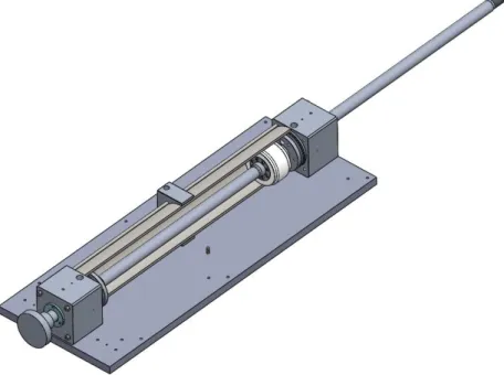
SolidWorks 2019 and the final design of the pneumatic actuator can be seen in Figure 3.1.

Figure 3.1 – Cut view of the Pneumatic actuator assembly made on SolidWorks 2019

This actuator consists of a rod that is supported by air bushings to prevent any physical contact between components. The cylinder wall should also have no contact as well with the piston. In both stroke ends, there is a sealed damping chamber that allows the start of the rod´s motion without air flowing out of the chamber.

The major changes done were to correct the mechanical drawings of the actuator’s head, namely the inner diameters where the air bushings would be inserted and the channels for outflow and inflow for the air bushings, as they can be seen in Figure 3.2.

(32)

Figure 3.2 - Halfway cut of the actuator's head.

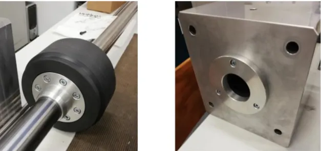
Previously the rod’s actuator was defined to be built in aluminium Alloy 6063-T6 to maintain rigidity and minimize the weight, but the problem was that it wasn’t possible to guarantee these characteristics and respect the tolerances along the full length of the rod. The solution found was to change the 40 mm diameter aluminium shaft to a heat-treated H6 tubular shaft steel from Bosch Rexroth [15] with an inside diameter of 26.5 mm while maintaining the 40 mm of outside diameter to continue to be compatible with the air bushings previously chosen, Figure 3.3. The rod has also threaded ends to allow the connection with the assembly that will launch the striker bar and in the other end where it will provide the contact with the braking system. The rod’s weight is around 14 kg.

Figure 3.3 - New tubular actuator's rod.

To build the pneumatic actuator, after all of the mechanical drawings were reviewed, the order of all the materials was needed. So, all the Aluminium components and the Nylatron GSM for the piston were bought from Polylanema [16], and the steel components from Ramada Aços [17]. The cylinder wall was bought from Teclena [18], and the actuator’s rod was bought from Equinotec [19]. Some parts were able to be manufactured by FEUP mechanical

(33)

engineering department workshop and the rest was sent to Tecnogial [20], like the cylinder wall and the two actuator’s heads. The air bushings were bought from OAV bearings [21]. This bearing has a core made of graphite, where a rod passes through it, Figure 3.4, and their specifications are shown in Table 3.1.

Figure 3.4 - Model of the air bushing OAV040MB [21].

Table 3.1 - OAV040MB air bushing specifications [21].

The static “O”-rings used in each actuator’s head to remove the possibility of air leaking through gaps between the cylinder wall and the head have their specifications shown in Table 3.2. From the rod, seal specifications can be consulted as well. All these components were bought from Rovandi [22]. A 72 Shore A material hardness was enough, as the pressure is quite low and the gaps between the cylinder body and heads are small.

Table 3.2 – “O”-rings specifications [23].

Reference 445 642 14 452 149

d1 [mm] 40 136

d2 [mm] 1.50 3

Material 72 NBR 872 72 NB 72 NBR 872 72 NB

The rod seal was selected to prevent the leakage from the pneumatic damping chamber during the star of the piston’s motion and its specifications can be consulted in Table 3.3.

(34)

Table 3.3 - Rod seal specifications [24].

All the fasteners used to connect the parts were bought from Fabory [25], and the list is represented by Table 3.4

Table 3.4 - Fasteners used to assemble the pneumatic actuator.

Element Norm Qt. Screws ISO 4762 M4x10 - 8.8 6 ISO 4762 M6x20 - 8.8 16 ISO 4762 M10x60 - 8.8 2 Nuts ISO 4032 - M10-8 8 Washer W10 NF 25-515 8

After the parts were manufactured it was possible to mount the pneumatic actuator. The following Figure 3.5 shows the actuator’s rod mounted with the piston as well as the actuator’s head.

Figure 3.5 - Visualization of the rod and piston assembled on the left; on the right the assembly of the actuator's head.

However, it is only possible to visualize the pneumatic actuator without its sitting table because at the time of writing that table was still being designed to complement the rest of the assembly of the SHPB machine. The pneumatic actuator can be seen in Figure 3.6

(35)

Figure 3.6 - Currently pneumatic actuator developed.

3.2. Pneumatic components

At the same time that the actuator was being built, the pneumatic components had to be ordered. Most of the components were already selected by Tenreiro [4] but some changes had to be made to fit properly with the construction of the actuator itself.

The pneumatic circuit proposed by Tenreiro [4], is presented in Figure 3.7, and the cost of acquisition of all the pneumatic components was around 800 €.

(36)

Figure 3.7 - Pneumatic circuit for the actuator proposed by Tenreiro [4].

The actuator had to have a stable supply of air without pressure variations. Therefore, the supply line was unable to deliver a flow of air steady enough for all the actuator travel. A dedicated reservoir was selected with a computed capacity of 60 liters, component 1.1 from the pneumatic circuit. It was chosen a gas reservoir from Amtrol-Alfa [26], its characteristics are summarized in Table 3.5.

Table 3.5 - Pressurized gas reservoir characteristics [26].

Air filter and pressure regulator were needed to regulate and maintain a clean air mass flow to work in normal conditions and to ensure stable functioning conditions. Therefore, an air filter pressure regulator is selected for the main pneumatic circuit and another air supply unit to regulate the airflow for the air bushings, that operate at a different pressure.

(37)

The air filter and regulator combination, 1.3 and 2.1 from the pneumatic circuit, to be implemented in the main pneumatic circuit is the model ACG40B-F04CG1 manufactured by SMC. Figure 3.8 shows a 3D representation of this unit.

Figure 3.8 - 3D representation of the model ACG40B-F04CG1 [27].

For the air bushing pneumatic supply, the selected model is ACG20B-F02CG1 manufactured by SMC as well [28]. The Table 3.6 presents the most important specifications of these two units.

Table 3.6 - Air filter and regulator specifications [27] , [28] .

To command the actuator, it was required two directional valves, represented as 1.4 and 1.5 from the pneumatic circuit, and two quick exhaust valves, 1.6 and 1.7, where each one controls the mass flow that enters the chamber to which they will be connected. The quick exhaust valves will allow the air to flow from the chamber to the atmosphere as quickly as possible giving the actuator’s rod the ability to reach high accelerations. The selected valves are shown in Figure 3.9, and all their specifications can be consulted in Table 3.7, Table 3.8, and Table 3.9.

(38)

Table 3.7 - SMC VP742K-5YOD1-04 Valve specifications [29].

Table 3.8 - SMC EAQ5000-F06-L valve specifications [30].

(39)

4. Braking system

As the name suggests, the braking system is needed to stop the pneumatic actuator. The pneumatic actuator can operate at 30 m/s, so there must be some kind of a braking system to stop it and to decrease 30 m/s to a maximum of 5 m/s, which is the maximum velocity that an industrial shock absorber can support. This braking system also has to be able to stop the actuator movement within 300 mm of travel, because it was the length available to drive the actuator to stop. The idea was to build a lever system, which is one of the six simple machines identified by Renaissance scientists, that could reduce the velocity.

In this case, a ratio of 1:6 would reduce the velocity from those 30 m/s to 5 m/s, but the forces on the shock absorber were very high since they would be 6 times higher, so the ratio had to decrease. By doing that the velocity on the contact point with the shock absorber would increase, so to help the stoppage and still reaching the 5 m/s, the use of a spring connected to the shock absorber is also needed.

To know the length of the transmission lever, the spring stiffness, and the shock absorber force, a dynamic study of the interaction between the actuator and the braking system was needed. This study leads to a 4th_{order differential equation system, so it is impossible to}

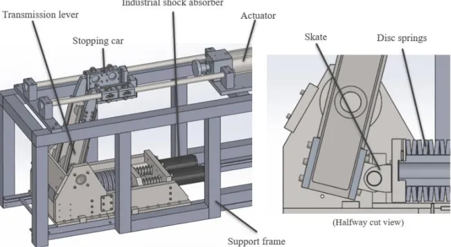
evaluate without a simulation, that is why this system was simulated in Matlab Simulink. This chapter describes the design of the braking system and all the tasks were done with the help of Matlab Simulink and SolidWorks 2019. The final design of the braking system can be seen in Figure 4.1 and all the mechanical drawings can be consulted in Appendix C, D, and E.

(40)

4.1. System equations

To initiate the dynamic study, a free body diagram, Figure 4.2, was defined to identify all the interacting forces.

Figure 4.2 - Free body diagram for the dynamic study of the interaction between the actuator and the braking system.

4.1.1. Transmission lever

In one end of the transmission lever would be the contact point with the actuator, node A, on the other end would be the point of contact with the spring, node B. Node C represents the contact point between the spring and the shock absorber. The distance from the center of rotation of the transmission bar to the contact with the actuator is represented by l1, the distance

to the contact point with the spring represented by l2, and d, represents the distance from the

center of the mass of the transmission lever to the center of rotation. The length of the transmission lever is represented by lb, and can be defined as:

lb = l1 + l2 (4.1)

The transmission ratio is represented by i, and can be defined as: i = l1

l2 (4.2)

Where l1 and l2 can be defined by:

l2 = l𝑏

i+1 ; l1 = l𝑏− l𝑏

(41)

The distance from the center of the mass of the transmission lever to the center of rotation can be determined by the combination of previous equations:

d = l𝑏

2 − l1

i (4.4)

The momentum of inertia of the transmission lever was approximated to a moment of inertia from a circular bar, where mb represents the mass of the bar. Combined with the Steiner

theorem, the following expression is defined by: I = mb (

l2 12+ 𝑑

2₎ _(4.5)

The actuator was designed to be stopped under 300 mm, so the node A can only travel at maximum, 300 mm. θ represents the angle produced by the transmission lever during its movement. Knowing this, it can be achieved by the following expression:

θ = sin−1₍𝑥𝐴

l1) (4.6)

To represent the acceleration force of inertia produced from the transmission lever, it can be defined by:

Faciner= cos θ ∗ I α

l1 (4.7)

Where α stands for the angular acceleration of the transmission lever:

α =

𝑥̈A

l1 (4.8)

All previous expressions were introduced into the Matlab Simulink software as it can be seen in Figure 4.3. In Appendix A is depicted the implemented dynamic model, in Matlab

Simulink, to its full extent, as well as the results.

(42)

4.1.2. Shock absorber

Since all the parameters of the transmission lever were defined, it was time to define the parameters from the shock absorber and the spring.

In the case of the shock absorber, the industrial shock absorbers from ACE manufacturer show that the force of this component is constant along the whole stroke, as it can be seen in Figure 4.4. This is just a generical graph from ACE manufacturer to illustrate the behavior of their industrial shock absorbers [32].

Figure 4.4 - Stopping force along industrial shock-absorber´s stroke [32].

Where Umáx, is the dissipated energy by the absorbers per cycle, s is the

shock-absorbers stroke, 𝑥_𝑠𝑎 the maximum speed that the shock absorber operates at, and 𝑥_𝐶̇ the velocity of the point of contact between the springs and the shock absorber. All these characteristics can be correlated, and the force of the shock absorber can be defined as:

Fsa =

𝑈𝑚á𝑥

𝑠∗ 𝑥𝑠𝑎

𝑥̇

𝑐 (4.9)

In the Matlab-Simulink was introduced a small detail, where the Fsa would be calculated

if the displacement of the node C, xC was positive or null. If the displacement was negative, the

value of the Fsa would be 0.

4.1.3. Spring

The calculation of the force of the spring, Fm, needed the rigidity of the spring, km, the

displacement of the node B, the contact point between the transmission lever and the spring, and the displacement of node C:

Fm = km (xb-xc) (4.10)

Where xb:

xB = 𝑥𝐴

(43)

4.1.4. Differential equations of node C and A

To determinate the acceleration of node C, an equilibrium of forces had to be made and the following equation was defined:

a

C =

𝐹_𝑚− 𝐹_𝑠𝑎

𝑚𝑠𝑝𝑟𝑖𝑛𝑔

(4.12)

All previous expressions were introduced into the Matlab Simulink software and can be seen in Figure 4.5.

Figure 4.5 - Matlab-Simulink model for node C.

The force of the shock absorber, the force of spring, and the acceleration force of inertia produced from the transmission lever were correlated with an equilibrium of forces as well, where m1 and m2 represent the masses of the actuator rod and the stopping car used to make the

contact between the actuator and the transmission lever: (m1+m2) aA + FmA + Faciner = 0

aA

=

−𝐹𝑚𝐴 − 𝐹𝑎𝑐 𝑖𝑛𝑒𝑟

m1+m2

(4.13)

Where FmA is the force of spring, Fm divided by i. From this previous equation, the value

of aA could be determined, and aA and aC were defined, just by using a second-order integrator.

This integrator is limited in velocity and position to eliminate numerical problems during the stoppage of the system. Those accelerations obtained could give the values for the velocities and displacements for nodes A, B, and C. That correlation is represented in Figure 4.6.

(44)

Figure 4.6 - Matlab-Simulink model for node A.

4.1.5. Simulation results

Since all the system equations were defined, the parametrization of the system must be accomplished, followed by experimenting with different spring rigidities, different shock absorber forces, and different lengths for the transmission lever. All this process was iterative and, in the end, to have a proper correlation from parts dimensioning and simulation values, a search of specific springs characteristics and shock absorber had to be made. This meant to introduce values from catalogs found during this search for the spring and shock absorber. To better characterize the transmission lever on the Matlab Simulink software, it was used

Solidworks to design the transmission lever. With this, the value of the momentum of inertia

and mass of the bar were manually introduced in the Matlab Simulink software.

All the values for all parameters were inserted in the Matlab Simulink model to be able to define the system and find a solution for the dimensioning of the shock absorber, the spring, and transmission lever, as shown in Table 4.1.

Table 4.1 - Parameters values inserted in the developed Matlab Simulink model, considering a maximum actuator velocity of 30 m/s.

Parameters Values

m1 (actuator rod mass) [kg] 14

m1 (stopping car mass) [kg] 4

lb (length of transmission lever) [m] 0.8

i (transmission ratio) [-] 3:1

mb (transmission lever mass) [kg] 46.1 I (momentum of inertia of the transmission lever) [kg*m2_] _3.043 d1 (distance from the center of the mass of the transmission bar

to the center of rotation) [m] 0.12555 km (rigidity of the spring) [N/m] 5000000

mm (spring mass) [kg] 25

Umáx (dissipated energy by the shock-absorbers per cycle)

[Nm/cycle] 27000

(45)

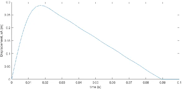
By running the model, the results for the displacement of node A, xA, can be consulted

in Figure 4.7. Where the maximum displacement was 0.285 m at 0.02 s, showing that the system was able to stop before reaching the maximum length available of 0.3 m. After that peak, the figure shows that the actuator rod starts to come back to his initial position where it is reached at 0.09 s.

Figure 4.7 - Displacement of node A obtained in the developed Matlab Simulink model.

From Figure 4.8, the velocity of node A, vA, shows that the actuator rod starts at 30 m/s

and slows down till 0 m/s in 0.02 s, where it represents the maximum displacement reached shown in the previous figure. The negative values from the graph represent the velocity during the opposite movement until the initial position under 0.09 s where that maximum velocity was always under 4.6 m/s.

Figure 4.8 - Velocity of node A obtained in the developed Matlab Simulink model.

The angle produced by the transmission lever can be seen in Figure 4.9, at the maximum displacement of the transmission lever it made a rotation of 28°. To have a more stable system and reduce the overall inclination of the lever the idea was to put the transmission lever at 76°

(46)

and then the system would make the 28° of movement so the transmission lever would be at 90° at the intermediate position. This means the lever system would move between 76° up to 104°.

Figure 4.9 - Angle produced by the transmission lever during its movement.

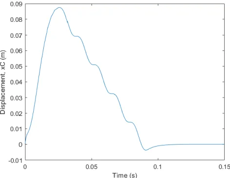
At the other end of the transmission lever would be connected to the springs and shock absorbers assembly. Figure 4.10 shows the displacement of node C, the contact point between the springs and shock absorbers assembly. The maximum displacement obtained was at 0.02 s meaning that it is the position where the lever system reaches the maximum angle produced, and the value is 0.085 m. After that, there is a “stairs” effect on the variation of the position of node C where it can be explained by the tension being released from the springs that after the compression they suffer and finally gets to the initial position under 0.15 s.

(47)

In Figure 4.11, the velocity of node C, vC, reaches a maximum velocity of 5.5 m/s at

0.01 s and quickly drops again to 0 m/s. At the start of the graph, there is an oscillation till it reaches the maximum velocity provoked by a transitory adaptation. After that, the velocity oscillates between 0 m/s and 2.8 m/s negative because it shows that the shock absorbers are going back to their initial position and that wave behavior is explained by the springs releasing tension. It was important to have a maximum velocity of around 5 m/s, since it is the maximum velocity that the shock absorbers were able to operate. The time of being over those 5 m/s was so short, less than 0.01 s, so it was considered that the system respected the limits of the shock absorbers.

Figure 4.11 - Velocity of node C obtained in the developed Matlab Simulink model.

4.2. Transmission lever

As it was previously said in the last chapter, to stop the actuator’s rod movement it was required a lever system to reduce the 30 m/s of velocity from the actuator’s rod to 5 m/s, were the industrial shock absorber and the spring could act and finally stop the movement of the rod. As such the initial task was to simulate with help of SolidWorks 2019 the forces that this lever system would have to operate to dimension the bars. Therefore, the designed transmission lever structure needs to be strong enough to withstand the impact load of the rod.

The final concept was to use two UPN120 standard profiles and reinforce them with C60 steel plates on the beams, that would be welded to the UPN profiles, as well as two tubular C45 steel, that would also be welded to the UPN profiles and connected together. The tubular steel on the bottom is used as well for the axle of this lever system, where the ratio of 3:1 is respected. On the bottom part of this transmission lever, there are two aluminium 7075-T6 plates, one on each side of the profiles, to allow the implementation of the skate, which will be presented in the next chapter. Therefore, the contact between the transmission lever and the spring could happen. These aluminium plates would be screwed to the UPN profiles. On the top part of the transmission lever there are two blocks of aluminium 7075-T6, one on each of the UPN profiles, also screwed, to receive the impact from the actuator. The final transmission lever assembly is represented in Figure 4.12, and all the mechanical drawings can be seen in Appendix C.

(48)

Figure 4.12 – Final model of the Transmission lever.

To start the simulation, it was required to determine the forces that this transmission lever would have to withstand. From the simulations run in Matlab Simulink, it was determined that on the bottom of the lever. The force was around 198 kN, the resultant force produced by the spring on node B, Fm, where the aluminium plate is allocated. This value can be consulted

in Appendix A, but at the time this study was being made the force used in SolidWorks simulation was calculated numerically.

From the kinetic energy produced by the actuator, it was possible to determine the energy of the rod’s motion and to verify that the energy is constant throughout the length of the transmission lever. It was made a rough estimate, so it was considered more mass than the actual mass used in Matlab Simulink simulation, 20 kg, and the velocity of 30 m/s.

𝐸 = 1 2 𝑚 ∗ 𝑣 2 E = 1 2 20 ∗ 30 2_{= 9000 J} (4.14)

Now, the energy provided from the actuator’s rod movement can be considered as equal to the elastic potential energy of the spring and since it is known the distanced stretched, x, from the Matlab Simulink simulation, the value of the spring constant k can be determined:

𝐸𝑃 = 1 2 𝑘 ∗ 𝑥 2 9000 = 1 2 𝑘 ∗ 0.08737 2_{ k = 2.35*10}6_N/m (4.15)

(49)

After obtaining the value of the spring constant, the force of the spring can be determined by:

𝐹 = 𝑘 ∗ 𝑥

F = 2.35*106 * 0.08737 = 206 kN (4.16)

The value of the force obtained by the equations was 206 kN so in the SolidWorks simulation, the force was approximated to 210 kN. That force was applied in the aluminium plate on the bottom of the transmission lever on the area where the skate would be screwed to the plate. This skate is a contact component between the transmission lever to the spring assembly, that will be explained in the next chapter. The structure would rotate on the axle of the transmission lever with a diameter of 60 mm. To simulate the slip contact between the stopping car and the transmission lever on the top it was used a cylindrical shaft in AISI 4340 steel. The diameter of this shaft is smaller than the area of contact between the aluminium blocks and the actuator, in this case, more critical results can occur. The mesh utilized in this simulation was a high mesh quality, the maximum allowed in SolidWorks2019’s software.

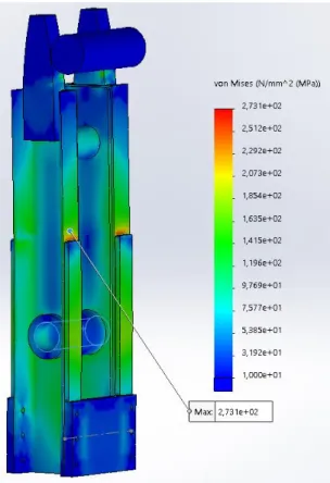
Inserting these values in SolidWorks 2019’s simulation parameters, it is possible to obtain the Von Mises stress distribution, shown in Figure 4.13. The maximum value found for the stress distribution was 273.1 MPa located in the small red area on the top of the beam’s reinforcements. No matter the length of the beam’s reinforcements, this behavior will always occur because of the indent between the parts since they have a clean edge. All the rest of the structure is way far from the yield strength of each of the materials utilized in the simulation.

Figure 4.13 - Von Mises stress distribution obtained when a 210 kN force is applied to the transmission lever structure, recurring SolidWorks 2019.

(50)

It was also possible to obtain the results for the factor of safety, shown in Figure 4.14. The minimum value found was 1, once again happening in the same where the Von Mises stress values were higher, but all the red areas represent all the values found under a factor of safety of 2.

Figure 4.14 - Factor of safety obtained when a 210 kN force is applied to the transmission lever, recurring to SolidWorks 2019.

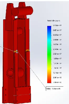
To make sure the structure was holding its integrity it was also made a fatigue test, shown in Figure 4.15, to determine the total life cycle. The minimum value obtained was 706400 cycles.

Figure 4.15 - Total life (cycle) obtained when a 210 kN force is applied to the transmission lever, recurring to SolidWorks 2019.

(51)

To connect all the parts that assemble the transmission lever, the fasteners are presented in Table 4.2.

Table 4.2 - Fasteners used to assemble the transmission lever.

Element Norm Qt.

Screws ISO 4762 M12x30 - 8.8 12

ISO 4762 M12x70 - 8.8 12

4.3. Skate

A mechanism to promote the contact between the transmission lever to the spring and shock absorber assembly was developed. The solution found was to build a skate, Figure 4.16, that would be supported by two plain bearings with a cylindrical shaft inside, where this shaft would be held by two bearings that would be screwed to the Aluminium plate of the transmission lever. This would give the ability of free rotation of the skate to enter in perfect contact to the spring during the rotation of the transmission lever and take the very high 210 kN force, with low contact pressures both on the skate surface and the plain bearings. All the mechanical parts drawings can be seen in Appendix C.

Figure 4.16 – Final model of the Skate.

(52)

Figure 4.17 - Transmission lever with the skate.

To start dimensioning this assembly, a simulation in SolidWorks 2019 was made, where it was applied the force of 210 kN, mentioned before, in the plate that would hold the springs assembly. It was possible to obtain the results of contact pressure in the skate’s surface, shown in Figure 4.18, to dimension the surface area of the skate. The goal was to get a surface tension under 70 MPa. The maximum value found was 444.9 MPa, but it was just a single node, so it was selected different nodes and all the values were under the 70 MPa of surface tension. All the materials used were C45 steel.

Figure 4.18 - Contact pressure obtained when a 210 k𝑁 force is applied to the Skate, recurring to SolidWorks 2019.

(53)

It was also made a Von Mises stress simulation, shown in Figure 4.19. This figure only shows the bearing, since it was the most critical part of the assembly, and the maximum value found was 529.8 MPa in a single node due to the mesh size. But it was impossible to refine more the mesh since it was the highest mesh quality possible in the software. To check the integrity of the components various nodes were selected around that critical value found and the results were much lower, around 380 MPa, and lower close to 126 MPa. Since the material selected, C45 steel has a yield strength of 580 MPa, it was considered that the component would keep its integrity with the impacts.

Figure 4.19 – Von Mises stress distribution obtained when a 210 k𝑁 force is applied to the Skate structure, recurring SolidWorks 2019.

To check the deflection of the cylindrical shaft it was also made a factor of safety test, where the minimum value found was 1.1 and the red areas represent the values under a factor of safety of 2.

Figure 4.20 – Factor of safety distribution obtained when a 210 k𝑁 force is applied to the Skate structure, recurring SolidWorks 2019.

(54)

The two plain bearings used in this assembly are EGB4030-E40 from Schaeffler [33] and the most important specifications are shown in. The use of two was required since each one could only withstand 168 kN.

Figure 4.21 - Plain bearing EGB4030-E40 specifications [33].

To connect all the parts and assemble the skate to the transmission lever, the materials are presented in

Table 4.3.

Table 4.3 - Fasteners used to connect all parts and assemble the skate to the transmission lever.

Element Norm Qt.

Screws ISO 4762 M8*50 - 8.8 4

Circlip DIN 471 - 38 x1.75 2

4.4. Spring

There were a lot of studies to find a solution for the spring to be used. Since this system would have to withstand big load forces, around 210 kN, a very strong spring would have to be found. The solution found was to use a stack of disc springs. The final model for this assembly is shown in Figure 4.22. The assembly is composed of two S890QL (1.8983) steel plates that will hold the disc springs combination. Those will be guided by two 40 mm diameter heat-treated H6 tubular shaft steel from Bosch Rexroth [15] with an inside diameter of 26.5 mm. The disc springs would be aligned with an Aluminium hollow shaft that would be threaded to one of the plates and aligned with the second one by a PTFE gasket.

(55)

Disc springs, or Belleville springs, are well known for their versatile assemble with a relatively small size, which allows them to have a wide range of applications with the desired load conditions.

When stacked in parallel the total deflection is equal to a deflection of a single disc spring and the total load capacity equals the load capacity for each spring times the number of springs in a stack. When put in series the total deflection equals the deflection of a single disc spring times the number of springs in a stack and the total load capacity is equal to a single disc spring load capacity. When assembled in parallel-series combinations they can be designed to accommodate virtually any load or deflection and to obtain progressive or regressive characteristics [34]. These combinations can also be explained in Figure 4.23.

Figure 4.23 - Explanation of the disc spring's combinations.

Since these combinations can obtain progressive, regressive, or linear characteristics with the use of flats or spacers between the stacks of disc springs, the solution found was to have a linear characteristic. This means that spring load increases progressively as the deflection increases. These different characteristics are represented in Figure 4.24.