1
Copyright © 2011 Cognizant Comm. Corp. www.cognizantcommunication.com
DETERMINANTS OF LENGTH OF STAY: A PARAMETRIC SURVIVAL
ANALYSIS
ANTÓNIO GOMES DE MENEZES and ANA MONIZ
Department of Economics and Management, University of the Azores, Ponta Delgada, Portugal
Length of stay is one of the most important decisions made by tourists as it conditions their overall expenditure and stress caused on local resources. This article estimates survival analysis models to learn the determinants of length of stay as survival analysis naturally lends itself to study the time elapsed between arrival and departure. It is found that sociodemographic profiles, such as nationality and gender, and trip attributes, such as repeat behavior, travel motive, and type of flight, are impor-tant determinants of length of stay. This article’s results are imporimpor-tant to design marketing strategies that effectively influence length of stay.
Key words: Length of stay; Survival analysis; Tourism demand modeling
Address correspondence to António Gomes de Menezes, Department of Economics and Management, University of the Azores, Rua da Máe de Deus, 9501-801 Ponta Delgada, Portugal. Tel: +351-296650084; Fax: +351-296650083; E-mail: [email protected]
Introduction
Length of stay is an important determinant of the overall impact of tourism in a given economy. The number of days that tourists stay at a particular des-tination is likely to influence their expenditure, for instance, as the number of possible experiences to be undertaken by tourists depends on their length of stay (Davies & Mangan, 1992; Kozak, 2004; Lego-herel, 1998). Understanding the determinants of length of stay is, thus, important to fully character-ize tourism demand and its impact on a given tour-ist destination (Gokovali, Bahar, & Kozak, 2007). In addition, Alegre and Pou (2006) argue that the importance of uncovering the determinants of length of stay and concomitant gains to policy makers and
researchers alike has grown with the increasingly pervasive pattern of shorter lengths of stays. Alegre and Pou claim that uncovering the microeconomic determinants of length of stay is critical to the de-sign of marketing policies that effectively promote longer stays, associated with higher occupancy rates and revenue streams. In fact, income from tourism might well be falling in many destinations despite the increase in visitor arrivals, due to a de-crease in the length of stay. Length of stay has also aroused interest beyond its importance as an expen-diture determinant. For instance, in the tourism sus-tainability literature, length of stay is important in the context of carrying capacity analysis (Saarinen, 2006). However, and as Gokovali et al. (2007) ar-gue, there are relatively few studies that estimate
the determinants of length of stay resorting to mi-croeconometric techniques. This article contributes to fill this gap.
The aim of this article is twofold. Firstly and foremost, and at a conceptual level, this article aims to establish if survival analysis models are suitable to model tourists’ length of stay. As survival analy-sis models are well established in several fields of knowledge (Greene, 2000), on the one hand, and there is virtually no prior application of such mod-els to the tourism literature (Gokovali et al., 2007), on the other, there is clearly an obvious gain to the social sciences, in general, and to the tourism litera-ture, in particular, of such cross-fertilization and inquiry. Secondly, this article aims to estimate the determinants of length of stay, in particular, how different individual sociodemographic profiles and trip experiences influence length of stay. By doing so, this article contributes to the social sciences by applying in a novel fashion survival analysis mod-els to research agendas that draw on marketing seg-mentation (see Kotler, 2001 for an introduction) and decision making theories (see Decrop & Snelders, 2004, and references therein).
Length of stay is one of the questions resolved by tourists when planning or while taking their trips (Decrop & Snelders, 2004). Hence, it follows that length of stay is best recorded when tourists depart, and, quite likely, is influenced by tourists’ socio dem-ographic profiles, on the one hand, and their experi-ences while visiting their destination, on the other (Bargeman & Poel, 2006; Decrop & Snelders, 2004). This article accounts for such insights by employ-ing micro data, rich on individual sociodemograph-ic characteristsociodemograph-ics and actual trip experiences, built from individual surveys answered by a representa-tive sample of tourists departing from the Azores: the Portuguese tourist region with the highest growth rate in the last decade.
Modeling length of stay poses certain challenges that owe to the fact that length of stay is, necessar-ily, a nonnegative variable. To uncover causal rela-tionships between tourists’ sociodemographic char-acteristics and trip experiences and length of stay, the empirical work must employ some sort of a for-mal statistical model. However, the most popular statistical tools, such as the linear regression model, are not appropriate to model length of stay, because they do not take into account that length of stay is a
nonnegative variable, and, hence, lead to biased es-timation (see Greene, 2000, for details). To circum-vent such problem, this article employs survival analysis parametric models in a novel way. This ar-ticle argues that survival analysis, or time to event analysis (read, departure), naturally lends itself to the study of length of stay. Quite interestingly, this article employs a plethora of survival analysis para-metric models that display much welcomed features. First and foremost, the survival analysis parametric models accommodate for individual heterogeneity, in the sense that a large number of covariates, per-taining to individual sociodemographic profiles and actual trip experiences, are used to explain length of stay, as suggested by microeconomic theory and a reading of the literature (Decrop & Snelders, 2004). Second, the survival analysis parametric models employed are unrestricted in the sense that they allow for nonnormal data patterns, such as spiky or bimodal data. This is especially important because some lengths of stays are more frequently found in the data than others, such as 7-day stays.
Recently, and not surprisingly, several authors have employed microeconometric models to ana-lyze the determinants of length of stay that explic-itly deal with the limited nature of length of stay, namely, being a nonnegative variable. Alegre and Pou (2006) employ a limited dependent variable discrete choice model, namely, a binary logit, and, thus, collapse length of stay into a binary variable: zero if length of stay is shorter than 1 week; one if otherwise. By doing so, the ensuing policy implica-tions are less far reaching, in the sense that all length of stays, say, shorter than 1 week are treated alike, be them 1-day stays or 6-day stays. This loss of information may be particularly worrisome when length of stays are not obviously dichotomized or clustered, and are, instead, roughly evenly distrib-uted over several days, leaving the researcher with no obvious cut-off to arbitrarily partition length of stays. To avoid this problem, Gokovali et al. (2007), like this article, employ survival analysis paramet-ric models to estimate the determinants of length of stay for a sample of tourists departing from a Turk-ish tourist region. While innovative and informa-tive, the work by Gokovali et al. (2007) is restricted to models of the Proportional Hazards form, and, therefore, with constant or monotone hazard rates: intuitively, the rate at which stays are terminated.
This article capitalizes on Gokovali et al. (2007) yet employs a more general and, concomitantly, richer approach. In particular, this article employs models not only of the Proportional Hazards form, as in Gokovali et al. (2007), but also of the Accelerated Failure-Time form, with the former being a special, nested case of the latter. This distinction matters because, and in a nutshell, the Proportional Hazards models, by construction, exhibit constant or mono-tone hazard rates. The Accelerated Failure-Time models, however, display no such restriction, and, hence, accommodate more general data patterns. This distinguishing feature is especially important in the present context because length of stays may exhibit spiky, multimodal patterns, depending on the destination or the time period under analysis. Therefore, this article’s framework is applicable to any kind of tourism destination. It should also be noted that this article’s approach leads, ex ante, to models with a better fit to the data. In fact, the Pro-portional Hazards models are, in a formal statistical sense, nested cases of Accelerated Failure-Time models, and this article employs a model selection strategy—estimating both Proportional Hazards models and Accelerated-Failure-Time models— that clearly dominates a model selection strategy that estimates only the special case Proportional Hazards model. This turns out to be case, as ex-pected. In fact, the econometric work carried out in this article selects an Accelerated Failure-Time model as the preferred model, despite the fact that the Proportional Hazards models do display quite satisfactory statistical results.
The theoretical framework underlying this arti-cle draws from two strands of the social sciences literature. First, and quite naturally, this article draws heavily on the literature on marketing seg-mentation. Segmentation is a methodological pro-cess of dividing a market into distinct groups that might require separate experiences or marketing service mixes (Venugopal & Baets, 1994). Segmen-tation includes the identification and assessment of various tourist characteristics (such as demograph-ics, socioeconomic factors, and geographic loca-tion) and product-related behavior characteristics (such as purchase behavior, consumption behavior, and attitudes towards and preference for attrac-tions, experiences, and services). Target marketing is a strategy that aims at grouping a destination’s
markets into segments so as to aim at one or more of these by developing products and marketing pro-grams tailored to each (Kotler, 2001). The need for in-depth knowledge of segments remains an essen-tial element of understanding the homogeneous be-havior of groups of tourists. Market segmentation in tourism techniques rangees from elementary per-centiles and quartiles to more complex multivariate techniques such as factor analysis, principle compo-nents, cluster analysis, and neural networks (Bloom, 2005; Galloway, 2002; Jang, Morrison, & O’Leary, 2002; Mok & Iverson, 2000). Hence, this article contributes to the market segmentation literature with a novel exercise that shows that survival anal-ysis is a powerful and informative tool to be used by marketing strategists. More interestingly, this articles’ unrestricted approach to the data makes it suitable to a variety of contexts in the social sciences.
Second, this article draws on decision-making theories, including microeconomic theory, as they motivate empirical work on the microdeterminants of length of stay, resorting to econometric tech-niques. As Alegre and Pou (2006) discuss, discrete choice models as proposed by Dubin and McFad-den (1984), Hanemann (1984), and Pollak (1969, 1971) provide a framework that allows one to write the conditional demand function for the length of stay at a given destination, and assuming weak sep-arability between the tourist trip and consumer goods other than tourism, as a function of holiday charac-teristics, the daily price of the holiday, the total ex-penditure available for the holiday, maximum time available, the characteristics of the tourist, and a nonobservable random effect. On the other hand, and as Hellström (2006) surveys, several authors have recently proposed in the recreational demand literature consumer choice models that endoge-nously determine time on-site (Berman & Kim, 1999; Feather & Shaw, 1999; Hellström, 2006; Larson, 1993; McConnell, 1992). In its essence, the aim of this research program is to solve the prob-lem of a utility maximizing consumer whose choic-es of number of trips per period may be jointly and endogenously determined with the number of nights per trip, in a setting suitable for welfare analysis, that explicitly addresses the unavoidable data prob-lems associated with the integer nature of length of stay (see Hellström, 2006, for a theoretical and em-pirical illustration along these lines; see
Papathe-odorou, 2001, for a critical review of consumer theory in a destination choice context). In addition, the specification of the regressions found in this ar-ticle’s econometric work draws on consumer be-havior models that suggest the factors to include as determinants of length of stay (see Jafari, 1987; Mathieson & Wall, 1992; Moscardo, Morrison, Pearce, Lang, & O’Leary, 1996; Swarbrooke & Horner, 2001 and references therein, for discus-sions on models of consumer behavior).
The empirical work carried out in this article produced statistically significant and economically important results. Several sociodemographic indi-vidual characteristics and trip attributes turn out to be statistically important determinants of length of stay, and, carry, thus, important policy implica-tions. In fact, the results uncovered may be used to aid the design of marketing policies that may pro-mote longer stays. In addition, there are results that shed light on enduring research topics, such as re-peat visitor behavior. In fact, it should be noted that repeat visitors display higher probabilities of expe-riencing longer stays, a fact in line with the findings in Lehto, O’Leary, and Morrison (2004), who claim that repeat visitors exhibit extended length of stays.
Determinants of Length of Stay: A Parametric Survival Analysis
Length of stay is one of the most useful dimsions used to characterize tourism demand: an en-during research topic (for extensive reviews of re-search on tourism demand see, among others, Crouch, 1994; Crouch & Louviére, 2000; Lim, 1997; Song & Witt, 2000; Witt & Witt, 1995). Tourism demand is a broadly defined subject that encompasses a va-riety of objects, interesting in their own right: tour-ist arrivals, tourtour-ist expenditure, travel exports, nights spent in tourist accommodations, and length of stay. Length of stay is an interesting research topic for, at least, two reasons. First, length of stay conditions the overall socioeconomic impact of tourism in a given economy. In fact, and as Davies and Mangan (1992) and Kozak (2004), among oth-ers, argue, an increased length of stay may allow tourists to undertake a larger number of experienc-es or activitiexperienc-es that may affect their overall spend-ing and sense of affiliation. Hence, several authors consider length of stay an important market
seg-mentation variable in estimating the determinants of tourist spending (Davies & Mangan, 1992; Leg-oherel, 1998; Mok & Iverson, 2000). Second, mod-eling length of stay is important to tourism sustain-ability analysis (Saarinen, 2006). Sustainsustain-ability has recently become an important policy issue in tour-ism. The ubiquitous continuous growth of tourism has fueled an intense discussion about the socio-economic and environmental impacts that tourism hinges on destination areas. In the sustainability lit-erature, an important concern focuses on destina-tion areas’ carrying capacity, generally defined as the maximum number of people who can use a site without any unacceptable alteration in the physical environment and without any unacceptable decline in the quality of the experience gained by tourists. The concept of carrying capacity occupies a key position with regard to sustainable tourism, in that many of the latter’s principles are based on this theory and research tradition. Models of the deter-minants of length of stay are important to the re-search on sustainable tourism because they are useful to forecast tourists’ on-site time, and, con-comitantly, the stress caused by tourism activity on local resources.
Despite the rich literature on tourism demand, Alegre and Pou (2006) argue that most studies on tourism demand fail to pay attention to length of stay, at least at a microeconometric level, where one is able to control for individual heterogeneous behavior. Moreover, the few studies available in the literature on the length of stay are mainly de-scriptive (Oppermannn, 1995, 1997; Seaton & Palm-er, 1997; Sung, Morrison, Hong, & Leary, 2001). These studies show how length of stay varies with nationality, age, occupation status, repeat visit be-havior, stage in the family life cycle, and physical distance between place of origin and destination, among other variables. While these studies do find interesting results, their descriptive nature hinders formal inference tests on the causal relationships between individual sociodemographic profiles and actual trip experiences and length of stay. Recently, however, some authors have employed micro-econometric models to estimate the determinants of length of stay. Fleischer and Pizam (2002) employ a Tobit model to estimate the determinants of the vacation-taking decision process for a group of Is-raeli senior citizens. The Tobit model in Fleischer
and Pizam (2002) overcomes the fact that several individuals in the study group do not take vacations at all, and, thus, the model allows a corner solution case, with many individuals experiencing zero days of vacation. Fleischer and Pizam (2002) conclude that age, health status, and income have a positive effect on the length of stay. In the present case, only departing tourists were surveyed, and, hence, all tourists experienced a strictly positive length of stay. Therefore, the Tobit model, employed in Fleischer and Pizam (2002), is not applicable. Alegre and Pou (2006) analyze length of stay for a pooled cross-section of tourists visiting the Balearic Islands. Alegre and Pou (2006) employ a logit model, where the explanatory variable is binary (0 if length of stay is shorter than one week and 1 otherwise), and find, among other results, that labor status, nation-ality, and repeat visitation rate are statistically sig-nificant determinants of length of stay. Gokovali et al. (2007) estimate parametric survival analysis models of the Proportional Hazards form to learn that, for a cross section of tourists departing from the Turkish region of Bodrum, a seasoned tourist (i.e., someone who has traveled as a tourist exten-sively), past visits to destination, overall attractive-ness, and image of destination country, all increase the probability of staying longer.
Contextual Setting
The Azores are a Portuguese archipelago, with nine islands, a population of 242,000 inhabitants, and an autonomous government. The Azores, with their strikingly beautiful nature, are the Portuguese region where tourism has grown more rapidly in the last decade. Tourists’ nights spent in tourist ac-commodations increased from 407,000 in 1995 to over 1,200,000 in 2006. Despite the obvious tourist growth potential, until the early 1990s tourism was not promoted by the regional government. In the mid-1990s, a change in the regional government led to a change in tourism policy, which led to a boom in hotel construction, with the total number of hotels beds growing from 3,000 in 1995 to 10,000 in 2005 (data source: SREA statistical of-fice; http://srea.ine.pt).
Despite the recent successes, several challenges remain. Ranking high among the most pressing is-sues one finds a desire by public officials and hotel
operators to increase average length of stay, which is perceived as critical to increase occupancy rates and make operations smoother to run. Hence, learning the determinants of length of stay is critical to im-prove the effectiveness of regional tourism policy.
Study Methods
Survey Design and Data Collection
The research proceeded in two stages. In the first stage, a questionnaire was designed and tested us-ing a control group of 50 tourists in the sprus-ing of 2003. The questionnaire was used to construct the data set employed in the empirical part of the arti-cle and was carried out in the summer of 2003, in the second stage of the research. The questionnaire was built as a representative, stratified sample of the tourists who visited the Azores, by nationality, routes, and gateways used, in the year of 2002. The total number of respondents—400—was determined according to the methods discussed in Hill and Hill (2002). In the summer of 2003 there were three gateways—Ponta Delgada, Lajes, Horta—, in the three main islands of São Miguel, Terceira, and Faial, respectively. The questionnaires were carried out at these airports, near the boarding gates, in three languages: Portuguese, English, and Swedish. The questionnaires were applied through personal interviews, with the interviewers possessing formal instruction on the matter.
The questionnaires were developed as to be able to test the following hypotheses, as discussed in the introduction and the literature section above, herein stated in a succinct form:
H1: Individual sociodemographic profiles influ-ence length of stay.
H2: Individual actual travel experiences and atti-tudes influence length of stay.
Hence, each questionnaire covered individual sociodemographic profiles, by including variables such as gender, age, education, occupation sector, type of profession, marital status, among others, which allow a thorough test of H1. By the same token, each questionnaire covered actual trip expe-riences, by including variables such as travel party composition, travel motive, motives underlying destination choice, alternative destinations consid-ered, repeat visitation rate, tourist experience,
over-all satisfaction, revisit intention, among others, in order to test H2.
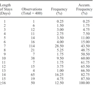
Table 1 lists the highest frequencies of length of stay. As expected, the highest frequency is 7-day stays, typically associated with tourists visiting on tour operator packages, with an in-sample frequen-cy of 28%. The combined frequenfrequen-cy of 14–15-day stays is also quite high: about 20%. About half of the stays last no longer than 8 days.
Table 2 contains additional selected, self-explan-atory, descriptive statistics for the data gathered.
Overall, mean stay is about 11 days; median stay is just 10 days while the standard deviation of stays is about 11 days, due to some quite long stays. The largest group of tourists in the sample is tourists from Mainland Portugal, who experience stays similar to those of the overall sample and are the youngest group. Tourists from the Nordic Countries (namely, Norway, Finland, and Denmark)1 are the second largest group in the sample and exhibit a mean stay of 9 days, a median stay of 7 days, and a relatively low standard deviation of 3 days, as most of these tourists visit with either 1- or 2-week tour packages. (We treat Sweden separately because of its remark-able importance as an origin country for the Azorean tourism as a whole.) Tourists from Germany experi-ence, typically, longer stays than tourists from the Nordic Countries. In sum, there are interesting dif-ferences in length of stays across nationalities.
Survival Analysis
Survival analysis is just another name for time to event analysis. The engineering sciences have con-tributed to the development of survival analysis, which is called “reliability analysis’’ because the main focus is in modeling the time it takes for ma-chines to break down. Likewise, survival analysis has long been a cornerstone of biomedical research. The analysis of duration data comes fairly recently to the social science literature, arguably with a more significant impact on applied economics lit-erature (for applications of survival analysis in eco-nomics, see, among others, Cleves, Gould, & Guti-errez 2002; Greene, 2000; Hosmer & Lemeshow, 1999; Kieffer, 1988; Lancaster, 1990).
This framework of analysis naturally lends itself to the study of length of stay, as one is interested in the determinants of the length of time that elapses between the tourist’s arrival on a given tourist des-tination and his departure. The data set employed in the present article was collected at airports from tourists who were departing from their trips. Hence, there is no censoring in the data because all inter-viewees reported their length of stay. Therefore, the discussion that follows assumes away censoring.
Spell length is, by construction, a nonnegative variable. Let spell length be represented by a ran-dom variable T, with continuous probability distri-bution f(t), where t is a realization of T. It is usually the case that one is interested in the probability that the spell is of length at least t, which is given by the survival function S(t) = P(T ≥ t). The hazard rate, λ(t), in turn, answers the following question: Given that the spell has lasted until time t, what is the probability that it will end in the next short interval of time, Δ? More formally:
λ( ) lim ( | ) ( ) ( ) t P t T t T t f t S t = ≤ ≤ + ≥ = > ∆ ∆ ∆ 0 (1)
Intuitively, the hazard rate is the rate at which spells are completed after duration t, given that they last at least until t. Armed with the hazard rate, one computes the survival function through backward integration. Hence, and as a matter of convenience, one usually focuses on estimating the hazard func-tion directly.
Two frequently used models for adjusting
sur-Table 1
Distribution of Length of Stays
Length of Stays
(Days) Observations (Total = 400) Frequency (%)
Accum. Frequency (%) 1 1 0.25 0.25 2 6 1.50 1.75 3 12 3.00 4.75 4 11 2.75 7.50 5 14 3.50 11.00 6 16 4.00 15.00 7 114 28.50 43.50 8 21 5.25 48.75 9 7 1.75 50.50 10 38 9.50 60.00 11 7 1.75 61.75 12 15 3.75 65.50 13 4 1.00 66.50 14 65 16.25 82.75 15 19 4.75 87.50 ≥16 50 12.50 100.00
vival functions for the effects of covariates are the Accelerated Failure-Time (AFT) model and the multiplicative or Proportional hazards (PH) model (Green, 2000). In the AFT model, the natural loga-rithm of the survival time lnT, is expressed as a lin-ear function of the (1*k) vector of time-invariant covariates x, yielding the linear model lnt = xβ + z, where β is a (k*1) vector of regression coefficients to be estimated, and z is the error term with density
f(). The distributional form of the error term
deter-mines the regression model.
In the proportional hazards model, the concomi-tant covariates have a multiplicative effect on the hazard function:
λ(t,xi) = λ0(t)exp(xiβ)
(2) where λ0(t) is the baseline hazard function. Intui-tively, the baseline hazard function λ0(t) summa-rizes the pattern of duration dependence and is common to all persons while exp(xiβ) is a nonnega-tive function of person-specific covariates xi, which scales the baseline hazard function common to all persons, controlling, hence, the effect of individual heterogeneity.
The PH property implies that absolute
differ-ences in x imply proportionate differdiffer-ences in the hazard rate at each t. For some t = t, and for two persons i and j identical in all matters except with respect to the kth covariate, then a unit increase in the kth covariate induces the following proportion-ate change in the hazard rproportion-ates:
λ λ β ( , ) ( , ) exp( ) t x t x i j k = (3)
The above expression lends a natural interpretation to Βk, namely, the log hazard ratio βk = ∂logλ(t,x)/∂ logxk, which is easily recognized as either a semi-elasticity or semi-elasticity.
The baseline function may be left unspecified, yielding the semiparametric Cox PH model, or it may take a specific parametric distributional form, which, and assuming that the correct distributional form is chosen, leads to more efficient estimates.
The choice of a particular distribution matters because it conditions the slope of the hazard func-tion. A particular distribution yields a particular hazard function, which may feature duration de-pendence, in the sense that the probability that ter-mination of a stay occurs in the next short interval
Table 2
Selected Descriptive Statistics
Variables Observations Frequency(%) Average Stay(Days) Median Stay(Days) SD Stay(Days) Age (Years)Average Sociodemographic profiles
Portugal (Mainland) 150 37.50 11 10 11 34
Sweden 95 23.75 9 7 3 57
Other Nordic countries 49 12.25 9 7 3 47
Germany 21 5.25 14 8 24 41
Other countries 85 21.25 17 14 14 44
Male 203 50.75 11 8 11 44
Marital status (married) 264 66.00 11.8 9.5 12 49
Azorean ascendancy 70 17.50 18.7 15 13.2 43
Education1. Secondary 127 31.75 10.9 10 6.8 40
Education2. Tertiary 183 45.75 10.6 7 10.3 45
Education3. Technical 8 2.00 8.6 7 3 48
Education4. Lesser 82 20.50 16.8 13 17 47
High level profession 127 31.75 10.2 8 6.5 48
Trip attributes Leisure 294 73.50 10.6 8 8.6 45 Visit friends/relatives 57 14.25 17.4 15 14 44 Business 35 8.75 15.6 10 22 36 Other motive 14 3.50 8.5 6 6.2 37 Repeat visitor 141 35.25 16.5 14 16.7 41 Charter flight 150 37.50 11.2 7 6.9 52 Total 400 100.00 11 9 11 43
of time may depend on length of stay. Because there is scant or virtual none empirical evidence on the shape of the hazard function of lengths of stays, this article takes an agnostic view and entertains the possibility of a myriad of shapes of the hazard function. Hence, the hazard function of stays is es-timated under the following six alternative distribu-tions—exponential, Weibull, Gompertz, the three most popular PH models (Green, 2000); general-ized gamma, lognormal and log-logistic, the most widely employed AFT models (Green, 2000)— which altogether accommodate, ex ante, several possible shapes of the hazard function. It should be noted that the above-mentioned semiparametric Cox model was also estimated and the results do not change in a meaningful manner from the results obtained under the parametric models, extensively discussed below. To save on space, the discussion that follows focuses on the parametric analysis, which, arguably, produces more efficient estimates.
The exponential distribution yields a constant hazard rate λ0(t) = λ and hence is suitable to model length of stay when the probability of termination of a stay in the next short interval of time does not depend on the length of the stay. The Weibull dis-tribution, in turn, is a generalization of the expo-nential distribution and is suitable for modeling data with monotone hazard rates that either increase or decrease exponentially with time. The corre-sponding baseline function is λ0(t) = pλt p–1, where
p is an ancillary parameter to be estimated from the
data. Note that when p = 1 the Weibull model col-lapses to the exponential model. The Gompertz dis-tribution yields the baseline function λ0(t) = exp(γt), where γ is an ancillary parameter to be estimated from the data. Like the Weibull distribution, the Gompertz distribution is suitable for modeling data with monotone hazard rates that either increase or decrease exponentially over time. Unlike the PH models—namely the exponential, Weibull, and Gompertz models—the lognormal and log-logistic are two AFT models that tend to produce similar results and are indicated for data exhibiting non-monotonic hazard rates, specifically initially in-creasing and then dein-creasing rates. Finally, the gen-eralized gamma, another AFT model, yields a hazard function extremely flexible, allowing for a large number of possible shapes, including as
spe-cial cases the Weibull, the exponential and the log-normal models.
To sum up, survival analysis is suitable when the researcher is interested in learning the determinants of the time it takes between two events (or end of observation). This article agnostic approach to the data—of estimating a variety of competing models and, concomitantly, of letting the data speak in or-der to choose the appropriate statistical model— makes it especially portable to other social sciences fields, whenever time length is recordable and of interest.
Model Estimation and Model Selection
Model estimation is done via maximum likeli-hood, given the parametric nature of the six com-peting models. With respect to model selection, a reasonable question to ask is: “Given that we have several possible parametric models, how can we select one?” When parametric models are nested, the likelihood ratio or Wald tests can be used to discriminate between them (Green, 2000). When models are not nested, however, these tests are in-appropriate and the task of discriminating between models becomes more difficult. A common ap-proach to this problem is to use the Akaike infor-mation criterion (AIC; see Green, 2000, inter alia), which, in its essence, penalizes the log likelihood of a given model to reflect the number of parame-ters estimated. The AIC is defined as [–2(log likeli-hood) + 2(c + p + 1)], where c is the number of model covariates and p is the number of model-specific ancillary parameters. Because the log like-lihood obtained for any given parametric model depends on the set of covariates used, the set of co-variates of interest is defined ex ante and then em-ployed in the estimation of all the six competing models. Overall, 31 covariates were selected given the available data, on the one hand, and a reading of the literature, on the other, and are described at length in the next section, while the rest of this sec-tion focuses on model selecsec-tion. Table 3 presents summary results of the log likelihood estimation, ancillary parameters, model discriminating Wald tests and AIC values. (We use statistics package software Stata v. 9.0 to estimate the models and de-rive the tests.)
The Weibull model dominates the exponential model in all criteria considered. The log likelihood obtained under the Weibull model is higher than the log likelihood obtained under the exponential model. A Wald test that p, the Weibull model ancil-lary parameter, is statistically equal to 1—the case when the Weibull model collapses into the expo-nential model—is firmly rejected. In addition, the AIC value obtained under the Weibull model is lower than the AIC value obtained under the expo-nential model. Hence, the expoexpo-nential model is not used elsewhere in this article, because it is domi-nated by the Weibull model. Note that p has a point estimate of 1.9027, which is indicative of an up-ward sloping monotone hazard rate.
Like the Weibull model, the Gompertz model is suitable for modeling data with monotone hazard rates that either increase or decrease exponentially over time. Although the Weibull model cannot be formally tested against the Gompertz model, it should be noted that the Weibull model yields a higher log likelihood and a lower AIC value than the Gompertz model. Hence, the Weibull model is preferred to the Gompertz model and is the pre-ferred PH model. Quite interestingly, the point esti-mate of γ, the ancillary parameter of the Gompertz model, is 0.0167, and, hence, the Gompertz’s mod-el associated hazard rate displays a monotone and increasing hazard rate: the same result obtained un-der the Weibull model.
The log-logistic model produces the lowest AIC value of all the six models considered. The log- logistic model also produces the highest log likeli-hood value among all the six competing models. The log-logistic model cannot be formally tested against the other models as it is a nonnested case. Hence, it is not possible to reject the idea that the log-logistic model produces the overall best fit to the data.
The lognormal model yields results similar to the log-logistic model, as expected. The generalized gamma model provides an array of discriminating Wald tests, as it nests the exponential model, the Weibull model, and the lognormal model. The gamma model dominates the exponential model: not only does the generalized gamma model yields a lower AIC value and a higher log likelihood but also the Wald test that (σ,κ) = (1,1) produces a p-value of 0.0000. It is also the case that the general-ized gamma model dominates the Weibull model. In fact, the generalized gamma model produces a lower AIC value than the Weibull model, and, based on a discriminating Wald test κ = 1, the Weibull model is strongly rejected as a special case of the generalized gamma model. When the generalized gamma model is compared against the lognormal model, the picture that emerges is not so clear. The lognormal model corresponds to the generalized gamma model in the special case κ = 0. The Wald test that κ = 0 yields a chi-square value of 2.93 and
Table 3 Model Selection
Model Statistics Nested Models Wald Tests AIC
Exponential (PH) LL = –455.90; χ2(31) 62.36, p = 0.0007 None 977.80
Weibull (PH) (p = 1.9027) LL = –346.28; χ2(31) = 211.48, p = 0.0000 H
0: p = 1→χ2(1) = 162,
p = 0.0000→Reject exponential 760.57 Gompertz (PH) (γ = 0.0167) LL = –445.17; χ2(31) = 83.68, p = 0.0000 None 958.34
Lognormal (AFT) (σ = 0.5177) LL = –304.23; χ2(31) = 131.68, p = 0.0000 None 676.47
Log-logistic (AFT) (γ = 0.2687) LL = –282.01; χ2(31) = 145.38, p = 0.0000 None 632.03
Generalized gamma (AFT)
(κ = –0.1843; σ = 0.5128) LL = –302.77; χ2(30) = 127.97, p = 0.0000 H0: κ = 1→χ
2(1) = 120, p = 0.0000;
Reject Weibull 675.54
H0: κ = 0→χ2(1) = 2.93, p = 0.0872;
Not Reject lognormal
H0: (σ,κ) = (1,1)→χ2(2) = 764.41,
associated p-value of 0.0872, and hence it is not possible to reject the lognormal model at the 10% significance level, because at this significance level the corresponding chi-square is 2.70. However, one can also argue in favor of the generalized gamma model because it produces a slightly lower AIC value than the lognormal model.
In conclusion, the Weibull model strictly domi-nates both the exponential and the Gompertz mod-el, and is kept in the analysis, as the preferred PH model, for comparison purposes. With respect to the AFT models considered, it should be noted that the log-logistic model produces not only the lowest AIC value but also the highest log likelihood of all six competing models, and cannot be formally test-ed against any other model as it is a nonnesttest-ed model. Because all the AFT models produce re-markably similar results, the regression coefficients of the AFT models are reported only for the log-logistic model, to save on space.
Results
Table 4 reports the results obtained from the Weibull model—the preferred PH model—and the log-logistic model—the preferred AFT model. It should be noted that the coefficients are not directly comparable across models. The Weibull model is presented in PH form and the coefficients may be interpreted as a hazard ratio. Intuitively, and focus-ing on binary variables, the coefficients presented are of the form exp(βκ) and represent the ratio be-tween the hazard rate when the variable takes the value of one and the hazard rate when the variable takes the value of zero. Hence, a coefficient higher than 1 means that an increase in the variable leads to an increase in the hazard rate, and, thus, to a low-er expected duration. In turn, the log-logistic model is presented in AFT form and a negative coefficient is associated with shorter expected time to termi-nation of a stay. Hence, and if one is interested in comparing the qualitative meaning of the coeffi-cients across models, then coefficoeffi-cients higher (low-er) than 1 in the Weibull model correspond to nega-tive (posinega-tive) coefficients in the log-logistic model. At a quantitative level, there may be differences in the results arising from the different model specifi-cations, including about the distribution of the er-rors. However, and quite importantly, it should be
noted that ex ante the research has no formal way of anticipating the differences across models. Hence, our approach is rather agnostic and we let the data speak by looking at both preferred models. We find that overall, and ex post, the results are rather simi-lar across models. Inspection of Table 4 reveals that, in fact, the Weibull model and the log-logistic model tend to produce the same results, at least at a qualitative level.
The age coefficients are not individually statisti-cally significant in both models. As Alegre and Pou (2006) suggest, this may owe to the inclusion of other covariates closely related with age.
Male tourists tend to experience shorter stays. This result is statistically significant for both the Weibull model and the log-logistic model. There is no clear effect for being married.
Tourists from the Nordic Countries, including Swedes, experience shorter stays. These results are statistically significant in both models and have portant policy implications given the strategic im-portance of these markets in the Azorean tourism context. The results for tourists from Mainland Por-tugal have no statistical significance in both mod-els. The regression results fail to uncover a statis-tically significant effect for German tourists, either positive or negative. This is interesting because, and according to the descriptive statistics found in Table 2, tourists of German nationality exhibit the highest mean length of stay among all nationalities considered. The lack of statistical significance of the German nationality dummy variable is indica-tive of how misleading descripindica-tive statistics may be to base inference and, concomitantly, of the impor-tance of including a large number of covariates per-taining to individual sociodemographic profiles and trip experiences. Overall, the regression coefficients on nationalities do not follow any clear pattern, at least not according to the physical distance between the tourists’ place of origin and destination. In fact,
ex ante one would imagine that tourists who live far
away would experience longer stays to make up for the increased overall travel cost. However, when one controls for sociodemographic profiles and trip attributes, it turns out that this pattern is not statisti-cally significant. This is indeed the present case. In particular, it is found that the binary variable char-ter that equals 1 if the tourist took a (often direct) charter flight (and zero otherwise) significantly
in-creases the length of stay. Considering that virtual-ly all tourists from the Nordic Countries took char-ter flights, it becomes less of a paradox that having a nationality from the Nordic Countries is associ-ated with shorter length of stays. The reverse could be said about tourists from Mainland Portugal. Once more, this remark highlights the importance of controlling for a significant number of covariates.
Azorean ascendancy is a binary variable that equals 1 in case the tourist claims to have some sort of Azorean ascendancy. The Azorean diaspora far outnumber the current Azorean population and there are many Azorean descendents, typically
re-siding in North America, who visit the Azores. It is found, in both models, that having an Azorean as-cendancy reduces expected time to termination of stays, a result highly statistically significant under the log-logistic model.
With respect to the education variables, it should be noted that the excluded class is an education class associated with a lesser degree of education. The education variables have no statistical signifi-cance in the log-logistic model. Hence, the picture that emerges is that education is not associated in a statistically significant manner with length of stay.
High level profession is a binary variable that
Table 4
Regression Results
Variables Weibull [PH Form; exp(β(LL = –346.28, N = 400)k)] Log-logistic (AFT Form) (LL = –282.01, N = 400) Age1: ≥25 and <35 years 0.9455 (–0.27)*** 0.0071 (0.08)***
Age2: ≥35 and <45 years 0.7867 (–0.98) –0.0252 (–0.23)***
Age3: ≥45 and <55 years 1.0353 (0.14)*** –0.0467 (–0.44)***
Age4: ≥55 years 0.8506 (–0.68) 0.0793 (0.74)***
Male 1.2605 (2.03)*** –0.0842 (–1.68)***
Married 1.4595 (2.18)*** –0.1111 (–1.51)***
Sweden 1.9116 (2.19)*** –0.2677 (–2.17)***
Other Nordic country 1.7013 (1.82)*** –0.2107 (–1.73)***
Germany 0.5761 (–1.77)*** –0.0777 (–0.64)*** Portugal (Mainland) 1.2630 (1.32)*** –0.1247 (–1.58)*** Azorean ascendancy 0.7774 (–1.11)*** 0.3047 (3.12)*** Education1: Secondary 1.6643 (2.86)*** –0.0424 (–0.56)*** Education2: Tertiary 1.6306 (2.69)*** –0.0987 (–1.24)*** Education3: Technical 2.6112 (1.93)*** –0.2090 (–1.05)***
High level profession 1.1833 (1.24)*** –0.0404 (–0.065)***
Motive1: Leisure 0.6305 (–1.62)*** 0.2462 (1.84)***
Motive2: Visiting friends or relatives 0.6117 (–1.40)*** 0.3541 (2.23)***
Motive3: Business 0.1864 (–4.49)*** 0.3242 (1.95)***
Repeat visitor 0.5223 (–3.80)*** 0.1427 (1.94)***
Considered alternative destination 0.8725 (–0.76)*** 0.0417 (0.55)*** Considered alternative island destination 1.009 (0.04)*** 0.0035 (0.03)*** Azorean circuit (island hopping) 0.8926 (–0.48)*** –0.1638 (–1.49)*** Number of islands visited 0.7576 (–2.46)*** 0.2129 (4.00)*** Travel party 1: With spouse 0.9566 (–0.22)*** 0.0262 (0.29)*** Travel party 2: With family 0.9834 (–0.08)*** 0.0774 (0.80)*** Travel party 3: With other adults 1.7882 (2.54)*** –0.1364 (–1.44)*** Travel party 4: With business partners 3.1914 (3.93)*** –0.1130 (–0.86)*** Not coming back off-season 0.8670 (–0.68)*** 0.1294 (1.46)*** Highly satisfied with visit 0.7290 (–2.58)*** 0.0538 (1.02)***
Intends to revisit 1.1069 (0.59)*** 0.0683 (0.93)***
Came in a charter flight 0.5023 (–2.71)*** 0.3249 (3.14)*** p ancillary parameter Weibull 1.9027***
γ ancillary parameter log-logistic 0.2687***
Values in parenthesis are t-stats; Weibull coefficients are hazard ratios; Log-logistic coefficients in AFT form.
*Significant at the 10% level. **Significant at the 5% level. ***Significant at the 1% level.
takes the value of 1 for professions associated with high incomes and high social status. In this sense, high level profession proxies top incomes. A first group of 50 tourists were interviewed in a first stage of the field work in order to validate the ques-tionnaire. From this validation exercise, it followed that not all tourists were willing to report directly their income, and, hence, such proxy for income, based on current professional status, was built in the questionnaire. In both models, high level pro-fession has no statistical significance.
Travel motive was divided into four classes: lei-sure; visiting friends or relatives; business, and, the excluded class, other motives (which includes, for instance, religious festivities). It is found that, com-pared to the excluded class, all travel motives ex-plicitly considered increase expected duration of stays, a result with high statistical significance in the log-logistic model. As Seaton and Palmer (1997) suggest, tourists visiting friends or relatives tend to exhibit longer stays if they are international tour-ists, as it is generally the case in the Azores.
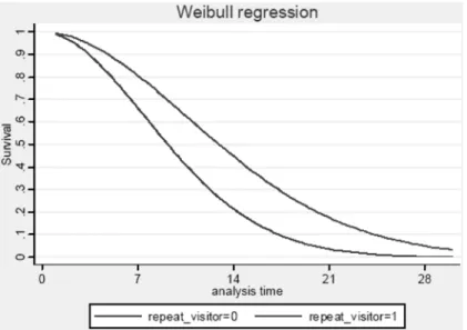
Repeat visitor is a binary variable that takes the value of 1 if the tourist visited the Azores at least once in the past, and zero otherwise. Quite interest-ingly, in both models it is found that repeat visitors stay for longer periods. In fact, everything else the same, being a repeat visitor reduces the hazard rate to half (0.5223) in the Weibull model. Repeat visi-tor behavior has aroused interest in the recent years (see, among others, Kozak, 2001; Lehto et al., 2004; Oppermann, 1997); its relationship with future vis-iting behavior (destination loyalty) and word-of-mouth recommendation carries important policy and marketing implications. It is interesting to note the strikingly different expected on-site time spent by repeaters from first-timers, as Figure 1 docu-ments. Figure 1 plots two survival functions, one for repeat visitors and one for first-time visitors. The survival function for repeat visitors is shifted to the right, which means that repeat visitors are associated with a higher probability of experienc-ing a stay of at least a given duration. For instance, the probability that repeaters stay for at least 14 days is about 45%, more than double the analogous probability for first-timers: about 20%.
Clearly, it would be trivial to plot other figures akin to Figure 1 for other segments, yet we refrain to do so for the sake of parsimony (other figures
available upon request). It should be noted that the figure is plotted evaluating the other attributes at their sample average and the distance between curves is capturing the repeat visitor effect. Differ-ent evaluations would shift both curves yet the main results would be left unchanged as there are no interactions between repeat visitor and other characteristics or segments in the model.
Considered alternative destination and consid-ered alternative island destination are two dummy variables that characterize the destination decision process. However, both variables are not statisti-cally significant in both models.
There are nine islands in the Azores. However, most tourists visit only one island: São Miguel, by far the largest and most populated one. Azorean cir-cuit is a binary variable that takes the value of 1 in case the tourist visits more than one island. In both models, Azorean circuit has no statistical signifi-cance. Number of islands considered, in turn, is a continuous variable ranging from one to nine, be-cause there are nine islands in the Azores. Hence, it can be argued that number of islands embeds richer information than Azorean circuit, because the for-mer is continuous while the latter is binary and may be inferred from the former while the reverse does not hold. Quite interestingly, both in the Weibull model and in the log-logistic model, the number of islands visited is highly statistically significant. This result is quite meaningful in a quantitative sense: according to the (easy to read PH) Weibull model, for each additional island visited, the hazard rate decreases by about one quarter, to about 0.75, leading, thus, to prolonged stays.
The questionnaire was carried out in the sum-mer. To gauge the degree of tourists’ satisfaction with their experiences in the Azores, it was asked if tourists would consider visiting the Azores off-sea-son (when the weather is arguably not so pleasant). Not coming back off-season flags the tourists who answered no. In both models, not coming back off-season has no statistical significance. Highly satis-fied with visit is a binary variable that directly cap-tures overall tourists’ satisfaction with respect to their experiences. While in the log-logistic model being highly satisfied with the visit has no statisti-cal significance, in the Weibull model being highly satisfied with the visit leads to longer expected length of stays. This result may owe to the fact that
highly satisfied tourists prolonged their stays or tourists who report to be highly satisfied are those who were indeed more likely to enjoy their visit, and, hence planned longer stays from the onset of their visits.
Perhaps not surprisingly, taking a charter flight causes longer expected stays. This result has im-portant policy implications as charter flights are subsidized by the local government.
Managerial Implications
Length of stay is commonly perceived by policy makers and private economic agents alike as a main driver of tourism spending. Our results uncover the determinants of length of stay with uncanny detail and the parametric survival analysis naturally lends itself to the simulation of different scenarios with excruciatingly information, such as, but with no loss of generality, in case of Figure 1, where the entire likelihood of different stays is plotted for a given situation of interest (say, repeat visitor vs. first-timer). Hence, with simple access to a stan-dard statistical package our methodology allows one to simulate the length of stay of a given group of interest. In addition, we also uncover the impact on length of stay of a wide array of attributes, which can easily be used in marketing policies design. For
instance, while one may be induced to conclude out of an analysis solely based on descriptive statistics that a given nationality is more prone to engage in long stays, our analysis uncovers the underlying determinants, such as age, gender, type of flight if charter, and so on, which can be used to not only verify if indeed portraying a given nationality is statistically associated with longer stays, but also to infer within those nationals who has a higher propensity to experience longer stays, according, again, to age, gender, and other observable attri-butes, which, in turn, can form the basis of a spe-cific marketing campaign in a given market.
Discussion
One of the most important decisions made by tourists before or while visiting a given destination concerns their length of stay. In fact, length of stay most likely conditions overall tourists’ expenditure and stress imposed on local resources; just to name a few of the implications of varying lengths of stays. However, and as Alegre and Pou (2006) doc-ument, despite the rich literature on tourism de-mand, very few studies have resorted to micro-econometric models in order to shed light on the determinants of length of stay, despite the gains from doing so. This article estimated a number of
Figure 1. Survival functions for repeaters and first-timers. Bottom line: repeat_ visitor = 0; top line: repeat_visitor = 1.
alternative microeconometric parametric survival analysis models to learn the determinants of length of stay, in a novel way, featuring non-monotone hazard rates, and, concomitantly, accommodating several data patterns: a much welcomed feature, because the pattern of length of stays may vary across destinations and over time. The results sug-gest that survival analysis may be a fertile ground to analyze tourism demand if time dimension is of the essence, as is obviously the case with length of stay studies. An interesting avenue for future re-search may lie on tourism demand modeling strate-gies where time is explicitly modeled, with struc-tural models of consumer demand theory leading to reduced form survival analysis regression exercis-es, as the ones found in this article. Arguably, such body of work, rooted on microeconomic founda-tions, would allow novel tools for welfare analysis, complementary to those recently proposed by re-searchers who have drawn on discrete choice mod-els (see Berman & Kim, 1999; Feather & Shaw, 1999; Hellström, 2006; Larson, 1993; McConnell, 1992).
The results in this article are statistically signifi-cant and economically important. Quite interest-ingly, a large number of covariates, pertaining to detailed individual sociodemographic profiles and actual trip experiences of the representative tourists interviewed, were considered in the regressions in order to control for heterogeneous individual be-havior. Concomitantly, the richness of the informa-tion embedded in the covariates used allows the design of effective marketing policies, in the sense that the regression results allow one to estimate, for a given synthesized, policy relevant individual or target group, not only mean or median expected stays, but also the probability that stays exceed a given threshold. Hence, marketing strategists may benefit from such tools that uncover individual sociodemographic profiles and trip attributes that promote longer stays and act or advertise accord-ingly. Clearly, practitioners in other social science fields may apply the techniques demonstrated in this article whenever time to event analysis is of the matter. The interpretation of the results is immedi-ate, as the PH property implies that the regression coefficients may be interpreted as (semi)elastici-ties. However, it should be noted that a shorting of the present study stems from the lack of
com-parable studies, which warrants caution when extrapolating this article’s results to other destina-tions.
Among the several results found, it can be ar-gued that being a repeat visitor and taking charter flights are important criteria to identify tourists who are likely to experience longer stays. In fact, it is shown that repeaters face a 45% probability of experiencing a stay of at least 14 days, which is more than double the analogous probability for first-timers of 20%. This result is in line with the findings in the tourism demand literature (see, among others, Kozak, 2001; Lehto et al., 2004; Op-permann, 1997). Thus, future research should char-acterize such groups and their economic and activ-ity involvement. Taking a (direct) charter flight also plays a highly statistically significant role in determining length of stay. In particular, taking a charter flight decreases the hazard rate to half, and, hence, leads to longer expected stays. In fact, of all the covariates investigated, taking a charter flight is singled out as the factor that brings about a more pronounced and significant decrease in the hazard rate and, concomitantly, that promotes longer stays. This result is very important as the Azorean gov-ernment, in its quest to promote air connections to the Azores, subsidizes charter flights, and must, therefore, assess the socioeconomic implications of such subsidies. Apparently, such policy is success-ful in terms of promoting longer stays. This is true regardless of nationalities, which were controlled for in the regressions. The results are not clear in what concerns education. It would be interesting to investigate if this result follows from better edu-cated tourists face more stringent time constraints or are purely due to differences in preferences across education levels. Visiting more islands leads to an increase in the expected length of stay. This result suggests that there is no crowding-out behav-ior from the part of tourists, in the sense that tour-ists do not trade a larger number of islands visited for a shorter visit per island, keeping, hence, overall length of stay constant. On the contrary, tourists are willing to visit more islands at the expense of lon-ger stays. It should also be noted that this island-hopping effect is quantitatively large; with one more island visited bringing about a reduction in the hazard rate of one quarter (to 0.75). Hence, fu-ture research ought to address tourists’ spatial
be-havior, in particular, the role played by interisland mobility.
To conclude, this article results suggest that mar-keting practitioners and policy makers alike may effectively influence tourists’ length of stay at a given destination by deploying strategies that capi-talize on detailed microstudies, such as the survival analysis exercises presented in this article.
REFERENCES
Alegre, J., & Pou, L. (2006). The length of stay in the de-mand for tourism. Tourism Management, 27, 1343–1355. Bargeman, B., & Poel, V. (2006). The role of routines in the
decision making process of Dutch vacationers. Tourism Management, 27, 707–720.
Berman, M., & Kim, H. (1999). Endogenous on-site time in the recreation demand model. Land Economics, 75, 603–619. Bloom, J. (2005). Market segmentation: A neural network
application. Annals of Tourism Research, 32, 92–111. Cleves, M., Gould, W., & Gutierrez, R. (2002). An
introduc-tion to survival analysis using stata. College Staintroduc-tion, TX: Stata Press.
Crouch, G. (1994). A meta-analysis of tourism demand. An-nals of Tourism Research, 22, 103–118.
Crouch, G., & Louviére, I. (2000). A review of choice mod-eling research in tourism, hospitality, and leisure. Tour-ism Analysis, 5, 97–104.
Davies, B., & Mangan, J. (1992). Family expenditure on ho-tels and holidays. Annals of Tourism Research, 19, 691– 699.
Decrop, A., & Snelders, D. (2004). Planning the summer va-cation: An adaptable and opportunistic process. Annals of Tourism Research, 31, 1008–1030.
Dubin, J., & McFadden, D. (1984). An econometric analysis of residential electric appliance holdings and consump-tion. Econometrica, 52, 345–362.
Feather, P., & Shaw, D. (1999). Possibilities for including the opportunity cost of time in recreational demand sys-tems. Land Economics, 75, 592–602.
Fleischer, A., & Pizam, A. (2002). Tourism constraints among Israeli seniors. Annals of Tourism Research, 29, 106–123. Galloway, G. (2002). Psychographic segmentation of park
visitors markets: Evidence for the utility of sensation seeking. Tourism Management, 23, 581–596.
Gokovali, U., Bahar, O., & Kozak, M. (2007). Determinants of length of stay: A practical use of survival analysis. Tourism Management, 28(3), 736–746.
Greene, W. (2000). Econometric analysis. Englewood Cliffs, NJ: Prentice Hall.
Hanemann, W. (1984). Discrete/continuous models of con-sumer demand. Econometrica, 52, 541–561.
Hellström, J. (2006). A bivariate count data model for household tourism demand. Journal of Applied Econo-metrics, 21, 213–226.
Hill, M., & Hill, A. (2002). Research with surveys. Lisbon: Sílabo.
Hosmer, D., & Lemeshow, S. (1993). Applied survival anal-ysis. New York: Wiley.
Jafari, J. (1987). Tourism models: The sociocultural aspects. Tourism Management, 8, 151–159.
Jang, S., Morrison, A., & O’Leary (2002). Benefit segmen-tation of Japanese travelers to the Usa and Canada: Se-lecting target markets based on the profitability and risk of individual markets segments. Tourism Management, 23, 367–378.
Kieffer, N. (1988). Economic duration data and hazard func-tions. Journal of Economic Literature, 26, 646–679. Kotler, P. (2001). Marketing management. Englewood Cliffs,
NJ: Prentice-Hall.
Kozak, M. (2001). Repeaters’ behavior at two distinct desti-nations. Annals of Tourism Research, 28, 785–808. Kozak, M. (2004). Destination benchmarking: Concepts,
practices, and operations. Oxon, UK: CAB International. Lancaster, T. (1990). The econometric analysis of transition
data. Cambridge: Cambridge University Press. Larson, D. (1993). Joint recreation choices and implied
val-ue of time. Land Economics, 69, 270–286.
Lehto, X., O’Leary, J., & Morrison, A. (2004). The effect of prior experience on vacation behavior. Annals of Tour-ism Research, 31, 801–818.
Legoherel, P. (1998). Toward a market segmentation of the tourism trade: Expenditure levels and consumer behavior instability. Journal of Travel and Tourism Marketing, 7, 19–39.
Lim, C. (1997). An econometric classification and review of international tourism demand models. Tourism Econom-ics, 3, 69–81.
Mathieson, A., & Wall, J. (1992). Tourism: Economic, phys-ical, and social impacts. Harlow: Prentice Hall. McConnell, K. (1992). On-site time in the demand for
recre-ation. American Journal of Agricultural Economics, 74, 918–925.
Mok, C., & Iverson, T. (2000). Expenditure-based segmen-tation: Taiwanese tourists to Guam. Tourism Manage-ment, 21, 299–305.
Moscardo, G., Morrison, A., Pearce, L., Lang, C., & O’Leary, J. (1996). Understanding vacation destination choice through travel motivation and activities. Journal of Vacation Marketing, 2, 109–122.
Oppermann, M. (1995). Travel life cycle. Annals of Tourism Research, 22, 535–552.
Oppermann, M. (1997). First-time and repeat visitors to New Zealand. Tourism Management, 18, 177–181. Papatheodorou, A. (2001). Why people travel to different
places? Annals of Tourism Research, 28, 164–179. Pollak, R. (1969). Modeling conditional demand functions
and consumption theory. Quarterly Journal of Econom-ics, 83, 60–78
Pollak, R. (1971). Conditional demand functions and the im-plications of separable utility. The Southern Economic Journal, 37, 423–433.
Saarinen, J. (2006). Traditions of sustainability in tourism studies. Annals of Tourism Research, 33, 1121–1140. Seaton, A., & Palmer, C. (1997). Understanding VFR
tour-ism behavior: The first five years of the United Kingdom tourism survey. Tourism Management, 18, 345–355. Song, H., & Witt, S. (2000). Tourism demand modeling and
forecasting: Modern econometric approaches. Oxford: Pergamon.
Swarbrooke, J., & Horner, S. (2001). Consumer behavior in tourism. Oxford: Butterworth Heinemann.
Sung, H., Morrison, A., Hong, G., & O’Leary, J. (2001). The effects of household and trip characteristics on trip types: A consumer behavioral approach for segmenting the us
domestic leisure travel market. Journal of Hospitality & Tourism Research, 25, 46–68.
Venugopal, V., & Baets, W. (1993). Neural networks and statistical techniques in marketing research: A concep-tual comparison. Marketing Intelligence and Planning, 12(7), 30–38.
Witt, S., & Witt, C. (1995). Forecasting tourism demand: A review of empirical research. International Journal of Forecasting, 11, 447–475.