A Work Project, presented as part of the requirements for the Award of a Master Degree in Economics from the NOVA – School of Business and Economics.
Impact of the implementation of LCR (Liquidity Coverage Ratio) in banking lending
Eduardo Carvalho Dos Santos 23910
A Project carried out on the Master in Economics Program, under the supervision of: Samuel da Rocha Lopes
2
Impact of the implementation of the Liquidity Coverage Ratio in banks’ lending
Abstract
This paper studies the causal relationship between the Liquidity Coverage Ratio regulation and banks´ lending activity in Europe. Using a fixed-effects panel data estimation, we found evidence that the LCR does not restricts banks’ lending activity to households, non-financial corporations, and from an aggregate perspective. This result supports the use of the LCR as a minimum regulatory requirement. However, when looking into details of the LCR, the impact of the High-Quality Liquid Assets held by a bank is significant on their loans provided. In particular, the credit is reduced by 0.305% on average when the HQLAs increase by 1%.
3 Introduction
One of the main purposes of banks is their position in the economies as financial
intermediaries, as they provide for maturity and liquidity transformation services. In other words, banks have the ability to transform short-term deposits into long-term loans which can be used to produce long-term investments, and consequently foster economic growth. From a broad perspective, banks are able to produce a profit by charging a higher interest rate on the credit they give, then on the money they borrow. Therefore, it is of the interest of the field of Economics to understand how banks’ credit supply may be affected by banking regulation.
The 2008 financial crisis has proven that there was weak regulation put into place for banks to face unexpected losses. Not only from an own funds perspective, but also, among others, from a liquidity and accounting1 perspective, European banks were not ready to withstand the financial crisis, in which Central banks2 and governments had to intervene in order to prevent the collapse of the international financial system. Moreover, one of the most important lessons taken from the 2008 financial crisis was that there was a problem of moral hazard installed in the world economy. It became clear that banks and other systemically important institutions (G-SIIs) could expect to be bailed-out, since their failure could cause severe problems to the international financial system. Therefore, Governments and Central Banks had to step in and help commercial banks to face their capital and liquidity needs. Central banks had to become lenders of first resort, and not lenders of last resort in order to re-finance banks (BIS, 2016). The moral hazard problem was clear from several perspectives, and more regulation by standard setters was needed.
1 The IASB developed the IFRS 9, an accounting standard which is based in an expected credit loss framework,
which can be considered more prudent, as the accounting measures is the basis for prudential capital calculations.
2In Europe, the European Central Bank (hereinafter ECB) had to provide liquidity to the economy by lowering
their key interest rate by 325 points and by providing for non-standard measures related to liquidity management in order to deal with this fragilities at the time of the crisis (Trichet, 2009).
4
Before the financial crisis took place in Europe, the Basel Committee3 had already introduced the first and second Basel accords in 1988 and 2006 respectively. While Basel I had introduced a minimum capital requirement of 8% based on the risk weighted assets held by banks, the Basel II framework (also called the Revised Capital Framework) introduced the three pillars of banking supervision. In fact, the Basel II framework enhanced the minimum capital requirements that banks had to held, set supervisory practices on the capital held by banks, and focused on the disclosures which banks had to engage in order to promote market discipline . However, the Basel II risk-weight framework proved to have some shortcomings since it did not have in place sufficient capital requirements that would ensure that banks could withstand losses in times of stress, as well as not taking into account other types of risks4, such as liquidity risk. As an answer to the financial crisis and to the shortcomings of the Basel II framework, the Basel III framework was introduced in 2010 setting new
regulatory requirements. In fact, the reforms introduced by the Basel III framework were put into place in order to renovate the regulation applicable to banks by taking into account new and emerging risks, including liquidity risk. Although these regulations have the purpose to diminish the likelihood and impact of bank failures, it is important to highlight that the
regulations entail restrictions on banks’ activities as financial intermediaries in the economies, as banks may be restrained from using short-term deposits to provide long term loans which can promote economic growth.
Although the own funds regulations on Common Equity Tier 1, Tier 1 and Tier 2 capital represent some of the most important ratios that banks have to comply with, the Liquidity Coverage Ratio (hereinafter LCR) is also a binding ratio for banks which was introduced under the Basel III framework in order to introduce a measure for liquidity risk.
3 The Basel Committee is the primary international global standard setter for the prudential regulation of banks 4 For more information on regulations to deal with other types of risks that the Basel III framework
5
Contrary to regulations related to own funds, relatively few papers have studied the possible negative impacts of liquidity regulation on banks. Regulations dealing with liquidity risk only started to be implemented at an international level with the Basel III framework and became binding only on 2015, while the minimum regulatory own funds exist since 1988 under Pillar 1 of banking regulation. A consensus has not been reached on the liquidity regulation’s
impact on banks’ loans. Although empirical studies conclude that there is no impact on banks’ credit supply, simulation analysis conclude the opposite. It should also be referred that even after the Basel III framework was implemented, some banks faced liquidity problems5. In this paper, I study the impact of the implementation of the LCR in banks’ loans provided from European banks, with separated distinctions from loans provided to households and non-financial corporations. Contrary to previous studies and after the implementation of the liquidity regulation in 2015, this analysis is based on data of what can be considered a non-stress period (from 2016 to 2018). In this period, although the regulation may diminish the likelihood and the impact of a liquidity crisis, this positive impact can be considered smaller compared to the costs associated with the lending restrictions imposed by the LCR.
The liquidity role in the financial crisis and how the LCR was introduced in Europe
The 2008 financial crisis proved that there was not sufficient liquidity regulation put into place in order to meet the liquidity needs that banks may face during a stress period. Since banks lend more money or give more credit than what they have available, they may not be able to meet a high short-term demand on their deposits. This is the main concept involving
5Two important European banks were declared to be failing or likely to fail by the ECB in 2017. In the case of
the Spanish bank, Banco Popular Espanõl S.A., the ECB stated that the decision followed after a significant deterioration of the liquidity situation of the bank (ECB, 2017). On the other hand, in the case of the Italian bank Veneto Banca Società per Azioni, the ECB assessed that a number of key indicators of the institution showed a very weak liquidity situation of the institution (ECB,2017).
6
liquidity risk. In the traditional framework, liquidity risk was perceived to exist in the format of bank runs (Bonfim and Kim, 2013). This means that banks would not be able to fulfill their short-term obligations because the depositors, when losing confidence on the bank, would withdraw their money from the bank, aggravating the problem. This could force the credit institution to engage into fire-sales6 on illiquid assets in order to meet short-term demands, which could lead the bank to an insolvency situation (Strahan, 2012).
While the case of Northern Rock in the UK can be a good example of the traditional framework for a liquidity crisis, as a bank-run by depositors took place during the financial crisis (Banerjee and Mio, 2015), there was lack of perception that liquidity risk could exist through other types of channels other than depositors. In fact, the liquidity crisis was mainly caused by lending and inter-banking financial arrangements. This may include “undrawn loan commitments, obligations to repurchase securitized assets, margin calls in the derivatives markets, and withdrawal of funds from wholesale short-term financing arrangements7” (Strahan, 2012)8. The arrangements described by Strahan (2012) are not connected with depositors, but instead to other financial institutions. In a systemic liquidity crisis, other financial institutions also need short-term funding, and would, for example, make use of the agreed revolving credit facilities, or stop providing short-term deposits for other financial institutions. In fact, the great dependence that some credit institutions had on wholesale funding were one of the major problems in the liquidity crisis (Huang and Ratnovski, 2011).
6 This expression can be used to describe the act of selling an asset below its market value due to an immediate
need of credit
7 These terms are associated with liquidity risks as a party may not have control over the valuation of the assets
or the actions that third parties perform. For more detail, please see Strahan (2012)
8 Authors such as Huang and Ratnovski (2011) and Borio (2010) also pointed out to this new perception of
7
In the Basel III implementation, the LCR and the Net Stable Funding Ratio9 (NSFR) were created by the Basel committee in order to deal with liquidity risk. The LCR was created in order to “promote the short-term resilience of a bank’s liquidity risk profile by ensuring that it has sufficient high-quality liquid assets (HQLA) to survive a significant stress scenario lasting for 30 days” (BIS 2013). This were the main global liquidity regulations which were implemented, but this paper focus solely on the LCR10.
The LCR11 forces credit institution to hold a sufficient amount of High-Quality Liquid Assets12 (hereinafter HQLA), such as cash, central bank reserves, or marketable securities representing claims or secured by certain institutions (such as central banks), compared to the net liquidity outflows over a 30-calendar day stress period. This means that, for example, if banks would provide too many loans, then they would not have as much cash to contribute to their HQLA, and if banks do not secure their deposits, then they would have a higher run-off rate on a stress scenario lowering the LCR13. The minimum requirements of this ratio for credit institutions has not been fixed over the years, as the Basel Committee has provided for transitional arrangements for it to be gradually implented and for credit institutions to have time to adjust to the new requirements (BIS, 2013). The LCR has been implemented from 2015 with specific phased-in percentages14 that the bank must comply with over the years.
9 The NSFR was created in order to “promote resilience over a longer time horizon by creating additional
incentives for banks to fund their activities with more stable sources of funding on an ongoing basis by forcing banks to hold a sufficient amount of highly liquid assets.” (BIS 2010).
10 It should be also noted that the Basel Committee did created additional liquidity regulations other than the
NSFR and the LCR. “In addition to the LCR and NSFR standards, the minimum quantitative standards that banks
must comply with, the Committee has developed a set of liquidity risk monitoring tools to measure other dimensions of a bank’s liquidity and funding risk profile.” (BIS, 2013).
11 Please see equation 1 for reference on how the LCR is calculated
12 High-Quality Liquid Assets are assets which can be easily and quickly converted into cash which a bank may
use in order to face immediate liquidity needs. The assets in the LCR calculation are divided between level 1, level 2A and level 2B assets with decreasing levels of liquidity. The assets may range from cash, to marketable securities, to residential mortgage backed securities.
13 For more detail on how the LCR is calculated and the items it includes please see:
https://www.bis.org/publ/bcbs238.pdf
8 Literature
While there are a lot of benefits15 connected with liquidity regulation, the mains cost of liquidity regulation is its possible negative effect on maturity and liquidity transformation. The LCR does not permit banks to give more credit to the economy from one point onwards, since this could make the bank not compliant with the ratio16. The costs of liquidity regulation may include, among others, a reduction of credit supply and consequently in aggregate output, an increase of the proportion of government bonds to private bonds held by banks (which may cause an undesirable dependence on government debt), and a decrease in net interest income (NII) of the banks which affects their profitability (BIS, 2016).
Before the LCR was implemented by the Basel Committee, there were already similar liquidity regulations implemented in the Netherlands and in the United Kingdom in which some researches were conducted to measure the costs of liquidity regulation. Banerjee and Mio (2015) studied the impact of a liquidity regulation implemented in the UK in the balance sheets of UK credit institutions. In 2010, the Financial Service Authority (FSA) created the Individual Liquidity Guidance (ILG) applied individually to each bank in order to tackle liquidity concerns. In fact, the ILG required banks to hold a sufficient amount of HQLAs compared to bank-specific liquidity shocks. This regulation was later replaced by the LCR in 2015. The similarities between ILG and LCR were in fact strong17. The percentage applicable to each bank was set by the FSA, providing for a heterogeneous implementation of the
regulation. Furthermore, the authors calculated the average treatment effect of the regulation in a number of dimensions, and they concluded that there was “no evidence that the
introduction of the ILG had a negative impact on bank lending to the non-financial sector,
15 For more detail on the benefits of liquidity regulation and on the associated studies, please see Annex 3 16It is important to notice that it should not be expected that liquidity regulations provide a total coverage over
the credit that banks give to the economy, but instead to a reasonable amount which could absorb some expected and non-expected liquidity shocks that the bank could face (BIS, 2016).
9
either in terms of the quantity or price of lending.” (Banerjee and Mio, 2015). On the other hand, Bonner and Eijffinger (2012) studied the effects of a binding regulatory liquidity requirement on the behavior of banks in the unsecure interbank market in the Netherlands (Bonner and Eijffinger, 2012). The authors took advantage of the implementation in 2003 by the Dutch National Bank of a liquidity regulation which forced banks’ liquidity to exceed specific minimum requirements of one week and one month. The authors used bank-specific monthly data of the Dutch Liquidity Coverage Ratio (DLCR), which treated interbank loans under the same manner as the LCR does (Bonner and Eijffinger, 2012). The authors
concluded that “for lending volumes, the main effect of the quantitative liquidity rule is exerted during stress, given that banks for which the rule is binding cut lending more drastically than their peers” (Bonner and Eijffinger, 2012). Furthermore, I will briefly mention an empirical analysis provided by DeYoung and Jang (2016) who tested how commercial banks in the U.S. managed their liquidity positions between 1992 and 2012. The authors used the loan-to-deposit ratio as a proxy for the NSFR and concluded that banks “manage their core deposits balances … more actively than they manage their loan balances…” (DeYoung and Jang, 2016)
Contrary to the empirical analysis which have concluded that liquidity regulation does not have a significant impact on credit and on output (BIS, 2016), there were simulations computed regarding the impact of liquidity regulation on banks which concluded otherwise. Nicolò et al (2014), Covas and Driscol (2014) and De Bandt and Chahad (2015) computed simulations of data and concluded that in fact the loan variation caused by the implementation of liquidity regulations is negative. Using a dynamic partial equilibrium model, Nicolò et al (2014) concluded that liquidity requirements led to an increase in capital ratios by a not efficient increase in bond holdings (Nicolò et al, 2014). The consequence was a significant decrease in loans by 26% (assuming a leverage ratio of 4% and LCR of 50%). On the other
10
hand, Covas and Driscol (2014) tested the “macroeconomic impact of introducing a minimum liquidity standard for banks on top of existing capital adequacy requirements” (Covas and Driscol ,2014). In their paper, the authors used a nonlinear dynamic general equilibrium model18 as they argue that “effects on lending and other banking variables are substantially larger in partial equilibrium analysis which takes prices as given. This result suggests that attempting to apply partial equilibrium results … are likely to be misleading” (Covas and Driscol ,2014). Although the impact is reduced when taking into the dynamics between loan prices and loan quantities, the authors still found that a negative 3.1% impact on loans provided takes place when capital requirements are set at 6%. Moreover, De Bandt and Chahad (2015) computed a “large scale DSGE model with a real and a financial sector, as well as a distinction between retail and wholesale banking”(De Bandt and Chahad, 2015). They assumed an increase of liquidity regulation from 60% to 85% in a period of 4 years. The authors have found that the sum of shocks computed between capital and liquidity regulations is close to the global impact of both shocks, which may indicate that liquidity and capital regulation may be complementary (De Bandt and Chahad, 2015). In their base scenario, the authors have found that the loans made to Small and medium sized enterprises (SMEs) is reduced by 3%, while corporate loans are reduced by 2%.
Data and methodology
In order to measure the impact of the implementation of the LCR in the credit supply provided to the European economies, I used a quarterly panel dataset comprising Banks’
18 The nonlinear dynamic general equilibrium model that the authors computed allow them to take into
account that prices are not exogenous, and instead the general equilibrium prices adjust to clear the loan, securities, assets and labor markets. Moreover, this model attenuates the negative impact of liquidity regulation, as the loan supply is reduced, and consequently the equilibrium loan rate increases by 11 basis points, which in turns make loans more attractive (Covas and Driscol ,2014)
11
specific financial statements from the second quarter of 2016 until de third quarter of 201819. The longitudinal20 dataset includes 147 European banks which were chosen randomly but to which the liquidity coverage ratio applies based on the European Union rules and National discretions of the relevant competent authorities. Besides the banks’ specific data, I also used Macroeconomic data provided by various sources, such as the Eurostat. I have computed three basic regressions using the xtreg21 command in Stata, which measures the impact of LCR on either total loans, loans made to households, and loans made to non-financial
corporations, all of them being weighed against banks’ total assets. I used common variables to all of these regressions, which in their essence are regulatory variables (LCR or HQLAs ratio to total assets, CET1 ratio and LCR shortfall), banks’ dimension variables (the logarithm of banks’ total assets), deposits indicators (total deposits, ratio of overnight deposits over total deposits, percentage of households deposits to total deposits, and percentage of non-financial corporations deposits to total deposits), interest rates variables (EOINA rate), loans’
profitability indicators (banks’ lending margin per country on the difference between loans to households, and to non-financial corporations) and macroeconomic variables (GDP growth rate, unemployment rate and house prices growth rate per country). In table 2 you are able to find more detail on the variables used on the regressions.
I used a basic linear unobserved effects panel data model. These models allow for the existence of omitted variable bias (Wooldridge, 2001). In fact, a time constant unobserved effect or, in other words, an individual-bank specific effect is assumed to exist. This is a reasonable assumption since the banking industry contains great levels of complexity with,
19 The dataset is not completely balanced as there were some variables which were only available until the end
of 2017
20 Meaning that the individuals followed over time did no change
21 The xtreg command is used to fit regression models to panel data. Robust standards errors were used in
order to correct problems of heteroskedasticity and serial correlation. For more detail, please see Wooldridge (2013)
12
for example, different business models used by different sized banks, and this individual specific effects can be expected to affect our dependent variable, the ratio of loans to total assets made by the banks. In terms of modeling, I used the following equation to estimate the coefficients on the impact on total loans, on loans to households, and on loans to
non-financial corporations:
𝐿𝑖𝑗𝑡 = 𝛼0+ 𝐵𝑖𝑗𝑡𝑘 𝛼1+ 𝑀𝑗𝑡 𝑞
𝛼2+ 𝑐𝑖+ ũ𝑖𝑗𝑡
𝑖 = 1, … ,147; 𝑡 = 1, … ,10; 𝑗 = 1, … ,2922; 𝑘 = 1, … ,7; 𝑞 = 1, … ,5.
The dependent variables (𝐿𝑖𝑗𝑡) can be either the total loans provided, the total loans provided only to households, or the total loans provided only to non-financial corporations by a specific bank (therefore computing three separated regressions), all weighted against banks’ total assets.The equation can be read as the following: The loans to total assets ratio provided by a specific institution (i), headquartered at a certain country (j), at a certain quarter (t) are dependent on the intercept (𝛼0), on banks’ specific level data, (𝐵𝑖𝑗𝑡𝑘 ) (in which “k” is the number of regressors), on the macroeconomic indicators (𝑀𝑗𝑡𝑞) (in which “q” is the number of macroeconomic regressors), on the time constant unobserved individual effects (𝑐𝑖) and on the idiosyncratic error (ũ𝑖𝑗𝑡). The regression was computed with robust standard errors in order to avoid heteroskedasticity and especially serial correlational concerns (Wooldridge, 2013).
Fixed effects and random effects models: the reason why I have chosen Fixed effects
The basic unobserved effects model can be written the following way: 𝑦𝑖𝑡 = 𝑋𝑖𝑡β +𝑐𝑖 +𝑢𝑖𝑡 where 𝑋𝑖𝑡 is a vector that contains observable variables, 𝑐𝑖 is the individual unobservable
13
specific effect and 𝑢𝑖𝑡 is the idiosyncratic error (Wooldridge, 2001). In order to choose the model to be estimated we need to assess whether the individual effect 𝑐𝑖 can be considered as random, or as a parameter to be estimated (Wooldridge, 2001). The following two conditions are used to assess the consistency of a fixed and random effects models
1 − 𝐸(𝑢𝑖𝑡|𝑥𝑖, 𝑐𝑖)= 0, t = 1, … , T 2 − 𝐸(𝑐𝑖, 𝑥𝑖) =𝐸(𝑐𝑖) = 0
The first condition is the strict exogeneity assumption conditional on the individual specific effect, while the second one is the orthogonality condition. On one hand, both the random effects and fixed effects estimation models need the strict exogeneity condition to hold in order for the estimation under feasible generalized least squares to be consistent. On the other hand, while the random effects estimation needs the second assumption, the fixed effects estimation does not. In fact, the fixed effects estimation allows for the unobservable individual specific effect to be any function of the independent variables. The second assumption is in fact very strong since it assumes that the correlation between the observed explanatory variables and the unobserved effect is zero (Wooldridge, 2001).
In my case the orthogonality assumption is a very strong assumption, as it can be expected that for example, a bank’s specific risk appetite which defines their constant-over-time risk management strategies (𝑐𝑖) (and may determine the lending activity of an institution) can be correlated with other variables that I used, such as a banks´ specific CET1 ratio. In fact, Bonner and Eijffinger (2012) also applied a panel regression estimation with fixed effects in their paper on the impact of LCR on the Interbank money-market. One of their main
justifications was exactly that individual specific effects may represent omitted variable bias and that this effects were likely to be correlated with the regressors, creating a problem of endogeneity, as they included different sized banks (just as in the case of this paper). The
14
authors explain that this implies that individual specific effects are not random (Bonner and Eijffinger, 2012). It should also be taken into account that one of the limitations of the fixed effects estimation is the fact that it cannot include time-invariant variables, and that this ends up not representing a significant constraint. This is because the interest of my analysis is on time-varying variables (the lending behavior of the banks depending on the LCR). This argument was also used by Bonner and Eijffinger (2012) when justifying the use of a fixed effects estimation.
Moreover, I computed the xtoverid23 test which is a test of overidentifying restrictions. I concluded that a fixed effects model would be more appropriate, since the orthogonality conditions hold for the fixed effects estimation, as the chi-square found is 145.774 which in turn implies that the P-value is very close to zero. I also computed the Hausman test24 and I concluded that the coefficients estimated under a Fixed-effects estimation and a Random-effects estimation are different, which indicates that differences between banks are not random, as the Chi-square distribution for this values was 123.04, indicating that the P-value is very close to zero25. Furthermore, it is safer to trade the efficiency that could be given by random effects estimation, by the consistency that fixed effects assures, as the consistency of the model will make statistical inference on the coefficients possible.
Main findings
A preliminary analysis of the relationship between the LCR and the ratio of total loans to total assets held by each bank shows when the data is aggregated by country (figure 3), it does
23 Please see figure 1 for reference
24 Please see figure 2 for reference. I have rescaled the variables by multiplying or dividing the coefficient for
the test to work properly
25 A P-value close to zero means that the null hypothesis which favors the use of the random effects estimation
is rejected, and therefore the result favors the use of a Fixed-effects model. The tests were performed with the full list of independent variables used in the total loans estimated regression
15
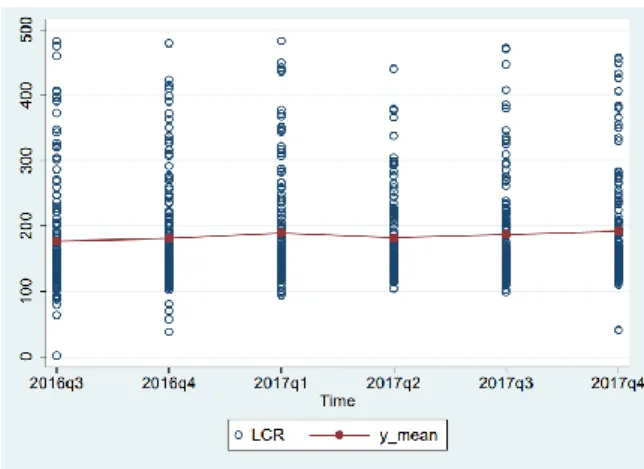
seem that LCR affects negatively the loans provided by banks, despite the high variance of the results. However, when the data is aggregated at bank level (figure 4), it seems that the correlation between the LCR and the ratio of total loans to total assets held is positive,
showing a different relationship compared to when the data is aggregated at the country level. This can be explained by the fact that the correlation does not control for other variables. When looking at figure 5, it is possible to visualize that the loans of the banks weighted on their total assets has a great level of variance. The average is around 50%, which clearly indicates the importance of the loans provided by banks in their activity. On the other hand, in figure 6 it is possible to conclude that there is also a significant variance of the LCR among the sample chosen. While most of banks comply with an LCR of 100%, the average in the sample is very close to 200%, which proves that most of the banks set their LCR significantly higher than the minimum requirement. Furthermore, in figure 7, it is possible to visualize a slightly positive relationship between the regulatory requirements of the CET1 ratio and LCR.
Regressions computed and conclusions
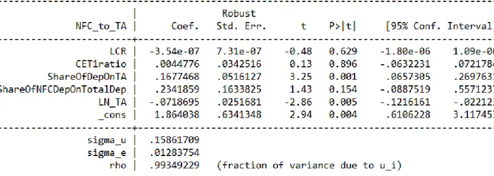
In the first place, it was studied the impact of the LCR on banks’ lending26. We found evidence that the LCR does not have any impact on the loans provided by banks, either at an aggregated level, or separately to either households or non-financial corporations. This conclusion was taken when looking at the P-value for the specific regressions presented in tables 3 4 and 5, which are 0.945, 0.231 and 0.629 respectively. This can be explained by the fact that a higher LCR ratio will also mean that the banks may be viewed as more financial stable, and this can enable the bank to provide for a higher amount of loans (BIS, 2016)
26 Please see tables 3,4 and 5 for reference
16
Secondly, we have performed a more detailed analysis on the LCR ratio by using the ratio of high-quality liquid assets to total assets. That is, taking into account only a part of the LCR (the numerator, excluding therefore the net stressed outflows which are based on
additional assumptions27 in order to be computed, which may distort the analysis).
Under my estimation in tables 6 and 7, I found that the lowest BIC criterion28 for the impact of the HQLAs on total loans and on loans to non-financial corporations respectively was found for the third column29. On the other hand, the lowest BIC criterion for the impact of the HQLAs on loans to households was found for the second column30 in table 8. These
regressions included the following regressors: HQLA, CET1 ratio, the shortfall to an LCR of 100%, the share of deposits on total assets, the overnight deposits weight on total deposits, the share of household’s deposits or non-financial corporation deposits to total deposits, and the logarithm of banks’ total assets.
The HQLAs ratio to total assets, the share of deposits on total assets, and the logarithm of total assets were significant mostly at the 1% P-value level. The coefficient on the HQLA ratio to total assets is significant and negative for all of the 3 regressions previously pointed out in tables 6,7 and 8, columns 3, 3 and 2 respectively. The coefficients on the HQLAs are -0.305, -0.127 and -0.173 for the regressions on which the dependent variable is total loans, loans to households, and loans to non-financial corporations respectively, which are divided
27 The net stressed outflows depend on cash outflows and cash inflows. The cash outflows depend on, for
example, retail deposits or secured funding, while cash inflows depend on, for example, secured lending. The cash outflows and inflows are subjected to calibrated run-off rates based on information from the financial crisis, internal stress scenarios of banks, and existing regulatory and supervisory standards. For more detail, please see: https://www.bis.org/publ/qtrpdf/r_qt1212g.pdf
28 The Bayesian information criterion (BIC) can be used as a criterion to compare different models. The criterion
is based on the likelihood function as well as the number of regressors to be estimated. In order to better fit a specific model, we may add regressors as it may increase the likelihood by adding parameters. However, this may also cause a problem of overfitting in which the model can include variables of no interest which may deteriorate the model’s explanatory power. The BIC criterion takes this into account since it has a penalty term for the number of parameters which are included into the model.
29 The lowest BIC criterion in table 6 and 7 is -3961.828 and -4615.051 respectively, in the third column 30 The lowest BIC criterion in table 8 was -4450.203 in the second column
17
by banks’ total assets. This means that on average, if the ratio of HQLAs to total assets increases by 1%, the ratio of total loans to total assets provided by a specific bank is expected to decrease by 0.305% (0.173% in case of loans provided only to households, and 0.127% in case of loans provided only to non-financial corporations) in that period.
However, the CET1 ratio and the shortfall to a 100% LCR ratio was rarely significant for all of the regressions computed, which may indicate that the HQLA could absorb the positive effects of a financial stable institution. The share of overnight deposits to total
deposits on table 6 was significant in most of the regressions computed. Although the share of deposits of non-financial corporations to total deposits was not a significant variable in table 7, the share of household’s deposits to total deposits was a very significant variable on table 8. This may indicate that the deposits from households held by a bank is an important variable to predict the loans provided to households, while in the case of loans provided to non-financial corporations, it is more important the shares of deposits to total assets held by the bank. Furthermore, the Macroeconomic variables (EOINA rate, GDP growth rate, unemployment rate, house prices growth and the difference between lending margins) were not significant in any of the computed regressions. This may indicate that the loans provided by each bank do not depend directly on the economic performance of the country in which the bank is headquartered. This could be explained by the fact that the regression with the
macroeconomic variables such as the GDP growth, unemployment rate, and house prices growth, do not take into account the different dimensions of banks situated in each country, in order to give more weight to countries which have headquartered in them banks that provide a greater amount of loans31. Moreover, it shall also be taken into account that there is a free market installed in Europe, and there is a great interconnectedness between the countries
31 This may indicate that the use of a cross term between macroeconomic variables and banks’ dimension
18
performance, which may indicate that it is not important to separate the different growths per country, as banks headquartered in a specific country also provide loans to other countries within Europe, and may also have subsidiaries headquartered in a different country, which may further increase the level of interconnectedness between loans provided by banks headquartered in different countries.
Conclusion
While there has been a lot of studies provided for both positive and negative effects of capital regulation, fewer studies have been provided regarding liquidity regulation. One of the main reasons is that minimum liquidity requirements are relatively new, while minimum capital requirements have been implemented since Basel I. In this paper, I focused on the impact of liquidity regulation on banks’ credit supply. I found that there is evidence that liquidity requirements affect negatively banks’ ability to provide loans. Households are more affected by liquidity restrictions than financial corporations. This results were found in a non-stressed period for the high-quality liquid assets ratio to total assets. On the other hand, I was not able to find a significant impact of the LCR on the loans provided by banks, which is a result that supports the use of the LCR as a minimum regulatory requirement. However, the high-quality liquid assets represent the most important component of the LCR, as it can also be viewed as a measure of liquidity that banks held, and this measure can have an impact on the credit supply. The different results on the impacts may be explained by the fact that the LCR is a ratio which takes into account additional assumptions on a banks’ liquidity position. Moreover, since the ratio is publicly disclosed, the higher the ratio is, the more the bank is seen as being financial stable by investors, which can further improve banks’ credit supply.
19
Annex 1
Equation 1: LCR ratio calculation𝐿𝑖𝑞𝑢𝑖𝑑𝑖𝑡𝑦 𝐵𝑢𝑓𝑓𝑒𝑟
𝑁𝑒𝑡 𝐿𝑖𝑞𝑢𝑖𝑑𝑖𝑡𝑦 𝑂𝑢𝑡𝑓𝑙𝑜𝑤𝑠 𝑜𝑎𝑣𝑒𝑟 𝑎 30 𝑐𝑎𝑙𝑒𝑛𝑑𝑎𝑟 𝑑𝑎𝑦 𝑠𝑡𝑟𝑒𝑠𝑠 𝑝𝑒𝑟𝑖𝑜𝑑= 𝐿𝑖𝑞𝑢𝑖𝑑𝑖𝑡𝑦 𝐶𝑜𝑣𝑒𝑟𝑎𝑔𝑒 𝑅𝑎𝑡𝑖𝑜 (%)
Table 1: LCR Minimum requirements for32
Equation 2: ILG ratio visualization for a specific credit institution 𝐻𝑖𝑔ℎ 𝑞𝑢𝑎𝑙𝑖𝑡𝑦 𝑙𝑖𝑞𝑢𝑖𝑑 𝑎𝑠𝑠𝑒𝑡𝑠
𝑁𝑒𝑡 𝑠𝑡𝑟𝑒𝑠𝑠𝑒𝑑 𝑜𝑢𝑡𝑓𝑙𝑜𝑤𝑠 > x%
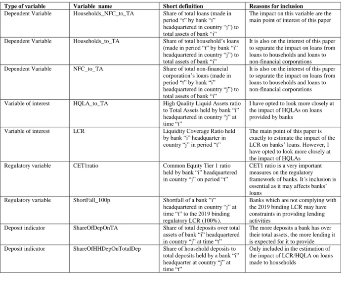
Table 2: Definitions and explanations of variables included in regressions
Type of variable Variable name Short definition Reasons for inclusion
Dependent Variable Households_NFC_to_TA Share of total loans (made in period “t” by bank “i” headquartered in country “j”) to total assets of bank “i”
The impact on this variable are the main point of interest of this paper Dependent Variable Households_to_TA Share of total household’s loans
(made in period “t” by bank “i” headquartered in country “j”) to total assets of bank “i”
It is also on the interest of this paper to separate the impact on loans from loans to households and loans to non-financial corporations Dependent Variable NFC_to_TA Share of total non-financial
corporation’s loans (made in period “t” by bank “i” headquartered in country “j”) to total assets of bank “i”
It is also on the interest of this paper to separate the impact on loans from loans to households and loans to non-financial corporations Variable of interest HQLA_to_TA High Quality Liquid Assets ratio
to Total Assets held by bank “i” headquartered in country “j” at time “t”
I have opted to look more closely at the impact of HQLAs on loans provided by banks
Variable of interest LCR Liquidity Coverage Ratio held by bank “i” headquarter in country “j” in period “t”
The main point of this paper is exactly to estimate the impact of the LCR on banks’ loans. However, I have opted to look more closely at the impact of HQLAs
Regulatory variable CET1ratio Common Equity Tier 1 ratio held by bank “i” headquartered in country “j” on period “t”
CET1 ratio is a very important measures on the regulatory framework of banks. It´s inclusion is essential as it may affects banks’ loans
Regulatory variable ShortFall_100p Shortfall of a bank ”i” headquartered in country “j” at time “t” to the 2019 binding regulatory LCR (100%).
Banks which are not complying with the 2019 binding LCR may have constraints in providing lending activities
Deposit indicator ShareOfDepOnTA Share of total deposits over total assets of bank “i” headquartered in country “j” at time “t”
The more deposits a bank has over their total assets, the more lending it is expected for it to provide Deposit indicator ShareOfHHDepOnTotalDep Share of household deposits to
total deposits held by a bank “i” headquarter at country “j” at time “t”
Only included in the estimation of the impact of LCR/HQLA on loans made to households
32 Retrieved from: https://www.bis.org/bcbs/basel3/basel3_phase_in_arrangements.pdf
1 January 2015 1 January 2016 1 January 2017 1 January 2018 1 January 2019
20
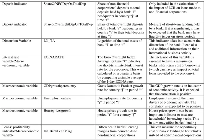
Deposit indicator ShareOfNFCDepOnTotalDep Share of non-financial corporations’ deposits to total deposits held by a bank “i” headquarter in country “j” at time “t”
Only included in the estimation of the impact of LCR on loans made to non-financial corporations Deposit indicator ShareofOvernightDepOnTotalDep Share of total overnight deposits
held by bank “i” headquarter in country “j” to their total deposits at time “t”
Measure of short-term funding held by a bank. If it is significant, it may be expected that the bank may have liquidity issues on stress periods Dimension Variable LN_TA Logarithm of the total assets of
bank “i” at time “t” This indicator takes into account the dimension of the bank. It can also add additional information on their international business activity Interest rate
variable/Macro -economic variable
EOINARATE The Euro Overnight Index Average for time “t” indicates the short-term interbank interest rate for the euro-zone. This was calculated on a quarterly basis by computing a simple average of the 1-day EOINA rate.
The inclusion of this variable is essential to have a measure on banks’ short-term cost of borrowing (which can have an impact on total loans provided to the economy). Macroeconomic variable GDPgrowthpercountry Gross Domestic Product growth
rate for country “j” in period “t”
The GDP growth rate is an indicator of economic activity. It is expected that the correlation is positive Macroeconomic variable Unemploymentrate Unemployment rate for country
“j” in period “t”
Employment is one of the main drivers of economic activity. The correlation is expected to be positive Macroeconomic variable Housepricesgrowth House prices growth rate in
period “t” for a country “j” House prices growth can be an important indicator to measure households’ borrowing needs. This in turn may affect banks’ lending Loans’ profitability
indicator/Macroeconomic variable
DiffBankLendMarg
Difference in banks’ lending margins from households to non-financial corporations
This can measure the opportunity cost of banks’ lending to households instead of non-financial corporations
Figure 1: XTOVERID results in Stata for a test of Fixed vs Random effects
21
Figure 3: Linear correlation between total loans Figure 4: Linear Correlation between total loans and the Liquidity Coverage Ratio and the Liquidity Coverage Ratio aggregated per country
Figure 5: Loans’ weight on total assets per bank: Figure 6: Liquidity Coverage Ratio: average average and individual observations across time and individual observations across time
Figure 7: Linear prediction between the CET1 ratio and the LCR
22 Table 3: Impact of the LCR on total bank loans
Table 4: Impact of the LCR on total bank loans to households
23
Table 6: Impact of HQLA ratio to total assets on total bank loans
24
25
26
Annex 2
The Basel III framework was introduced in 2010 in order to revise areas such as market risk, counterparty credit risk and securitization in order to better capture the associated risks (Ingves, 2018).
Although the leverage ratio was implemented by the Basel III framework in order to bring a risk-insensitive measure (BIS 2016), there was also still a need for more risk-sensitive indicators, as there were some risks that the Basel II framework did not addressed. A greater interconnectedness between international financial institutions was proven to exist, which consequently created a global systemic risk that had to be taken into account in the new Basel framework (BIS, 2010). Therefore, a macroprudential perspective was implemented to the regulatory framework (Ingves, 2018). The Basel committee not only developed a
countercyclical capital buffer to build banks’ prudential capital in periods of excessive growth, but also built buffers to address the interconnectedness of the European financial system. Global systemically important banks (G-SIBs), domestic systemically important banks (D-SIBs) and other systemically important institutions (O-SIIs) could be assigned additional buffers for their systemic importance in an international or domestic level. Also, capital conservation buffers were implemented in the Basel III framework, which created an incentive for banks to limit discretionary distributions in times of stress (BIS 2010). Pillar 2 (banking supervision) and Pillar 3 (transparency and market discipline) were reinforced in Europe with the implementation of the Capital Requirements Regulation (CRR)33, Capital
33 For reference, please see the Official Journal of the European Union:
27
Requirements Directive (CRD)34, and Bank Recovery and Resolution Directive (BRRD)35. The competent authorities, mainly the ECB and the European Banking Authority, were better equipped with tools to impose restrictions on European banks in order to mitigate the
likelihood and the impact of banks’ failure. Moreover, when not possible to prevent the failures, what is relevant is to avoid the burden to fall on European taxpayers. In the United States, the Financial Stability Board (FSB) implemented the Total Loss-Absorbing Capacity (TLAC) standard, for specific global systemically important banks (G-SIBs) which would prevent an unorderly failure of the banks in which public funds could need to be used.
34 For reference, please see the Official Journal of the European Union:
https://eur-lex.europa.eu/legal-content/EN/TXT/PDF/?uri=CELEX:32013L0036&from=EN
35 For reference, please see the Official Journal of the European Union:
28
Annex 3
Since the benefits of a sound banking system are very hard to measure, not many studies have quantified them. One of the main benefits of liquidity regulation is that it “may reduce the contraction of bank credit in response to liquidity shocks, thereby resulting in a lower
reduction in aggregate output associated with banking crises than in its absence” (BIS, 2016). In fact, in a study on liquidity risk management and credit supply by US banks in the 2008-2009 financial crisis, by analyzing how banks adjusted their holding of cash and other liquid assets, it was found that “banks with more illiquid asset portfolios, … , increased their
holdings of liquid assets and decreased lending. Most of the decline in bank credit production during the height of the crisis can be explained by liquidity risk exposure.” (Cornett, McNutt, Strahan and Tehranian, 2011). Similar results were also found in a study in which the authors used bank-firm level data, in order to study the causal relation between French banks’
liquidity risk and their lending capacity in the period of 2007-2008. The study supports the rationale of the liquidity regulation. The authors showed that “Lower funding risk and a lower maturity mismatch immunise banks from funding shocks. This in turn allows banks to
continue extending longterm loans to firms in times of funding stress. Such a regulation might thus support economic growth during periods of downturn by ensuring that banks continue their role of long-term funding providers for firms that cannot access alternative financing sources.” (Pessarossi and Vinas, 2015).
In fact, the argument of a positive impact of liquidity regulations on the lending capacity of banks would be counter-intuitive in a non-stress scenario. However, in a stress scenario, liquidity regulations may indeed help to provide for liquidity buffers which may attenuate the negative impact on the lending provided by credit institutions.
29
It should also be referred that a net benefit analyzes on the costs and benefits of the regulation is very difficult to perform. The reason is that it is very hard to quantify the benefits of liquidity regulation in terms of the events it avoids, since the regulation prevents this empirical events to occur in the first place. Furthermore, the benefits arising from the lower costs and likelihood of bank failure are very hard to quantify. In fact, “a comprehensive empirical assessment of the net welfare benefits of liquidity regulations has not been
30 References
European Central Bank. 2009. “The financial crisis and the role of central banks: The experience of the ECB.”. Keynote address by Jean-Claude Trichet, President of the ECB. https://www.ecb.europa.eu/press/key/date/2009/html/sp090529.en.html
N Banerjee, Ryan. and Mio, Hitoshi. 2015. “The impact of liquidity regulation on banks”. Bank of England Staff Working Paper No. 536: 1-44
Bank for International Settlements. 2013. “Basel III phase-in arrangements”. https://www.bis.org/bcbs/basel3/basel3_phase_in_arrangements.html
Bank for International Settlements. 2010. “Basel III: a global regulatory framework for more resilient banks and banking systems”. https://www.bis.org/publ/bcbs189_dec2010.htm Bank for International Settlements. 2013. “Basel III: The Liquidity Coverage Ratio and liquidity risk monitoring tools”. https://www.bis.org/publ/bcbs238.htm
Bank for International Settlements. 2016. “Literature review on integration of regulatory capital and liquidity instruments”. https://www.bis.org/bcbs/publ/wp30.htm
Cornett, Marcia Millon., McNutt, Jamie John., E.Strahan, Philip., and Tehranian, Hassan. 2011. “Liquidity risk management and credit supply in the financial crisis”. Journal of Financial Economics, 101(2): 297-312
Pessarossi, Pierre. and Vinas, Frédéric. 2015. “The supply of long-term credit after a funding shock: evidence from 2007-2009”. Document de travail du Centre d’Economie de la
Sorbonne 2015.73 – ISSN : 1955-611X.
Bonner, Clemens. and Eijffinger, Sylvester. 2012. “The Impact of the LCR on the Interbank Money Market”. De Nederlandsche Bank Working Paper No.364: 1-24
Wooldrige, Jeffrey Marc. 2001. Econometric Analysis of Cross Section and Panel Data. The MIT Press
Wooldrige, Jeffrey Marc. 2013. Introductory Econometric: A Modern Approach 5th edition. Huang, Rocco. and Ratnovski, Lev. “The dark side of bank wholesale funding”. European Central Bank Working Paper No.1223: 1-41
DeYoung, Robert. and Jang, Karen. “Do banks actively manage their liquidity?”. Journal of Banking & Finance, 66: 143-161
De Bandt, Olivier. and Chahad, Mohammed. 2015. “A DGSE model to assess the post crisis regulation of universal banks” , Mimeo, University of Paris Ouest and Banque de France-Autorité de Contrôle Prudentiel et de Résolution
31
Covas, Francisco. and C.Driscoll, John. 2014. “Bank Liquidity and Capital Regulation in General Equilibrium”. Finance and Economics Discussion Series, Federal Reserve Board. De Nicolò G, A Gamba and M Lucchetta. 2014. “Microprudential regulation in a dynamic model of banking”. Review of Financial Studies, 27(7): 2097-2138
Basel Committee on Banking Supervision. 2018. “Basel III: Are we done now?” Keynote speech by Stefan Ingves, Chairman of the Basel Committee on Banking Supervision. https://www.bis.org/speeches/sp180129.htm
Bonfim, Diana. and Kim, Moshe. 2013. “Liquidity risk in banking. Is there herding?”. https://www.bportugal.pt/sites/default/files/2013cfi_paper6_e.pdf
Strahan, Philip. 2012. “Liquidity Risk and Credit in the Financial Crisis”. FRBSF Economic Letter.
https://www.frbsf.org/economic-research/publications/economic-letter/2012/may/liquidity-risk-credit-financial-crisis/
European Central Bank. 2017. “Assessment of ‘Failing or Likely to fail’ for Veneto Banca Società per Azioni”.
https://www.bankingsupervision.europa.eu/ecb/pub/pdf/ssm.2017_FOLTF_ITVEN.en.pdf European Central Bank. 2017. “Assessment of ‘Failing or Likely to fail’ for Banco Popular Espanõl”
https://www.bankingsupervision.europa.eu/ecb/pub/pdf/ssm.2017_FOLTF_ESPOP.en.pdf Bech, Linnemann. And Keister, Todd. 2012. “On the liquidity coverage ratio and monetary policy implementation”.https://www.bis.org/publ/qtrpdf/r_qt1212g.pdf