Proceedings of 2008 ASME Summer Heat Transfer Conference HT2008 August 10-14, 2008, Jacksonville, Florida, USA
HT2008-56421
THREE-DIMENSIONAL CFD MODELLING AND ANALYSIS OF THE THERMAL
ENTRAINMENT IN OPEN REFRIGERATED DISPLAY CABINETS
Pedro Dinis GasparUniversity of Beira Interior
Electromechanical Engineering Department Covilhã, Portugal
L.C. Carrilho Gonçalves University of Beira Interior
Electromechanical Engineering Department Covilhã, Portugal
R.A. Pitarma
Polytechnic Institute of Guarda - School of Technology and Management Mechanical Engineering Department
Guarda, Portugal
ABSTRACT
This study presents a three-dimensional Computational Fluid Dynamics (CFD) simulation of the air flow pattern and the temperature distribution in a refrigerated display cabinet. The thermal entrainment is evaluated by the variations of the mass flow rate and thermal power along and across the air curtain considering the numerical predictions of abovementioned properties. The evaluation on the ambient air velocity for the three-dimensional (3D) effects in the pattern of this type of turbulent air flow is obtained. Additionally, it is verified that the longitudinal air flow oscillations and the length extremity effects have a considerable influence in the overall thermal performance of the equipment. The non uniform distribution of the air temperature and velocity throughout the re-circulated air curtain determine the temperature differences in the linear display space and inside the food products, affecting the refrigeration power of display cabinets.
The numerical predictions have been validated by comparison with experimental tests performed in accordance with the climatic class n.º 3 of EN 441 Standard (Tamb = 25 ºC,
φamb = 60%; vamb = 0,2 m s-1). These tests were conducted using
the point measuring technique for the air temperature, air relative humidity and air velocity throughout the air curtain, the display area of conservation of food products and nearby the inlets/outlets of the air mass flow.
INTRODUCTION
The open refrigerated display cabinets suffer alterations of their thermal performance due to variations of the ambient air conditions (air temperature, relative humidity and magnitude
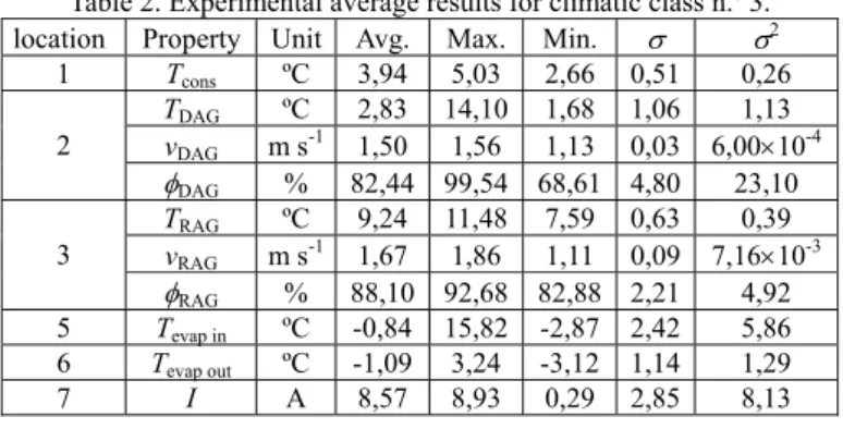
and orientation of the air velocity). The location of the air conditioning system discharge grilles, the mass flows originated by pressure differences due to the openings to the exterior, and the air flow perturbation due to the circulation of consumers nearby the frontal opening of the display cabinet, among others, affects the re-circulated air curtain behavior and consequently the global thermal performance of the equipment. The ambient air infiltration load is around 72 % of the cooling load of open refrigerated display cabinets [1]. The effectiveness of the air curtain as aerothermodynamics barrier varies due thermal and mass diffusive effects that affect the thermal entrainment, flow instabilities and boundary effects, among others leading to a minor conservation quality of the food products and greater energy consumption and costs. It is important to state that the energy spent with the commercialization of food products stored in cold is about 50 % of the total consumption of energy of a typical supermarket [2], being particularly affected by the open display cabinets electrical energy consumption. The growing of energy consumption in the commercial sector is due to the increasing demand of large quantities of perishable food products in urban areas, and a more effective rigorous regulation of the sector as well as by the exigencies of the consumers concerning quality and food safety. In Figure 1.a) is exposed a typical configuration of an open vertical refrigerated display cabinet. The air is sucked at the return air grille (RAG) through the fans located in front of the evaporator. During the passage through the evaporator, the air is cooled below the conservation temperature of the perishable products exposed in the shelves. This air mass flow rate is conducted to a rear duct, where part
of this air mass is discharged at low velocity across the back internal panel perforation inside conservation space. Most part of this air mass flow will supply the re-circulated air curtain, which will develop vertically between the discharge air grille (DAG) and the RAG. The air curtain attempts to reduce the external infiltration of air from outside at higher dry temperature and specific humidity. The empirical design of the re-circulated air curtain result in a higher thermal entrainment of ambient air by the length extremities of the equipment as described by Gray et al. [3] and D’Agaro et al. [4]. Also, a leakage of refrigerated air from the bottom part of the vertical opening to the surroundings (cold leg effect) occurs, losing energy to outside. Those factors, allied to the remaining heat gain components [2], leads to an increasing of the thermal load and consequently higher energy consumption. ASHRAE [5] expresses that the reduction of the thermal load is the first step for a better energy efficiency of the refrigeration equipments through the optimization of the air curtain, allowing a reduction in the thermal entrainment with ambient air and a better aerothermodynamics behavior of the air curtain, being the returned air to the evaporator at a lower temperature. Due to its influence, most of the present research in this field is devoted to the air curtain devices installed in open refrigerated display cabinets. The study provided by Navaz et al. [6] presents the state of the art of the numerical and experimental investigations concerning the air curtains thermal performance and indicates that there is still a need in identifying, quantifying and optimizing all the variables involved in the overall aerothermodynamics performance of re-circulated air curtains. The research works on air curtains are mainly related with heat and mass transfer’s studies and the evaluation of the heat transfer in air curtains with: an impingent jet of several angles, some initial velocities and temperatures and different thicknesses and with generation/suppression of turbulence inside the air stream [7-12]. The main outcomes of these studies are the determination of air curtain thermal efficiency and the overall energetic performance of the aerothermodynamics system. Other works have evaluated the performance of air curtains subjected to external perturbations and investigate the thermal interaction between air curtains and the controlled air space. Several studies combined analytical and experimental procedures conducted according to EN 441 Standard [13] using several experimental measurement techniques like thermocouple thermometry, hot wire/film anemometry, laser Doppler anemometry, digital particle image velocimetry, hygrometry, tracer gases, infrared thermography, among others. Gaspar et al. [1, 14-15] developed experimental studies to evaluate the impact on the thermal performance of a refrigerated display cabinet under different ambient air conditions. They also investigate the three dimensional (3D) pattern of the thermal entrainment in re-circulated air curtains and its effects on the thermal performance, like the distribution of the air temperature and humidity in a refrigerated display cabinet. Considering the increasing broaden use of CFD as an expedite and rational analysis method, the study provided by
Smale et al. [16] and Norton & Sun [17] presented a review of the application of CFD and other numerical modeling techniques to the prediction of air flow in refrigerated food applications including cool stores, transport equipments and retail display cabinets. CFD studies combined with experimental techniques have been developed to evaluate both air curtain aerothermodynamics performance and energy efficiency of vertical open refrigerated display cabinets. The two- (2D) and three-dimensional (3D) CFD models developed by Cortella et al. [18], Ge & Tassou [19], Navaz et al. [20], Axell & Fahlén [21], Navaz et al. [22], Foster et al. [23], Chen & Yuan [24], and D’Agaro et al. [4] were devoted to: study the flow field characteristics and air curtain efficiency through the quantification of the entrained air into the cabinet; evaluate the thermal characteristics considering different test specification; investigate the influence of the air curtain height, width and inlet velocity on the efficiency; address those parameters that have significant effects on the amount of entrained air in an open refrigerated display cabinet; study the effects of ambient air temperature, indoor relative humidity, ambient air flow, air supply velocity, air flow from perforated back panels and night covers on the performance of a refrigerated display cabinet; and analyze the effects of the cabinet length, of the warm air curtain and of longitudinal ambient air movement on the temperature field distribution. But none of these studies have modeled the several devices that make part of the refrigeration system. The work described in this paper intends to combine the characteristics of the aforementioned works, thus performing a 3D CFD simulation of an open vertical display cabinet that considers the ambient air flow parallel to the display cabinet frontal opening in order to evaluate the thermal entrainment across the air curtain and along the cabinet’s length and the aerothermodynamics performance of the air curtain. EXPERIMENTAL TESTING
The experimental study follows the methodology provided by [13] for the test of open refrigerated display cabinets concerning the M-package temperature class M1 (-1 ºC < Tcons
< 5 ºC) and for the test room climatic class n.º 3 (Tamb = 25 ºC,
φamb = 60 %, vamb = 0,2 m s-1, being the air movement
longitudinal to the length of the equipment). The dimensions of the display cabinet in the present work are 1900 × 796 × 1911 mm (L × W × H). It has four shelves and a well tray. The refrigeration system uses in-situ a condenser-compressor unit. The experimental tests were performed inside a climatic chamber Aralab - Fitoclima 650000 EDTU. Figure 1.b) and c) presents the cabinet location and orientation inside the climatic chamber, the distribution of the test probes as well as the probes positioning system. It was used a data acquisition system Intab PC-Logger 3100 to connect the probes exposed in Table 1, distributed inside the refrigeration equipment as presented in Figure 2. Also in Figure 2 are presented the location and dimensions of the: width of the air curtain (bsupply
= 60 mm); height of the opening (Hc = 1209 mm); and the
a) Cabinet typical configuration. b) Cabinet location and probes distribution. c) Probes (T, v, ω) positioning system. Figure 1. Cabinet location inside climatic chamber and test probes distribution.
Table 1. Description of the test probes and its location.
n. Location Type Property Ref.
1 conservation K-type thermocouple Temperature Tcons
K-type thermocouple Temperature TDAG
Hot-wire anemometer Velocity vDAG
2 DAG
Hygrometer Rel. humidity φDAG
K-type thermocouple Temperature TRAG
Hot-wire anemometer Velocity vRAG
3 RAG
Hygrometer Rel. humidity φRAG
4 M-package K-type thermocouple (contact) Temperature (Products) Tprod
5 Evaporator (upstream) K-type thermocouple (contact) Temperature (Surface) Tevap_in
6 Evaporator (downstream) K-type thermocouple Temperature Tevap_out
7 Power source Ammeter (clamp-on) Electric current I
In order to consolidate the measurements, a thermo-anemometer AM 4003 was used to measure the air temperature and velocity near the DAG and RAG, the refrigeration unit and perforated back panel.
In the same locations, the pressure loss was measured using a micro-manometer Air Instruments Resources MP3KDS. The internal surface temperatures were obtained with K-type thermocouple contact probe using a digital thermometer FLUKE 51. The main procedure followed to accomplish the experimental tests begin with the start up and running of the climatic chamber’s air conditioning system during 3 hours before starting up the refrigeration system of the display case, in order to reach indoor air temperature and relative humidity steady states. Then, it was considered a delay of another 2 hours to accomplish the desired conservation air temperature inside the refrigerated display case (total time: 8 hours), before loading it with the M-packages at the adequate conservation temperature. The experimental data was collected during 24 hours when the steady state test conditions were reached. It had been done several series of experimental tests to evaluate the influence of the surrounding air in the air temperature, velocity and humidity inside conservation space. The average measured values (last 12 hours) of the physical properties were calculated in order to reduce the experimental results uncertainty, concerning the repeatability of the measurements.
a) Probes location. b) width-height (y-z plane). c) length-height (x-z plane)
A probes positioning system was used to evaluate the 3D effects of the thermal entrainment in the air curtain (see Figure 2.c). This system was settled in each shelf of the equipment, and it measures the air temperature, relative humidity and velocity for 3 positions across the air curtain (y/b = 0; 0,5; 1 – see Figure 2.b) and for 8 vertical cross-sections along the equipment length (x/L – see Figure 2.c). Since the equipment has 1800 mm long, the positioning system measures the properties values in 240 mm increments. The positioning system takes one minute to move between positions to reduce the flow perturbation. Also, the data measurements of the values of the properties were done after one minute staying in the defined position to ensure the flow stabilization. Figure 2 presents the grid measuring points represented by red dots (z).
In Table 2 are presented the average temporal and spatial values of the parameters since they had been obtained in transient state and for different spatial locations along length (probes location n.º 1). It is also presented the statistical parameters of the properties variation: maximum and minimum values; standard deviation (σ) and the variance (σ2).
Table 2. Experimental average results for climatic class n.º 3.
location Property Unit Avg. Max. Min. σ σ2
1 Tcons ºC 3,94 5,03 2,66 0,51 0,26 TDAG ºC 2,83 14,10 1,68 1,06 1,13 vDAG m s-1 1,50 1,56 1,13 0,03 6,00×10⁻⁴ 2 φDAG % 82,44 99,54 68,61 4,80 23,10 TRAG ºC 9,24 11,48 7,59 0,63 0,39 vRAG m s-1 1,67 1,86 1,11 0,09 7,16×10⁻³ 3 φRAG % 88,10 92,68 82,88 2,21 4,92 5 Tevap in ºC -0,84 15,82 -2,87 2,42 5,86 6 Tevap out ºC -1,09 3,24 -3,12 1,14 1,29 7 I A 8,57 8,93 0,29 2,85 8,13 CFD MODELLING
The turbulent air flow and non-isothermal heat transfer process presented in this simulation consists in a 3D and steady state mathematical model. The basic equations governing the transport phenomena in the inwards of the refrigerated display cabinet are continuity, momentum and energy [25].
Mathematical formulation
These governing equations for the averaged flow of an incompressible fluid can be written in the general form by Equation 1 for a dependent variable φ (=1 for the continuity equation, = vi , = T, for momentum and energy equations
respectively). Γφ is the diffusion coefficient and Sφ represents
the source term.
φ φ φ φ ρ S x v xk k ⎟⎟⎠= ⎞ ⎜⎜ ⎝ ⎛ ∂ ∂ Γ − ∂ ∂ (1)
The air is considered as an ideal gas, whose state equation relates the parameters of the substance at equilibrium gas phase
state accurately. The buoyancy-driven forces are treated as a source term in the momentum equations.
The energy equation is developed as a function of temperature in a steady state regime with constant specific heat. Further simplifications are accomplished despising viscous dissipation due to the flow characteristics.
The turbulence was modeled with two equation (one for turbulent kinetic energy and another for dissipation rate of turbulent energy) RNG k-ε model [26]. The set of model equations presented above (Equation 1) is suitable for fully turbulent flow. Near the walls, the viscous effects prevail over the turbulent ones. To account for viscous effects and high gradients in the proximities of the walls, the turbulence model equations are used in conjunction with the empirical wall functions. The complete description and implementation details of the wall functions in turbulence models can be found in Rodi [27] and Launder et al. [28].
The heat gain of the display cabinet through radiation is considered using a surface to surface radiation model based in the surfaces view factors calculation, since it is one of the most significant components of the cooling load for this type of display cabinets [1].
Geometry and computational mesh
The 3D geometry for the CFD model closely followed the real one. It was used an automatic orthogonal unstructured mesh generator (Gambit) included in the code. The control volume discretization of the refrigerated cabinet and the external surroundings require a computational grid with 5684513 control volumes. The model requires such high number of control volumes due to the geometrical distances variations near the end walls of the equipment. This mesh refinement allows the development of a high quality grid without high skewness levels and aspect ratios.
Numerical model
The mathematical model is a set of coupled non-linear partial differential equations, expressing mass, momentum and energy conservation which should be simultaneously and interactively solved. The present study makes use of a commercial CFD code Fluent 6.3.26 for the solution of this set of equations. The computational procedure used was based on a numerical iterative process using the PISO (Pressure-Implicit with Splitting of Operators) algorithm [29] for the pressure-velocity coupling. This algorithm was derived from the SIMPLE (Semi-Implicit Method for Pressure-Linked Equations) algorithm [30], but as presented by Jang et al. [31] it has higher performance and it is more efficient. The equations were discretized in the control volume form using the MUSCL (Monotone Upstream-Centered Schemes for Conservation Laws) differencing scheme. The MUSCL scheme proposed by Van Leer [32] relies on the Central Differencing Scheme (CDS) and on the Second Order Upwind (SOU) differencing scheme) [30]. It is a differencing scheme with higher spatial precision for all types of computational grids and
for complex flows, since it reduces the numerical diffusion. Due to convergence difficulties, the Upwind differencing scheme (UDS) was used to discretize the turbulent quantities.
The hardware used to run the models was a server with an Intel Xeon DualCore running at 2,33 GHz (4 MBytes internal cache) with 12 GBytes RAM.
Boundary conditions
In the computational domain are imposed the boundary conditions (BC) of common practice in numerical simulations.
- Inlet boundary conditions
At the mass flow rate inlets such as DAG, the perforation of the internal back panel and the room inlet wall are specified the experimental average values. The turbulence parameters are specified in terms of hydraulic diameter and turbulence intensity like exposed in Equation 2. Table 3 present the values specified at the different inlet boundary conditions.
( )
Re 18 16 , 0 − = Dh t I (2)The mass flow rate through the perforated internal back panel (PIBP) is determined by mass conservation:
DAG RAG PIBP out
in m m m m
m& = & ⇔ & = & − & (3)
Table 3. Inlets boundary conditions.
Zone Parameters Variable Unit Value
Velocity vDAG m s-1 1,50 Temperature TDAG ºC 2,83 Hydraulic diameter Dh m 0,12 Turbulence intensity It % 4,90 DAG Emissivity εDAG – 0,90
Mass flow rate m&PIBP kg s-1 0,13
Temperature TPIBP ºC 1,00 Hydraulic diameter Dh mm 4,25 Turbulence intensity It % 7,19 PIBP Emissivity εPIBP – 0,90 Velocity vroom,in m s-1 0,20 Temperature Troom,in ºC 25,00 Hydraulic diameter Dh m 2,35 Turbulence intensity It % 4,41 Emissivity εroom,in – 1,00 Room inlet
Black body temperature Tbb ºC 8,17
- Outlet boundary conditions
The outlet BC are specified at the RAG and the room outlet wall. The values specified are based on the experimental average values. The turbulence parameters are specified by the formulation presented for inlet BC. Table 4 presents the values specified at the different outlet boundary conditions.
Table 4. Outlet boundary conditions.
Zone Parameters Variable Unit Value
Velocity vRAG m s-1 -1,67 Temperature TRAG ºC 9,24 Hydraulic diameter Dh m 0,17 Turbulence intensity It % 4,63 RAG Emissivity εRAG – 0,90 Velocity vroom,out m s-1 -0,2 Temperature Troom,out ºC 25,00 Hydraulic diameter Dh m 2,35 Turbulence intensity It % 4,41 Room outlet Emissivity εroom,out – 0,90
- Heat flux boundary conditions
For the walls not considered in the heat transfer calculus an adiabatic BC is defined. However, the heat flux BC is used to simulate the heat generated by the illumination (85% for fluorescent lamp) and the heat flux through conduction across the material layers that compose the walls of the equipment. The heat fluxes across the walls of the equipment are specified as BC (see Table 5), using the Fourier Law with a global heat transfer coefficient determined by conductive thermal resistances of each material of the wall. The experimental temperature values of the interior and exterior surfaces of the equipment are used.
Table 5. Walls heat flux boundary condition.
Surfaces Variable Unit Value
Illumination (OSRAM L58W/20) q&ilum W m-2 10,00
Superior q&duct,sup W m-2 6,08
Rear q&duct,rear W m-2 7,63
Interior surfaces of the
equipment Inferior q&duct,inf W m-2 6,96
- Ambient boundary condition
The ambient boundary condition is simulated by an ‘opening’ type BC, i.e., a constant pressure boundary which allows both inflow and outflow. The pressure value is considered to be the total pressure based on the normal component of the velocity when the flow direction is entering the domain and the static pressure when it is leaving the domain. The radiative black body temperature, Tbb, was
determined by algebraic calculation of the radiative view factors [33] of the enclosure surfaces using results from the experimental testing and typical temperatures, alignment and distances between the surfaces in the corridor where this type of equipments are installed at the supermarkets. The free stream values for turbulent kinetic energy, k, and its dissipation rate, ε, are assumed in terms of the turbulence intensity, It, (the worst
situation is considering the effects of the passage of the consumer in front of equipment, taking into account the air conditioning system location and the influence of pressure perturbations) and the hydraulic diameter of the equipment’s opening to ambient, Dh = 1,2 m, as being the characteristic
turbulence length scale. In Table 6 are presented the values of the parameters specified at the fixed pressure BC.
Table 6. Values imposed at the fixed pressure boundary condition.
Parameter Variable Unit Value
Relative pressure p Pa 0,0
Temperature Tamb ºC 25,0
Turbulence intensity It % 10,0
Hydraulic diameter Dh m 1,2
Black body temperature Tbb ºC 8,2
Emissivity εbb – 1,0
- Wall boundary condition
Wall BC is used to bound fluid and solid regions. At the walls a non-slip BC (zero velocity) is considered.
- Radiation boundary conditions
Since it is considered a surface to surface radiation model, it is necessary to specify the emissitivies of the different surfaces. For the internal surfaces of the equipment it is specified a constant emissivity, εsup = 0,9 and for the external
ground, εground = 0,7. For the external enclosure surfaces is
assumed the black body emissivity, εbb = 1.
Solution monitoring and control techniques
The linear relaxation method is used to reduce the high variation of the dependent variables during the iterative process of calculation. Table 7 shows values of the linear relaxation factors, α, for the several scalars and vector variables used for the computational model.
Table 7. Linear relaxation factors.
Property Variable α
Pressure p 0,3
Density ρ 0,5
Body forces F 0,5
Momentum vi 0,8
Turbulent kinetic energy k 0,6
Turbulent kinetic energy dissipation rate ε 0,6
Turbulent viscosity μt 0,8
Energy E 0,7
The convergence monitoring consisted in the analysis of the sums of the absolute residuals of mean field variables. The iterative procedure run until the prescribed convergence criterion for the scaled residuals (λ ≤ 1×10⁻³ for all equations
except energy, for which λ ≤ 1×10⁻⁶) was achieved. The
solution needed 3100 iterations (processing time of 2000 h).
RESULTS AND DISCUSSION
The numerical simulations allow the evaluation of the air temperature and velocity distributions within the equipment to identify the 3D thermal entrainment along the equipment’s length and across the air curtain.
Comparison with experimental data
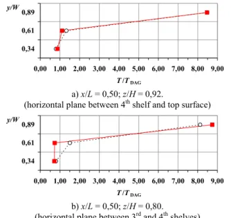
The validation of the numerical predictions results on the global performance characteristics of the display cabinet 3D model is accomplished by its comparison with experimental measurements data. Figures 3 to 4 present the comparative non dimensional profiles, for different planes, of the experimental average values of air temperature and numerical predictions. Figure 3 presents the non dimensional temperature profiles (by DAG temperature) obtained by the intersection between the vertical mid section plane with two horizontal planes. Figure 4 presents the non dimensional temperature profiles (by average temperature values along length) along the length of the equipment. Analyzing the compared values, the predicted steady state air flow and heat transfer inside the refrigerated display cabinet present both a reasonable agreement. The experimental average points are represented by { and the numerical predictions points are represented by .
The numerical predictions present a reasonable quantitative agreement and a qualitative similar tendency, being the highest quantitative discrepancy in the proximity of the air curtain. Considering the scale of the air temperature and velocity variations measured during the experimental testing, the global average relative deviation between the experimental data and numerical predictions of air temperature and velocity are acceptable in engineering situations. The non-overlapping of the results (experimental and numerical) is due to experimental errors (measurements precision, physical phenomena perturbation, etc) and computational model assumptions (steady state, turbulence model, boundary conditions definition, etc). Nevertheless, the combined analysis of the experimental and numerical results shows that the CFD model generally follows the pattern of the physical phenomena occurring in the real equipment.
a) x/L = 0,50; z/H = 0,92.
(horizontal plane between 4th shelf and top surface)
b) x/L = 0,50; z/H = 0,80.
(horizontal plane between 3rd and 4th shelves)
Figure 3. Non dimensional air temperature comparative profiles at the conservation space, T/TDAG (x/L = 0,50; y/W , z/H).
0,00 1,00 2,00 3,00 4,00 5,00 6,00 7,00 8,00 9,00 0,34 0,61 0,89 y/W T /TDAG 0,00 1,00 2,00 3,00 4,00 5,00 6,00 7,00 8,00 9,00 0,34 0,61 0,89 y/W T /TDAG
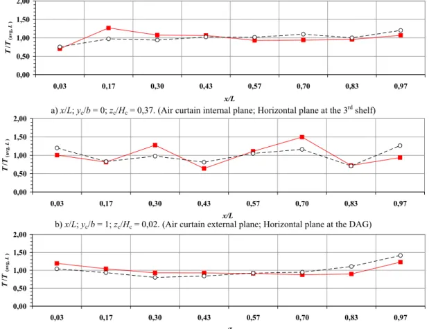
0,00 0,50 1,00 1,50 2,00 0,03 0,17 0,30 0,43 0,57 0,70 0,83 0,97 x/L T /T (avg , L )
a) x/L; yc/b = 0; zc/Hc = 0,37. (Air curtain internal plane; Horizontal plane at the 3rd shelf)
0,00 0,50 1,00 1,50 2,00 0,03 0,17 0,30 0,43 0,57 0,70 0,83 0,97 x/L T /T (avg , L )
b) x/L; yc/b = 1; zc/Hc = 0,02. (Air curtain external plane; Horizontal plane at the DAG)
0,00 0,50 1,00 1,50 2,00 0,03 0,17 0,30 0,43 0,57 0,70 0,83 0,97 x/L T /T (avg, L )
c) x/L; y/W = 0,68; z/H = 0,33. (Horizontal plane between well tray and 1st shelf)
Figure 4. Non dimensional air temperature, T/T(avg, L), comparative profiles at: (a-b) air curtain, (x/L; yc/b; zc/Hc), (c) between shelves, (x/L; y/W; z/H).
Temperature fields along y-z
Figure 5 presents the temperature maps for selected vertical planes along length. The ambient air has a parallel direction to the equipment’s frontal opening (along x). The temperature fields show the influence of the ambient air direction on the aerothermodynamic performance of the air curtain and on the air temperature distribution inside the conservation space. It is shown that the equipment’s end walls promote the air curtain instability and thus the thermal entrainment. The numerical predictions indicate higher refrigerated air losses to the exterior by the bottom part of the equipment near its physical extremities -Figure 5.a) and .d)- than near the mid section -Figure 5.b) and .c)-. At those locations, the air curtain instabilities are observed, being the most significant at the left side (x/L = 0,03), i.e., the side from the ambient air movement.
Temperature fields along x-y
Figure 6 presents the air temperature fields in x-y planes at different heights, since RAG (z/H = 0,38) to DAG (z/H = 0,92). The air temperature numerical predictions at the air curtain interface show the air curtain stability. The air curtain is well defined along length (x/L) near the DAG (z/H = 0,92).
Although, as the air curtain height increases (< z/H), it can be observed that the thermal entrainment increases near the end walls and across the air curtain. This means a reduction of the air curtain aerothermodynamic performance. The numerical results show a higher influence of the ambient air movement (from left to right) in the dimension of eddies structures located near the equipment’s end walls. The non uniformity of the refrigerated air temperature distribution along the spatial coordinates influences the food temperature differences depending on their location in the shelves.
Temperature fields along air curtain non dimensional width Figure 7 presents the air temperature fields for 3 planes along the non dimensional air curtain width: internal; medium; and external (yc/b = 0; = 0,5; = 1). These numerical results
show where the thermal entrainment is higher and how it spreads across the air curtain. It develops across the air curtain near the equipment’s end wall, and it is more significant at the left side where the ambient air comes. Even where the thermal entrainment is more pronounced, the aerothermodynamic blockage provided by the air curtain allows the reduction of the air temperature for half of its initial value (ambient air) in a linear dimension of 60 mm (DAG width, b).
a) x/L = 0,03. b) x/L = 0,30. c) x/L = 0,70. d) x/L = 0,97.
Figure 5. Air temperature field maps, T [ºC], along equipment’s non dimensional length, x/L.
a) z/H = 0,92. (horizontal plane between 4th shelf and DAG)
b) z/H = 0,66. (horizontal plane between 2sd and 3rd shelves)
c) z/H = 0,38. (horizon. plane between well tray and 1st shelf)
Figure 6. Air temperature field maps, T [ºC], along equipment’s non dimensional height, z/H.
In Figure 7 it can also be seen an increase of the thermal entrainment with the distance to the DAG (with z/H decrease). At the bottom part of the equipment, it can be observed a refrigerated air leakage to the exterior (Figure 7.c), which almost reaches to both sides at the exterior.
Mass and heat transfer rates
The regions that virtually limits the air curtain (yc/b = 0
and yc/b = 1) are divided into 30 control volumes each, as
presented in Figure 8, to evaluate the mass and heat transfer rates across the air curtain. It is considered a matrix structure with 5×6 rows×columns (n×m). For each control volume are determined the mass flow rate and the heat transfer rate by Equations 4 and 5. A v m& =ρ [kg s-1] (4) T C m Q&= & pΔ [W] (5)
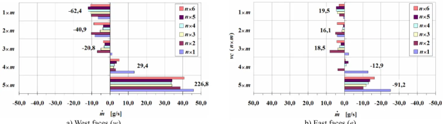
Figures 9 and 10 present the values and directions of the mass flow rate and heat transfer rate respectively, through the West and East faces of each control volume in which the air curtain is divided. The graphs are constructed in function of the rows’ matrix (n), corresponding to the air curtain heights. For each matrix row, are presented the mass flow rate and heat transfer values of the sections along the length of the frontal opening to the exterior, i.e., for the different columns of the matrix (m). Both the mass flow rate and heat transfer rate graphs contain the sum and respectively face values along length for each height section of the air curtain.
a) yc/b = 0. (Air curtain internal plane)
b) yc/b = 0,5. (Air curtain medium plane)
c) yc/b = 1. (Air curtain external plane)
Figure 7. Air temperature field maps, T [ºC], along non dimensional air curtain width, yc/b.
The numerical results show that the air curtain “gains” thermal energy from the ambient and conservation region (Figure 10). The former gains are related to the ambient air infiltration, thermal radiation, illumination and heat conduction through the equipment’s walls. These thermal energy gains are more significant at the end walls of the equipment (symbols: and ).
The 3D CFD model allow detecting the influence of the ambient air velocity, vamb = 0,2 m/s, parallel to the equipment’s
frontal opening (from left: to right: ), in the distribution of the mass flow rate and heat transfer rate across the air curtain, and consequently in the thermal entrainment.
Figure 8. Subdivision of the air curtain virtual limits by control volumes.
The mass flow rate direction at the external border (East faces) presented in Figure 9, shows the ambient air entrance e consequently thermal energy gain at higher heights (East faces of 1×m, 2×m and 3×m control volumes). The opposite appears at the lower heights (East faces of 4×m and 5×m control volumes). Along length, the highest values of the mass flow rate occur near the end walls (East faces of n×1, n×2 and n×6 control volumes).
At the higher heights of the internal border (West faces), the mass flow rate is directed to the conservation space (West faces of 1×m, 2×m e 3×m control volumes), corresponding to a energy “loss” (Figure 10). The reverse situation occurs at the lower heights (West faces of 4×m and 5×m control volumes). Along length, it can be seen, higher values of the mass flow rate near the end walls.
The global analysis of the temperature fields and mass flow rate and heat transfer rate across the air curtain emphasizes the potentialities of the 3D CFD model, by the prediction capabilities of the 3D air flow effects near the equipment’s end walls, characterized by the formation of 3D vortex structures that affect the aerothermodynamic performance of the air curtain along the equipment’s length. These numerical results are in agreement with the experimental analysis based in the point measuring technique of the air temperature, relative humidity and velocity. The thermal entrainment is due to eddies formation near the DAG; to the vertical vortex near the lateral walls; and to the air curtain breaking as we approach the RAG.
a) West faces (w). b) East faces (e).
Figure 9. Mass flow rate at the West (internal border) and East (external border) faces of the air curtain control volumes.
a) West faces (w). b) East faces (e).
Figure 10. Heat transfer rate at the West (internal border) and East (external border) faces of the air curtain control volumes.
CONCLUSION
A 3D CFD model applied to an open display cabinet has been developed to simulate the air fluid flow and the heat transfer. The agreement between the numerical predictions and experimental results is adequate to engineering problems.
The characterization of the air flow and heat transfers allows the identification of equipment’s length impact in the thermal entrainment. The thermal entrainment downward the air curtain is very dependent of the eddies formation, developed by the shear layer interactions and is enhanced by the turbulence intensity at the initial region of the air curtain jet that triggers mixture. The momentum reduction decreases the air curtain stability. The numerical results analysis revealed high values of the thermal entrainment at the initial and final linear dimensions due to side wall effects. Ambient air movement (from left to right) influences and magnifies the extremity effects. These conditions will promote a non-uniform air temperature distribution inside the refrigerated display cabinet and influences the differences in the product temperature. Additionally, the ambient air movement affects the return air temperature and consequently the energy efficiency of the equipment.
NOMENCLATURE
General
A Area, [m2].
b Air curtain width, [m].
BC Boundary condition.
Cp Specific heat, [J kg-1 K-1].
Dh Hydraulic diameter, [m].
H Height, [m].
I Electrical current intensity, [A]. It Turbulence intensity, [%].
k Turbulent kinetic energy [m2 s-2].
L Length, [m].
m& Mass flow rate, [kg s-1]
p Pressure, [Pa].
q& Heat flux, [W m-2].
Q& Heat transfer rate, [W].
Re Reynolds Number.
S General source term.
T Temperature, [ºC].
U Global heat transfer coefficient, [W m-2 K-1].
v Average velocity, [m s-1].
W Width, [m].
Superscripts and subscripts amb Ambient. avg Average. bb Black body. c Air curtain. cons Conservation. DAG Discharge air grille. evap Evaporator.
e, w Control volume faces (East, West). RAG Return air grille.
Greek Symbols
α Linear relaxation factor. ρ Density, [kg m-3].
ε Dissipation rate of k, [m2 s-3], Emissivity.
φ Relative humidity, [%]; General variable. μ Dynamic viscosity, [kg m-1 s-1]. Γ Diffusion coefficient. σ Standard deviation. σ2 Variance. λ Convergence criterion. ΔT Temperature difference. ACKNOWLEDGMENTS
The authors wish to acknowledge the support of University of Beira Interior – Electromechanical Engineering Department and of the refrigerated display cabinet manufacturer JORDÃO Cooling Systems®, Guimarães, Portugal (www.jordao.com).
REFERENCES
[1] Gaspar, P.D., Gonçalves, L.C.C, Pitarma, R.A., 2007. Estudo experimental do impacto da variação das condições do ar ambiente no desempenho global de expositores refrigerados abertos. Proc. of Engenharia ‘2007 – Inovação e Desenvolvimento. University of Beira Interior, Covilhã, Portugal (in Portuguese - PT).
[2] Faramarzi, R., 1999. Efficient display case refrigeration. ASHRAE Journal 41(11).
[3] Gray, I. et al., 2007. Improvement of air distribution in refrigerated vertical open front remote supermarket display cases, Int. J. Refrigeration, doi:10.1016/j.ijrefrig.2007.09.005.
[4] D’Agaro, P, Cortella, G., Croce, G., 2006. Two- and three-dimensional CFD applied to vertical display cabinets refrigeration. Int. J. Refrigeration 29(2), 178-190.
[5] ASHRAE. 2006. ASHRAE Handbook: Applications. ASHRAE. [6] Navaz, H K, Dabiri, D, Amin, M., Faramarzi, R., 2005. Past, present, and future research toward air curtain performance optimization. ASHRAE Trans. 111(1).
[7] Neto, L.P.C., Gameiro Silva, M.C., Costa, J.J., 2006. On the use of infrared thermography in studies with air curtain devices. Energy and Buildings 38(10), 1194-1199.
[8] Bhattacharjee, P., Loth, E., 2004. Simulations of laminar and transitional cold wall jets. Int. J. of Heat and Fluid Flow 25(1), 32-43. [9] Chen, Y.-G., Yuan, X.-L., 2005. Simulation of a cavity insulated by a vertical single band cold air curtain. Energy, Conversion & Management 46(11-12), 1745-1756.
[10] Field, B.S., Loth, E., 2006. Entrainment of refrigerated air curtains down a wall. Exp. Thermal and Fluid Science 30(3), 175-184. [11] Foster, A.M., Swain M.J., Barrett, R., et al, 2006. Effectiveness and optimum jet velocity for a plane jet air curtain used to restrict cold room infiltration. Int. J. Refrigeration 29(5), 692-699.
[12] Costa, J.J., Oliveira, L.A., Silva, M.C.G., 2006. Energy savings by aerodynamic sealing with a downward-blowing plane air curtain - A numerical approach. Energy and Buildings 38(10), 1182-1193. [13] European Standard EN 441. 1998. Refrigerated display cabinets, parts 1 to 12. European Comittee for Standardization.
[14] Gaspar, P.D., Gonçalves, L.C.C., Pitarma, R.A., 2006. Influência da ventilação no desempenho térmico e energético de expositores refrigerados. Proc. of ENVent, Cenertec, Espinho, Portugal (in PT) [15] Gaspar, P.D., Gonçalves, L.C.C, Pitarma, R.A., 2007. Experimental analysis of the thermal entrainment three dimensional effects in re-circulated air curtains. Proc. of 10th Int. Conf. on Air
Distribuition in Rooms – ROOMVENT 2007, Helsinki, Finland. [16] Smale, N.J., Moureh, J., Cortella, G., 2006. A review of numerical models of airflow in refrigerated food applications. Int. J. Refrigeration 29(6), 911-930.
[17] Norton, T, Sun, D.-W., 2006. CFD-an effective and efficient design and analysis tool for the food industry: a review. Trends in Food Science & Technology. 17(11), 600-620.
[18] Cortellla, G., Manzan, M. and Comini, G., 2001. CFD simulation of refrigerated display cabinets. Int. J. Refrigeration 24(3), 250-260. [19] Ge, Y.T., Tassou, S.A., 2001. Simulation of the performance of a single jet air curtains for vertical refrigerated display cabinets. Int. J. Refrigeration 21(2), 201–209.
[20] Navaz, H.K, Faramarzi, R., Gharib, M., Dabiri, D., Modarress, D., 2002. The application of advanced methods in analyzing the performance of the air curtain in a refrigerated display case. Trans. ASME J. Fluids Eng. 124, 756–764.
[21] Axell, M., Fahlén, P., 2003. Design criteria for energy efficient vertical air curtains in display cabinets. Proc. of 21st IIR Int. Congress of Refrigeration, Washington DC, U.S.A.
[22] Navaz, H.K., Henderson, B.S., Faramarzi, R., Pourmovahed, A., Taugwalder, F., 2005.Jet entrainment rate in air curtain of open refrigerated display cases. Int. J. Refrigeration 28(2), 267-275. [23] Foster, A.M., Madge, M., Evans, J.A., 2005. The use of CFD to improve the performance of a chilled multi-deck retail display cabinet. Int. J. Refrigeration 28(5), 698-705.
[24] Chen, Y.-G., Yuan, X.-L., 2005. Experimental study of the performance of single-band air curtains for multi-deck refrigerated display cabinet. J. Food Engineering 69(3), 261-267.
[25] Ferziger, J.H., Perić, M., 2002. Computational methods for fluid dynamics – 3rd edition, Springer-Verlag, Berlin, Germany.
[26] Yakhot, V., Orszag, S.A., 1986. Renormalization Group Analysis of Turbulence: I. Basic Theory. J. of Scientific Computing 1(1). [27] Rodi, W., 1980. Turbulence models and their application in hydraulics. A state of the art review. International Association for Hydraulics Research.
[28] Launder, B.E., Spalding, D.B., 1974. The numerical computation of turbulent flows. Computer Methods in Applied Mechanics and Engineering (3).
[29] Issa, R.I., 1985. Solution of the implicitly discretized fluid flow equations by operator-splitting. J. Computational Physics 62.
[30] Patankar, S.V., 1980. Numerical Heat Transfer and Fluid Flow. Hemisphere Publishing Corporation.
[31] Jang, D.S., Jetly, R., Acharya, S., 1986. Comparison of the PISO, SIMPLER, and SIMPLEC algorithms for the treatment of the pressure-velocity coupling in steady flow problems. Numerical Heat Transfer 10.
[32] Van Leer, B., 1979. Toward the ultimate conservative difference scheme, IV, a second order sequel to Godunov's method. J. of Computational Physics 32.
![Figure 5. Air temperature field maps, T [ºC], along equipment’s non dimensional length, x/L](https://thumb-eu.123doks.com/thumbv2/123dok_br/19174096.942444/8.892.64.823.155.466/figure-air-temperature-field-along-equipment-dimensional-length.webp)
![Figure 7. Air temperature field maps, T [ºC], along non dimensional air curtain width, y c /b](https://thumb-eu.123doks.com/thumbv2/123dok_br/19174096.942444/9.892.81.426.138.914/figure-air-temperature-field-maps-dimensional-curtain-width.webp)