EERI
Economics and Econometrics Research Institute
EERI Research Paper Series No 33/2010
ISSN: 2031-4892
A quantitative approach to the effects of social policy
measures. An application to Portugal, using Social
Accounting Matrices
Susana Santos
EERI
Economics and Econometrics Research Institute
Avenue de Beaulieu 1160 Brussels Belgium
A quantitative approach to the effects of
social policy measures. An application to
Portugal, using Social Accounting
Matrices
Susana Santos
ISEG (School of Economics and Management), TULisboa –
Technical University of Lisbon, UECE – Research Unit on
Complexity and Economics
9. July 2010
An application to Portugal, using Social Accounting Matrices. (*)
Susana Santos
ISEG (School of Economics and Management)/TULisboa – Technical University of Lisbon; UECE – Research Unit on Complexity and Economics (**) and DE – Department of Economics;
ssantos@iseg.utl.pt; https://aquila1.iseg.utl.pt/aquila/homepage/f645
(July 2010)
Abstract
The impacts of policy measures on transfers between government and households will be quantified using Social Accounting Matrices (SAMs).
The System of National Accounts (SNA) will be the main source used for the construction of the numerical version of these matrices, which will then form the basis for two algebraic versions. One version will consist of accounting multipliers, and structural path analysis will also be used
for its decomposition. The other version will be a so-called SAM-based linear model, in which each cell will be defined with a linear equation or system of equations, whose components will be all the known and quantified transactions of the SNA, using the parameters deduced from the numerical SAM that served as the basis for this model.
Macroeconomic aggregates and balances, as well as structural indicators of the distribution and use of income, will be calculated from numerical and algebraic versions of the SAM. These will make it possible to quantify and compare the effects of social policy measures and to evaluate their differences, in order to define the path for future research work on the SAM-based linear model.
Keywords: Social Accounting Matrix; SAM-based Modelling; Macroeconomic Modelling; Policy Analysis; Structural Path Analysis
JEL Codes: E61; E10; D57.
(*) Presented to the 18th International Input-Output Conference, held in Sydney, Australia, on 20-25/6/2010.
Abbreviations
CPA – Classification of Products by Activity
ESA 95 – European System of National and Regional Accounts in the European Community of 1995 (Eurostat, 1996)
GDP – Gross Domestic Product
INE – Instituto Nacional de Estatística (Statistics Portugal)
ISCED – International Standard Classification of Education
ISWGNA – Inter-Secretariat Working Group, published by the United Nations Statistical Office
NACE (Rev.1) – New Statistical Nomenclature of the Economic Activities in the European Community
NPISHs – Non-Profit Institutions Serving Households
SAM – Social Accounting Matrix
SNA – System of National Accounts
SNA 93 – System of National Accounts of 1993 (ISWG, 1993)
1. Introduction ... 1
2. The SAM numerical version ... 2
2.1. Structural indicators of the distribution and use of income; identifying social policy measures and the corresponding scenarios to be studied ... 12
3. The SAM algebraic versions ... 18
3.1. Accounting multipliers, their components and the first results for the scenarios identified ... 19
3.2. The SAM-based linear model ... 31
3.3. Accounting multipliers and the SAM-based linear model ... 36
4. Quantifying effects of social policy measures using macroeconomic aggregates and balances ... 36
5. Concluding Remarks ... 42
References ... 46
Appendices A.1. Accounting multipliers for Portugal in 1995 and 2005 ... 48
A.2. SAM-based linear model ... 58
A.2.1. Structural indicators ... 58
A.2.2. Macroeconomic aggregates ... 58
A.2.3. Conventions and declarations ... 58
1. Portuguese basic SAM (Social Accounting Matrix) for 1995 (in millions of euros) ... 4
2. Portuguese basic SAM (Social Accounting Matrix) for 2005 (in millions of euros) ... 5
3. Identifying the National Accounts transactions in the cells of the basic SAM ... 6
4. Portuguese SAM (Social Accounting Matrix) for 1995 (in millions of euros) ... 8
5. Portuguese SAM (Social Accounting Matrix) for 2005 (in millions of euros) ... 10
6. Distribution of the generated income, among factors of production and institutions, in the Portuguese SAM for 1995 and 2005 (in percentage terms) ... 12
7. Distribution and use of disposable income, among institutions, in the Portuguese SAM for 1995 and 2005 (in percentage terms) ... 13
8. Per capita household disposable income and final consumption (euros per person), in Portugal in 1995 and 2005 ... 15
9. Current taxes on income, wealth, etc., paid by households to the government, and social benefits other than social transfers in kind paid, by the government to households, in Portugal in 1995 and 2005 ... 15
10.The Government and Households Budgets in the Portuguese SAM for 1995 and 2005 (in millions of euros) ... 17
11.The SAM in endogenous and exogenous accounts ... 19
12.Direct influences of unitary changes in the exogenous current receipts of the government . 23 13.Global influences of unitary changes in the exogenous current receipts of the government ... 24
14.Additional group influences of unitary changes in the exogenous current receipts of the government ... 24
15.Structural path analysis of the global influences on aggregate demand of unitary changes in the exogenous current receipts of the government ... 27
16.Direct influences of unitary changes in the exogenous current receipts of households ... 28
17.Global influences of unitary changes in the exogenous current receipts of households ... 28
18.Additional group influences of unitary changes in the exogenous current receipts of households ... 29
19.Structural path analysis of the global influences on aggregate demand of unitary changes in the exogenous current receipts of households ... 31
20.The formalized transactions (cells) in the basic SAM ... 32
government on macroeconomic balances in 1995 and 2005 ... 39
23.Impacts of an increase (of 1%) in the social benefits other than social transfers in kind received by households from the government on macroeconomic aggregates in 1995 and 2005 ... 41
24.Impacts of an increase (of 1%) in the social benefits other than social transfers in kind received by households from the government the macroeconomic balances in 1995 and 2005 ... 41
Appendix A.1. Accounting multipliers for Portugal in 1995 and 2005 A.1.1. Average expenditure propensities matrices – 1995 (Scenario A) ... 48
A.1.2. Average expenditure propensities matrices – 2005 (Scenario A) ... 48
A.1.3. Accounting multipliers matrix – 1995 (Scenario A) ... 49
A.1.4. Accounting multipliers matrix – 2005 (Scenario A) ... 49
A.1.5. Additional intragroup or direct effects matrix (M1 - I) – 1995 (Scenario A) ... 50
A.1.6. Additional intragroup or direct effects matrix (M1 - I) – 2005 (Scenario A) ... 50
A.1.7. Additional intergroup or indirect effects matrix (M2 - I) * M1 – 1995 (Scenario A) ... 51
A.1.8. Additional intergroup or indirect effects matrix (M2 - I) * M1 – 2005 (Scenario A) ... 51
A.1.9. Additional extragroup or cross effects matrix (M3 - I) * M2* M1- 1995 (Scenario A) .... 52
A.1.10.Additional extragroup or cross effects matrix (M3 - I) * M2* M1- 2005 (Scenario A) .... 52
A.1.11.Average expenditure propensities matrices – 1995 (Scenario B) ... 53
A.1.12.Average expenditure propensities matrices – 2005 (Scenario B) ... 53
A.1.13.Accounting multipliers matrix – 1995 (Scenario B) ... 54
A.1.14.Accounting multipliers matrix – 2005 (Scenario B) ... 54
A.1.15.Additional intragroup or direct effects matrix (M1 - I) – 1995 (Scenario B) ... 55
A.1.16.Additional intragroup or direct effects matrix (M1 - I) – 2005 (Scenario B) ... 55
A.1.17.Additional intergroup or indirect effects matrix (M2 - I) * M1 – 1995 (Scenario B) ... 56
A.1.18. Additional intergroup or indirect effects matrix (M2 - I) * M1 – 2005 (Scenario B ... 56
A.1.19.Additional extragroup or cross effects matrix (M3 - I) * M2* M1- 1995 (Scenario B) .... 57
A.1.20.Additional extragroup or cross effects matrix (M3 - I) * M2* M1- 2005 (Scenario B) .... 57
Appendix A.3. Portuguese Integrated Economic Accounts A.3.1. 1995 (in millions of euros) ... 65
1. Introduction
This paper is intended to be yet one more (small) step forward in the research that its author has been undertaking, for several years, into the SAM in general and now, in particular, into SAM-based modelling. Thus, on the one hand, it uses the work published in Santos (2008, 2009, 2009a) and the papers prepared for presentation by the author at two conferences in 20092 and, on the other hand, it updates almost all of that work to 2005.
From the author’s point of view, the SAM is a powerful working instrument for socio-(macro)economic planning, since with its underlying methodology it is possible to arrive at perfectly harmonized models and databases that contemplate important aspects of the economic and social sides of the real world. Further research is planned to improve this part of the work and to study other aspects of these (economic and social) sides, as well as to consider yet further issues (such as the environment, for instance).
In the Preface to the study by F. Lequiller and D. Blades, entitled Understanding National Accounts, E. Giovannini says: “today’s national accounts are the core of a modern system of
economic statistics, and provide the conceptual and actual tool to bring to coherence hundreds of statistical sources available in developed countries”3. This is, in fact, a particular advantage enjoyed by developed countries and something which the developing countries are gradually working towards.
Thus, working with SAMs constructed from the national accounts can be a way of working with quantified reality in a more precise fashion. It is in this particular area that the author has been researching, constructing numerical (macro)SAMs from the national accounts (Section 2) and developing a SAM-based linear model. In the latter case, each cell is defined through a linear equation or system of equations, whose components are all the known and quantified transactions of the national accounts, using the parameters deduced from the numerical SAM that served as the basis for this model (Section 3.2). Such a model still has very restrictive assumptions, but its purpose is to better understand the results obtained and to progressively improve them. In order to achieve this aim, another SAM-based model will also be used – the
2 "Constructing and Modelling SAMs from the SNA for the study of impacts of policy measures" (57th Session of
the International Statistical Institute). Durban (South Africa): 16-22/8/2009.
"SAM-based modelling for policy and scenario analysis" (17th International Input-Output Conference, promoted by
IIOA (International Input-Output Association) and the Department of Economics of the School of Economics,
Business and Accountancy of the University of São Paulo). São Paulo (Brazil): 13-17/7/2009.
one based on accounting multipliers4 – whose additive decomposition will be analysed before the use of structural path analysis (Section 3.1) in order to provide a better understanding and interpretation of the differences between the results (Sections 3.3 and 4).
Therefore, in order to study the distributional effects of social policy measures, after analysing some of the structural indicators of the distribution and use of income and identifying the transfers between government and households that are to be worked upon as social policy measures (Section 2.1), identical experiments to those of the work referred to in the first paragraph will be performed using the two above-mentioned SAM-based models or SAM algebraic versions – multipliers and linear model. The analysis of the results and their comparison will be conducted using macroeconomic aggregates and balances (Section 4).
The concluding remarks (Section 5) will highlight not only the main methodological aspects of the work, but also the main results and their differences, in accordance with the alternative applications of the models to Portugal in two years separated by a gap of eleven years – 1995 and 2005. Finally, some guidelines will be provided suggesting a possible path for future research work on the SAM-based linear model.
2. The SAM numerical version
As mentioned above, the national accounts will be the source of information adopted in this work.
The System of National Accounts (SNA) that provided the information worked on for Portugal in 1995 and 2005 was the European System of National and Regional Accounts in the European Community of 1995 – ESA 95 (Eurostat, 1996), which is based on the 1993 version of the International United Nations System of National Accounts – SNA 93, prepared by the Inter-Secretariat Working Group and published by the United Nations Statistical Office (ISWGNA, 1993). Consequently, all the conventions and nomenclatures of that system have been adopted. Considering the purpose of this paper and the information available for the years to be studied, the classification adopted for the accounts of both the numerical and, consequently, the algebraic versions of the SAM does not involve too high a level of disaggregation. Thus, in the case of the domestic economy, “Production and Trade” was divided into six groups of products and
activities5 and two factors of production – labour (employees) and own assets (employers and/or own account workers and capital). In turn, “Institutions” were divided into current, capital and financial accounts, with the last of these being a totally aggregate figure (due to the lack of information on the “from whom to whom” transactions) while the others were divided into: households, enterprises (or non-financial corporations), financial corporations, general government and non-profit institutions serving households (NPISH). Besides these accounts, we also have an aggregate account for the “rest of the world”.
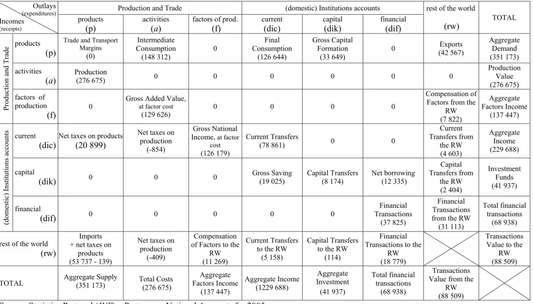
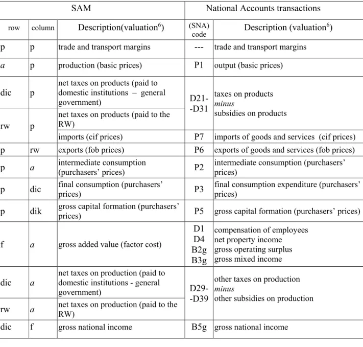
The criterion used by the author for ordering the accounts was the one underlying the SAMs represented in Tables1, 2, 4 and 5 – the first two presented in a basic and completely aggregate form and the others presented with the adopted disaggregation. Table 3 identifies the SNA transactions in the cells of the basic SAM, which will maintain their characteristics after the adopted disaggregation.
Table 1. Portuguese basic SAM (Social Accounting Matrix) for 1995 (in millions of euros)
Outlays (expenditures) Incomes
(receipts)
Production and Trade (domestic) Institutions accounts rest of the world
(rw) TOTAL
products
(p) activities (a)
factors of prod.
(f) current (dic) capital (dik) financial (dif)
Pr odu ction an d Tr ad
e products
(p)
Trade and Transport Margins
(0)
Intermediate Consumption
(84 102) 0
Final Consumption
(64 898)
Gross Capital Formation
(19 623) 0
Exports (24 433) Aggregate Demand (193 056) activities
(a)
Production
(154 394) 0 0 0 0 0 0
Production Value (154 394) factors of
production
(f) 0
Gross Added Value, at factor cost
(70 725) 0 0 0 0
Compensation of Factors from the
RW (3 243) Aggregate Factors Income (73 968) (d omestic) In stitu tio ns acco un ts current
(dic)Net taxes on products (10 283 )
Net taxes on production
(-346)
Gross National Income, at factor cost
(70 542)
Current Transfers
(42 145) 0 0
Current Transfers from the RW (3 960) Aggregate Income (126 583) capital
(dik) 0 0 0 Gross Saving (17 291) Capital Transfers (4930) Net borrowing (40)
Capital Transfers from the RW (2 320) Investment Funds (24 582) financial
(dif) 0 0 0 0 0
Financial Transactions
(35 030)
Financial Transactions from the RW
(9 257)
Total financial transactions
(44 287)
rest of the world (rw)
Imports + net taxes on
products (28 127 + 252)
Net taxes on production
(-87)
Compensation of Factors to the
RW (3 426)
Current Transfers to the RW
(2 249)
Capital Transfers to the RW
(29)
Financial Transactions to the
RW (9 217)
Transactions Value to the
RW (43 213)
TOTAL Aggregate Supply (193 056) Total Costs (154 394) Factors Income Aggregate (73 968) Aggregate Income (126 583) Aggregate Investment (24 582) Total financial transactions (44 287) Transactions Value from the
RW (43 213)
Table 2. Portuguese basic SAM (Social Accounting Matrix) for 2005 (in millions of euros)
Outlays (expenditures) Incomes
(receipts)
Production and Trade (domestic) Institutions accounts rest of the world
(rw) TOTAL
products
(p) activities (a)
factors of prod.
(f) current (dic) capital (dik) financial (dif)
Pr odu ction an d Tr ad
e products
(p)
Trade and Transport Margins
(0)
Intermediate Consumption
(148 312) 0
Final Consumption
(126 644)
Gross Capital Formation
(33 649) 0
Exports (42 567) Aggregate Demand (351 173) activities
(a)
Production
(276 675) 0 0 0 0 0 0
Production Value (276 675) factors of
production
(f) 0
Gross Added Value, at factor cost
(129 626) 0 0 0 0
Compensation of Factors from the
RW (7 822) Aggregate Factors Income (137 447) (do m estic) In stitu tio ns accou nts current
(dic)Net taxes on products (20 899)
Net taxes on production
(-854)
Gross National Income, at factor
cost (126 179)
Current Transfers
(78 861) 0 0
Current Transfers from the RW (4 603) Aggregate Income (229 688) capital
(dik) 0 0 0 Gross Saving (19 025) Capital Transfers (8 174) Net borrowing (12 335)
Capital Transfers from the RW (2 404) Investment Funds (41 937) financial
(dif) 0 0 0 0 0
Financial Transactions
(37 825)
Financial Transactions from the RW
(31 113)
Total financial transactions
(68 938)
rest of the world (rw)
Imports + net taxes on
products (53 737 - 139)
Net taxes on production
(-409)
Compensation of Factors to the
RW (11 269)
Current Transfers to the RW
(5 158)
Capital Transfers to the RW
(114)
Financial Transactions to the
RW (18 779)
Transactions Value to the
RW (88 509)
TOTAL Aggregate Supply (351 173) Total Costs (276 675) Factors Income Aggregate (137 447) Aggregate Income (1229 688) Aggregate Investment (41 937) Total financial transactions (68 938) Transactions Value from the
RW (88 509)
Table 3. Identifying the National Accounts transactions in the cells of the basic SAM
SAM National Accounts transactions
row column Description(valuation6) (SNA)
code Description (valuation6)
p p trade and transport margins --- trade and transport margins
a p production (basic prices) P1 output (basic prices)
dic p net taxes on products (paid to domestic institutions – general
government) D21-
-D31
taxes on products
minus
subsidies on products
rw p net taxes on products (paid to the RW)
imports (cif prices) P7 imports of goods and services (cif prices)
p rw exports (fob prices) P6 exports of goods and services (fob prices)
p a intermediate consumption (purchasers’ prices) P2 intermediate consumption (purchasers’ prices)
p dic final consumption (purchasers’ prices) P3 final consumption expenditure (purchasers’ prices)
p dik gross capital formation (purchasers’ prices) P5 gross capital formation (purchasers’ prices)
f a gross added value (factor cost)
D1 D4 B2g B3g
compensation of employees net property income
gross operating surplus gross mixed income
dic a
net taxes on production (paid to domestic institutions - general
government) D29-
-D39
other taxes on production
minus
other subsidies on production
rw a net taxes on production (paid to the RW)
dic f gross national income B5g gross national income
6 In the transactions involving products and/or activities, three levels of valuation can be distinguished: factor cost; basic/cif/fob prices and purchasers’ or market prices.
The first of these levels is that of the compensation of the factors used in the production process of the domestic economy during the accounting period. In analysing those factors, one can distinguish between labour (employees and own-account workers and/or employers) and capital. In this case, compensation is respectively the compensation of employees (wages and salaries and employers’ social contributions – transactions D11 and D12 of the National Accounts), mixed income (balance B3 of the National Accounts) and the gross operating surplus (balance B2 of the National Accounts).
At the second level, one can distinguish between the production of the domestic economy and imports. In the first case, this is measured by the factor cost from the previous level, plus (other) taxes on production (transaction D29 of the National Account), net of subsidies on production (transaction D39 of the National Accounts), as well as by intermediate consumption. This represents the basic price level of the (domestic) production that will be transacted in the domestic market and the fob (free on board) price level of the production that will be exported. Imports, valued at cif (cost-insurance-freight included) prices, are added, at this level, to the above-mentioned unexported part of domestic production that will be transacted in the domestic market.
SAM National Accounts transactions
row column Description(valuation6) (SNA)
code Description (valuation6)
rw f compensation of factors to the RW
D1 D4
primary income paid to/received from the rest of the world
compensation of employees net property income
f rw compensation of factors from the RW
dic dic current transfers within domestic institutions D5 D6 D7 D8
current taxes on income, wealth, etc. social contributions and benefits other current transfers
adjustment for the change in the net equity of households in pension funds reserves
rw dic current transfers to the RW
dic rw current transfers from the RW
dik dic gross saving B8g gross saving
dik dik capital transfers within domestic institutions
D9 capital transfers
dik rw capital transfers from the RW
rw dik capital transfers to the RW
dik dif - net borrowing7 B9 net borrowing
dif dif financial transactions within domestic institutions F1 F2 F3 F4 F5 F6 F7
monetary gold and special drawing rights (SDRs)
currency and deposits securities other than shares loans
shares and other equity insurance technical reserves other accounts receivable/payable
rw dif financial transactions to the RW
dif rw financial transactions from the RW
Source: Santos (2007a).
Note: See the correspondence identified between this Table and the values (in brackets) of the basic SAMs (Tables 1 and 2) in the “Portuguese Integrated Economic Accounts for Portugal in 1995 and 2005” – Tables A.3.1 and A.3.2. (Appendix A.3.)
Details on the sources of information and methodologies used in the construction of the SAM for 1995 (with a higher level of disaggregation) can be found in Santos, 2009: 179-184 – identical to those adopted in the SAM for 2005.
7 In the National Accounts, the net lending (+) or borrowing (-) of the total economy is the sum of the net lending or borrowing of the institutional sectors. It represents the net resources that the total economy makes available to the rest of the world (if it is positive) or receives from the rest of the world (if it is negative). The net lending (+) or borrowing (-) of the total economy is equal (but with an opposite mathematical sign) to the net borrowing (-) or lending (+) of the rest of the world (SEC 95, Prg. 8.98).
Table 4. Portuguese SAM (Social Accounting Matrix) for 1995 (in millions of euros)
Table 4. Portuguese SAM (Social Accounting Matrix) for 1995 (in millions of euros) (continued)
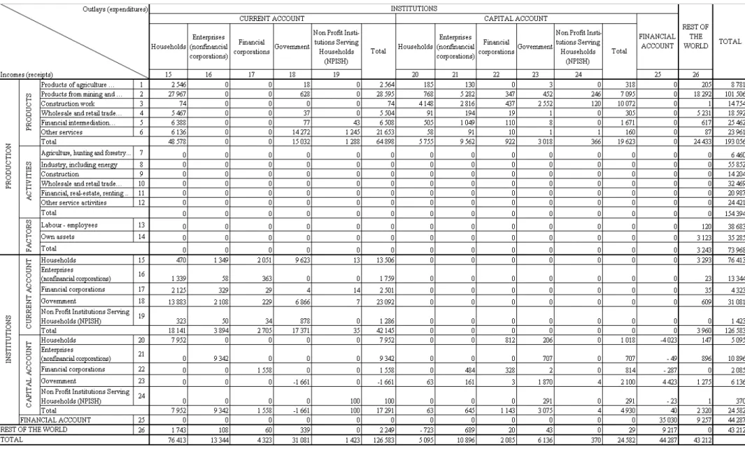
Table 5. Portuguese SAM (Social Accounting Matrix) for 2005 (in millions of euros)
Table 5. Portuguese SAM (Social Accounting Matrix) for 2005 (in millions of euros) (continued)
2.1. Structural indicators of the distribution and use of income; identifying social policy measures and the corresponding scenarios to be studied
Some indicators were calculated in order to be able to better identify the distributional effects of social policy measures. Thus, structural indicators of the functional and institutional distribution of generated income, as well as of the use of disposable income were calculated from the numerical version of the SAM for the two years under study – without any additional data8. Since additional data were worked on in a previous study for 1995 (Santos, 2009), some details will be used from this work in order to complement the following analysis.
Table 6. Distribution of the generated income, among factors of production and institutions, in the Portuguese SAM for 1995 and 2005 (in percentage terms).
1995 2005
Factors of Production
(generated income = gross added value, at factor cost)
Labour
(employees) 54.5 58.1
Own assets
(employers and/or own-account workers; capital) 45.5 41.9
Total 100.0 100.0
Institutions
(generated income = gross national income)
Households 84.5 84.2
Non-financial corporations 16.4 11.9
Financial corporations 2.5 3.7
General government -3.6 -0.6
Non-profit institutions serving households 0.2 0.8
Total 100.0 100.0
Sources: Tables 4 and 5.
In the functional distribution of the generated income, or the distribution of the gross added value among factors of production (see the first part of Table 6), a little more than half is compensation of employees, which in 2005 was 3.6 percentage points higher than in 1995. In 1995, the level of education of employees was as follows9: 48.3%, lower; 33%, medium; 18.7%, higher. In turn, employers and/or own-account workers, whose compensation represented
8 In the case of the SAM-based linear models, these indicators can also be calculated from the algebraic version, with the equations described in Appendix A.2.1.
7.5% of the 45.5% generated by own assets, were distributed according to the following levels of education: 55.7%, lower; 33.3%, medium; 11%, higher (Santos, 2009: 92-93).
In terms of institutional distribution (see the second part of Table 6), households have the most significant share of the generated income, which was slightly less in 2005. At a significant distance from households, non-financial corporations were in second position, although their importance declined from 1995 to 2005, in favour of all the others. Attention should be drawn to the position of the general government and the decrease in its negative value in 2005, meaning that its contribution to generated income increased significantly.
In 1995, considering their main source of income, within the 84.5% of the generated income of households, 62.1% came from employees (with wages and salaries as the main source of income) and 18.6% from employers and/or own-account workers (with mixed income including property income as the main source of income) (Santos, 2009: 96).
Each institution obtains its disposable income by excluding from gross national income the current transfers paid to other institutions and to the rest of the world, and by including the current transfers received from the other institutions and the rest of the world and, in the case of the government, net indirect taxes. This disposable income is then used in final consumption and saved, except in the case of non-financial and financial corporations, which do not have any final consumption.
Table 7. Distribution and use of disposable income, among institutions, in the Portuguese SAM for 1995 and 2005 (in percentage terms).
Distribution of Disposable
Income
Use of Disposable Income Final
Consumption Saving
1995
Households 69.3 86.3 13.7
Non-financial corporations 11.2 0.0 100.0
Financial corporations 1.9 0.0 100.0
General government 16.0 112.4 -12.4
Non-profit institutions serving households 1.7 92.8 7.2
Total 100.0 79.3 20.7
2005
Households 69.9 90.8 9.2
Non-financial corporations 6.7 0.0 100.0
Distribution of Disposable
Income
Use of Disposable Income Final
Consumption Saving
General government 18.4 117.6 -17.6
Non-profit institutions serving households 2.2 90.9 9.1
Total 100.0 87.1 12.9
Sources: Tables 4 and 5.
As it would be of expecting, households have more than a half of the disposable income, followed by general government, with less than a quarter, having been both positions slightly reinforced in 2005 – the same happened with the other institutions, except the non-financial corporations.
As is to be expected, households have more than half of disposable income, followed by general government, with less than a quarter, with both positions having been slightly reinforced in 2005 – the same thing happened with other institutions, except non-financial corporations.
In 1995, within the 69.3% of the disposable income of households, the group whose main source of income was wages and salaries (employees) accounted for 41.9% (Santos, 2009: 98).
It should be noted that the final consumption considered here is the expenditure (transaction P3 of the national accounts) and not the “actual” final consumption (transaction P4 of the national accounts), i.e. the amount really spent by each institution, although a part of the final consumption of the general government and (all) that of the NPISH will take the form of social transfers in kind (transaction D63 of the national accounts) and will include the “actual” final consumption of households.
Final consumption expenditure absorbed the largest and an increasing (except for the NPISH) part of disposable income, in detriment to saving, whose share fell by 7.8 percentage points, from 1995 to 2005.
On the other hand, since, in this case, households represent everybody in Portugal, per capita
Table 8. Per capita household disposable income and final consumption (euros per person), in Portugal in 1995 and 2005.
Disposable income Final Consumption
Expenditure Actual
1995 5 761 4 837 5 850
2005 9 768 8 672 10 766
Source: Statistics Portugal (INE) – Portuguese National Accounts for 1995 and 2005; Statistical
Yearbook for Portugal - 2008.
Thus, on average, Portuguese people saw their per capita disposable income and final
consumption significantly increase over eleven years (disposable income: 69.6%; final consumption expenditure: 79.3%; actual final consumption: 84%). This also means a real improvement, since in 2005 the implicit price index in final consumption was 137.15 and in GDP 137.34 (1995 = 100)10. Information by groups of households would improve our knowledge about this evolution, although unfortunately this is not available.
Since the aim is to test methodologies designed to illustrate the distributional effects of social policy measures, which could have been the ones described above that were adopted for improving the financial situation of people – and therefore of households – we should consider flows in which both government and households intervene directly, for instance: direct taxes on income, paid by households to the government; and social benefits, paid by the government to households. Table 9 shows the absolute and relative positions of those flows in the years studied.
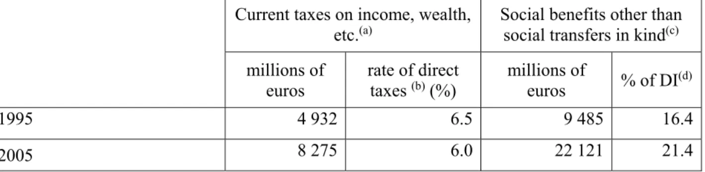
Table 9. Current taxes on income, wealth, etc., paid by households to the government, and social benefits other than social transfers in kind, paid by the government to households, in Portugal in 1995 and 2005.
Current taxes on income, wealth,
etc.(a) Social benefits other than social transfers in kind(c) millions of
euros rate of direct taxes (b) (%) millions of euros % of DI(d)
1995 4 932 6.5 9 485 16.4
2005 8 275 6.0 22 121 21.4
Source: Statistics Portugal (INE) – Portuguese National Accounts for 1995 and 2005.
Notes:
(a) Transaction D5 of the National Accounts.
(b) Current taxes on income, wealth, etc. paid by households to the government, per unit of received aggregate income11.
(c) Transaction D62 of the National Accounts12.
(d) Social benefits other than social transfers in kind paid by the government to households, per unit of disposable income of households.
These figures reveal a tendency, on the one hand, towards a decrease in the rate of direct taxes and, on the other hand, towards an increase in the social benefits, which, in a first approach, goes some way towards achieving the above-mentioned aim of improving the financial situation of people.
On the other hand, Table 10 helps us to see the position of these flows in the budgets of these two institutional sectors.
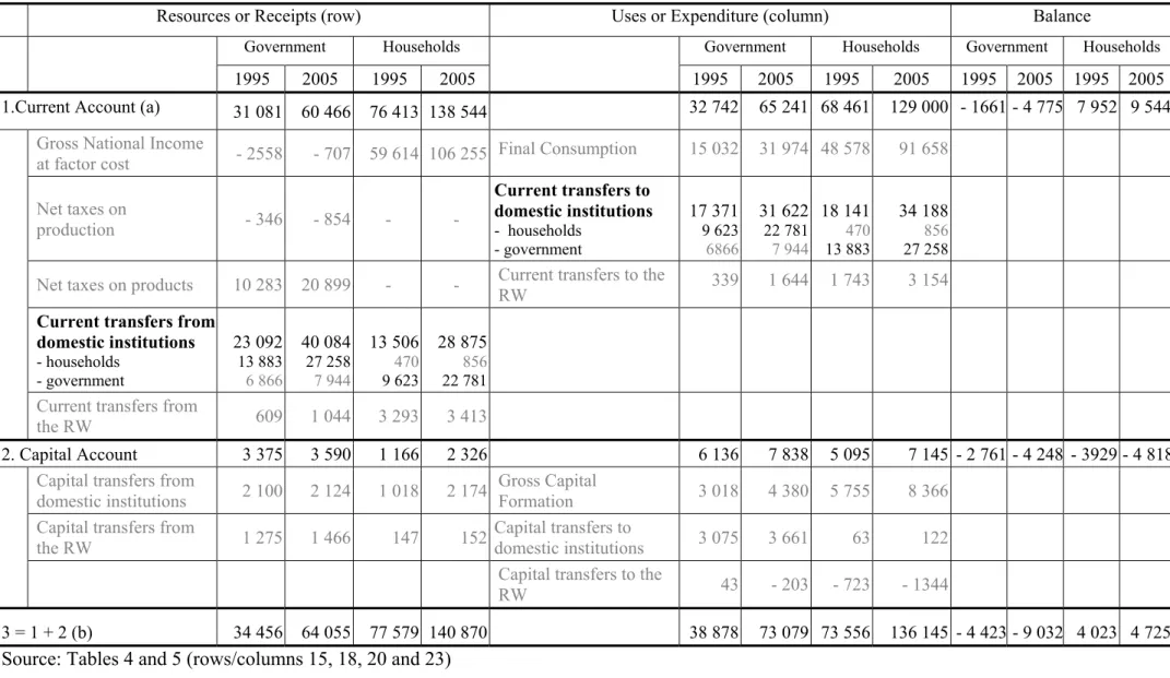
Table 10. The Government and Households Budgets in the Portuguese SAM for 1995 and 2005 (in millions of euros)
Resources or Receipts (row) Uses or Expenditure (column) Balance
Government Households Government Households Government Households
1995 2005 1995 2005 1995 2005 1995 2005 1995 2005 1995 2005 1.Current Account (a) 31 081 60 466 76 413 138 544 32 742 65 241 68 461 129 000 - 1661 - 4 775 7 952 9 544
Gross National Income
at factor cost - 2558 - 707 59 614 106 255 Final Consumption 15 032 31 974 48 578 91 658
Net taxes on
production - 346 - 854 - -
Current transfers to domestic institutions - households
- government 17 371 9 623 6866 31 622 22 781 7 944 18 141 470 13 883 34 188 856 27 258
Net taxes on products 10 283 20 899 - - Current transfers to the RW 339 1 644 1 743 3 154
Current transfers from domestic institutions - households - government 23 092 13 883 6 866 40 084 27 258 7 944 13 506 470 9 623 28 875 856 22 781
Current transfers from
the RW 609 1 044 3 293 3 413
2. Capital Account 3 375 3 590 1 166 2 326 6 136 7 838 5 095 7 145 - 2 761 - 4 248 - 3929 - 4 818
Capital transfers from
domestic institutions 2 100 2 124 1 018 2 174 Gross Capital Formation 3 018 4 380 5 755 8 366 Capital transfers from
the RW 1 275 1 466 147 152 Capital transfers to domestic institutions 3 075 3 661 63 122 Capital transfers to the
RW 43 - 203 - 723 - 1344
3 = 1 + 2 (b) 34 456 64 055 77 579 140 870 38 878 73 079 73 556 136 145 - 4 423 - 9 032 4 023 4 725
Source: Tables 4 and 5 (rows/columns 15, 18, 20 and 23) (a) Balance = Gross saving
Thus, in terms of the position of the current transfers in the flows of domestic institutions into the government and households’ budget in the years studied, the main sources of the government’s receipts are current transfers from domestic institutions (67% in 1995 and 62.6% in 2005) and net taxes on products, while the main sources of its expenditure are current transfers to domestic institutions (44.7% in 1995 and 43.3% in 2005) and final consumption, with expenditures being increasingly larger than receipts and leading to the corresponding increase of the deficit in all of its balances. In the case of households, which maintain positive current and total budget balances, the main sources of receipts and expenditures are, respectively, the (gross national) income generated by them and final consumption – with current transfers playing a less important role (17.4% in 1995 and 20.5% in 2005, in total receipts; 24.7% in 1995 and 25.1% in 2005, in total expenditures). Therefore it is to be expected that changes in the current transfers between the government and households will certainly have a greater impact on government budget than on the households’ budget.
For a better study of these effects, two scenarios will be studied: one (A) in which there will be a 1% reduction in the rate of the direct taxes associated with the current taxes on income, wealth, etc., paid by households to the government; and another (B) in which there will be a 1% increase in the social benefits (other than social transfers in kind) received by households from the government.
3. The SAM algebraic versions
Since our concern here is to quantify the effects of the social policy measures identified above, while also paying close attention to income distribution, the accounts of the institutions and their associated transactions will assume a central role. However, the production and rest of the world accounts should not be neglected, but their associated transactions must be afforded a level of specification that is different from the one found in models that attribute them a central role.
3.1. Accounting multipliers, their components and the first results for the scenarios identified
The base methodology that is to be followed is centred upon the use of multipliers and their decomposition. A systematic outline of this methodology is provided below, following Santos 2004 and 2007, in keeping with the work of Pyatt and Roe (1977), Pyatt and Round (1985) and Defourny and Thorbecke (1984).
a) Deduction of the accounting multipliers
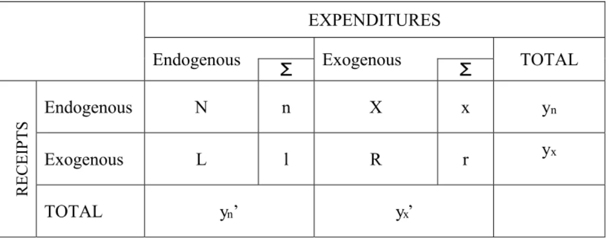
As shown in Table 11, we will have both exogenous and endogenous accounts, so that consequently the transactions in each cell of the SAM will be considered exogenous or endogenous according to the corresponding row and column accounts.
Table 11. The SAM in endogenous and exogenous accounts
EXPENDITURES
Endogenous
Σ
ExogenousΣ
TOTALRECEIPTS
Endogenous N n X x yn
Exogenous L l R r yx
TOTAL yn ’ yx’
Source: Pyatt and Round (1985).
where:
N = matrix of transactions between endogenous accounts; n = vector of the (corresponding) row sums.
X = matrix of transactions between exogenous and endogenous accounts (injections from first
into second); x = vector of the (corresponding) row sums.
L = matrix of transactions between endogenous and exogenous accounts (leakages from first into second); l = vector of the (corresponding) row sums.
R = matrix of transactions between exogenous accounts; r = vector of the (corresponding) row sums.
yn = vector (column) of the receipts of the endogenous accounts (ŷn: diagonal; ŷn-1: inverse); yn’ = vector (row) of the expenditures of the same accounts.
From Table 11, it can be written that
yn = n + x (1)
yx = l + r (2)
The amount that the endogenous accounts receive is equal to the amount that they spend (row totals equal column totals). In other words, in aggregate terms, total injections from the exogenous into the endogenous accounts (i.e. the column sum of “x”) are equal to total leakages from the endogenous into the exogenous accounts, i.e. considering i’ to be the unitary vector (row), the column sum of “1” is:
x * i’ = l * i’. (3)
In the structure of Table 11, if the entries in the N matrix are divided by the corresponding total expenditures
,
a corresponding matrix (squared) can be defined of the average expenditurepropensities of the endogenous accounts within the endogenous accounts or of the use of resources within those accounts. Calling this matrix An, it can be written that
An = N*ŷn -1 (4)
N = An*ŷn (5)
Considering equation (1), yn = An*yn + x (6)
Therefore, yn = (I-An)-1* x = Ma * x. (7)
We thus have the equation that gives the total receipts of the endogenous accounts (yn), by multiplying the injections “x” by the matrix of the accounting multipliers:
Ma = (I-An)-1. (8)
On the other hand, if the entries in the L matrix are divided by the corresponding total expenditures
,
a corresponding matrix (non squared) can be defined of the average expenditurepropensities of the endogenous accounts into the exogenous accounts or of the use of resources from the endogenous accounts into the exogenous accounts. Calling this matrix Al, it can be written that
Al = L*ŷn-1 (9)
L = Al*ŷn (10)
Considering equation (2), yx = Al*yn + r (11)
Thus, l = Al * yn = Al * (I-An)-1* x = Al * Ma * x. (12)
b) Decomposition of the accounting multipliers
Accounting multipliers can be decomposed if we consider the An matrix and two other ones with the same size (Bn - with the diagonal of An, whilst all the other elements are null - and Cn - with a null diagonal, but with all the other elements of An). In this way, it can be written that
An = Bn + Cn. (13)
Thus, from equation (6):
yn = Bn * yn +Cn * yn + x = I – (I - Bn)-1 *Cn-1 * (I - Bn)-1 * x 13. (14) Therefore: Ma = I – (I - Bn)-1 *Cn-1 * (I - Bn)-1 = M3*M2*M1. (15)
The accounting multiplier matrix is thus decomposed into multiplicative components, each of which relates to a particular kind of connection in the system as a whole (Stone, 1985)14.
- The intragroup or direct effects matrix, which represents the effects of the initial exogenous injection within the groups of accounts intowhich it had originally entered i.e.:
M1 = (I - Bn)-1. (16)
- The intergroup or indirect effects matrix, which represents the effects of the exogenous injection into the groups of accounts, after its repercussions have completed a tour through all the groups and returned to the one which they had originally entered In other words, if we consider “t” to be the number of groups of accounts (six in the present study):
M2 = {I - [(I - Bn)-1 * Cn ]t}-1. (17)
- The extragroup or cross effects matrix, which represents the effects of the exogenous injection when it has completed a tour outside its original group without returning to it, or, in other words, when it has moved around the whole system and ended up in one of the other groups. Thus, for the “t” groups of accounts:
M3 = {I + [(I - Bn)-1 * Cn ] + [(I - Bn)-1 * Cn ]2 + … + [(I - Bn)-1 * Cn ]t-1} (18)
The decomposition of the accounting multipliers matrix can also be undertaken in an additive fashion, as follows:
Ma = I + (M1 - I) + (M2 - I) * M1 + (M3 - I) * M2* M1 (19) where I represents the initial injection and the remaining components are the additional effects associated, respectively, with the three components described above (M1, M2 and M3).
13 yn = An*yn + x = Bn*yn + Cn*yn + x yn - Bn*yn = Cn*yn + x yn = (I-Bn)-1* Cn * yn + (I-Bn)-1 *x yn - (I-Bn)-1 * Cn * yn = (I-Bn)-1 *x yn * [I - (I-Bn)-1 * Cn] = (I-Bn)-1 * x yn = [I - (I-Bn)-1 * Cn]-1 * (I-Bn)-1 * x.
Defourny and Thorbecke (1984) introduced an alternative to the above decomposition, namely structural path analysis, which makes it possible to identify and quantify the links between the
pole (account) of origin and the pole (account) of destination of the impulses resulting from injections. According to this technique, the accounting multiplier is considered as a “global influence”, which is decomposed into a series of “total influences”. These, in turn, are decomposed into “direct influences” multiplied by the “path multiplier”:
n 1 p D j i n 1 p T j i G j) (i
ji I I I .Mp
ma
p
p (20)
where:
majiis the (j,i)th element of the Ma (accounting multipliers) matrix, which quantifies the full effect of a unitary injection xj on the endogenous variable yj
G j) (i
I is the GlobalInfluence of the pole i on the pole j
p is the nth elementary path – the arc linking two different poles, oriented in the direction of
expenditure, located between i and j, with i being the pole of origin of the elementary path 1 (the first) and j the pole of destination of the elementary path n (the last)
T j) (i p
I is the TotalInfluencetransmitted fromi to jalong the elementary path p
D j) (i p
I is the Direct Influence of i on j transmitted along the elementary path p, which
measures the magnitude of the influence transmitted between its two poles through the average expenditure propensity,
Mp is the Multiplier of the path p,or the pathMultiplier, which expresses the extent to which
the influence along the elementary path p is amplified through the effects of adjacent
feedback circuits15:
p
Mp (21)
where: = the determinant of matrix I-Anof the structure represented by the SAM p = the determinant of the submatrix of I-Anobtained by removing the row
and the column associated with the poles of the elementary path p
c) Scenario A (reduction in the rate of direct taxes paid by households to the government) – first results
Considering the methodology described above and the scenario to be studied, involving a flow from the households to the government, the (current and capital) accounts of the households were set as exogenous, as were also the financial and the rest of the world accounts, and the accounting multipliers were calculated and decomposed. From these results, the effects or influences of unitary changes (a reduction, in this case) in government current income were identified, as follows.
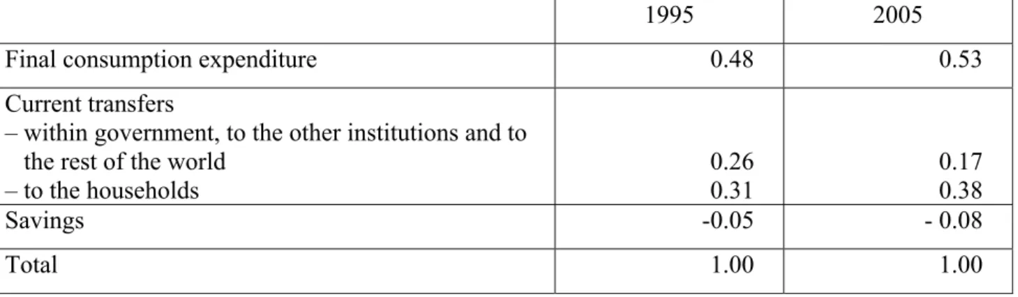
Table 12. Direct influences of unitary changes in the exogenous current receipts of the government
1995 2005
Final consumption expenditure 0.48 0.53
Current transfers
– within government, to the other institutions and to the rest of the world
– to the households 0.26 0.31 0.17 0.38
Savings -0.05 - 0.08
Total 1.00 1.00
Source: Tables A.1.1 and A.1.2
(columns dicg, corresponding to column 18, in both Table 4 and Table 5).
Note: Social transfers in kind represent a final consumption expenditure of the government and are not considered in the current transfers. In both years, social transfers in kind were about 60% of the government’s final consumption expenditure.
Accounting multipliers and their components, quantify a global influence on the endogenous accounts, which is quantified by the values of Tables 13 and 14, as follows.
Table 13. Global influences of unitary changes in the exogenous current receipts of the government
1995 2005
Aggregate Demand/Supply 0.968 0.831
Production Value/Total Costs 0.883 0.766
Aggregate Factors Income – Labour
– Own Assets 0.408 0.149 0.380 0.126
Aggregate Income – of the government
– of the other Institutions (except households) 1.317 0.097 1.187 0.064
Aggregate Investment/Investment Funds – of the government
– of the other Institutions (except households) - 0.101 0.026 - 0.123 0.004
Source: Tables A.1.3 and A.1.4
(columns dicg, corresponding to column 18, in both Table 4 and Table 5).
Apart from the effect on the aggregate income of the government, where 1 is the initial injection (leakage, in the case of scenario A) of income, the greatest effects of unitary changes in the current receipts of the government were felt on aggregate demand (supply) and production values (total costs), reflecting the great importance of final consumption for the total current outlays of the government, as noted earlier.
These global effects generally decreased from 1995 to 2005, meaning that the impacts of such a social policy measure on the whole economy were less noticeable in 2005.
Some more conclusions about these effects can be drawn from the multipliers’ components, as shown in Table 14.
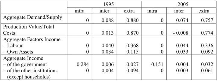
Table 14. Additional group influences of unitary changes in the exogenous current receipts of the government
1995 2005
intra inter extra intra inter extra
Aggregate Demand/Supply 0 0.088 0.880 0 0.074 0.757
Production Value/Total
Costs 0 0.013 0.870 0 - 0.008 0.774
Aggregate Factors Income – Labour
– Own Assets 0 0 0.040 0.034 0.368 0.115 0 0 0.044 0.033 0.336 0.092
Aggregate Income – of the government – of the other institutions (except households)
0.284
1995 2005
intra inter extra intra inter extra
Aggregate Investment/ /Investment Funds – of the government
– of the other institutions (except households)
0
0 - 0.001 0.023 - 0.100 0.003 0 0 - 0.001 0.015 - 0.122 - 0.011
Source: Tables A.1.5 – A.1.10
(columns dicg, corresponding to column 18, in both Table 4 and Table 5).
Thus, additional intragroup effects were felt only at the level of the aggregate income of the government. There is a clear predominance of additional extragroup influences, meaning that most of the repercussions originating from the current account of the government do not return to it, with the low values of the additional intergroup influences representing those repercussions that do in fact return.
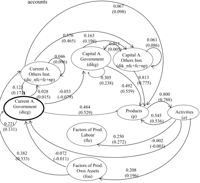
-0.053 (-0.079) 0.067 (0.098) 0.484 (0.529) 0.800 (0.788) 0.545 (0.536) 0.250 (0.272) -0.072 (-0.011) 0.221 (0.131) 0.208 (0.196) 0.382 (0.333) 0.028 (0.015) 0.123 (0.171) 0.046 (0.096) 0.576 (0.465) 0.492 (0.559) 0.813 (0.775) 0.013 (0.005) -0.002 (-0.003) 0.305 (0.238) 0.163
(0.198) 0.061
(0.086)
Figure 1. Scenario A - Network of elementary paths and adjacent circuits linking endogenous accounts
Note: This outline represents only the paths whose poles of origin and destination are the
endogenous accounts.
Source: Tables A.1.1 and A.1.2 (values in brackets)
Considering the importance of final consumption for the government, especially in the case of the products of group 6, relative to services16, which will be the social transfers in kind, the cells (p6, dicg) of the corresponding accounting multipliers (Tables A.1.3 and a.1.4) were decomposed through structural path analysis,in keeping with equation (20), with attention being
centred on the accounts of that group of products and of the government. Table 15 shows the results of this analysis.
16 Services other than wholesale and retail trade services, repair services, hotel and restaurant services, transport and communication services (products 4) and financial intermediation services, real estate, renting and business services (products 5). Capital A. Government (dikg) Current A. Government (dicg)
Factors of Prod. Labour
(fle)
Factors of Prod. Own Assets
(foa)
Products
Table 15. Structural path analysis of the global influences on aggregate demand of unitary changes in the exogenous current receipts of the government
1995 2005
Accounting Multiplier 0.659 0.642
Path 1 (dicg p6)
IT= ID* Mp 0.626 0.628
ID 0.459 0.498
Mp 1.363 1.260 Path 2 (dicg dikg p6)
IT= ID* Mp 0.000 0.000
ID 0.000 0.000
Mp 1.969 1.655 Other Paths (dicg … p6)
IT 0.033 0.014
Source: Tables A.1.3 and A.1.4.
Figure 1 helps us to see the linkages between accounts and how the impacts are widespread. Thus, path 1 directly links the current account of the government (dicg or 18) to the account of
the group of products 6 (p6 or 6) and absorbs almost all the impact, with the high values of the path multipliers showing that most of the impacts result from the adjacent feedback circuits. Path
2 makes the same link through the capital account of the government (dikg) and has no importance in terms of total influence, although its path multiplier has a higher value than in path 1, showing its important role in the amplification of the effects through the adjacent feedback
circuits. All the other paths have a significantly low importance.
The high values of the path multipliers help to underline the identified importance of the additional extragroup and intergroup influences, in the additional decomposition of the accounting multipliers.
It is important to remember that, with this methodology, apart from the unitary change in the current expenditures of households, through the reduction in the rate of direct taxes paid by households to the government (which is a direct effect), nothing more can be measured in terms of the global effects of that measure on the households’ aggregate income and aggregate investment/investment funds, since their current and capital accounts were set as exogenous.
d) Scenario B (increase in the social benefits other than social transfers in kind received by households from the government) – first results
Next, the effects or influences of unitary changes (an increase, in this case) in the households’ current income were identified, as follows.
Table 16. Direct influences of unitary changes in the exogenous current receipts of households
1995 2005
Final consumption expenditure 0.64 0.66
Current transfers
– within households, to the other institutions and to the rest of the world
– to the government 0.08 0.18 0.07 0.20
Savings 0.01 0.07
Total 1.00 1.00
Source: Tables A.1.11 and A.1.12
(columns dich, corresponding to column 15, in both Table 4 and Table 5).
In this scenario, Table 16 shows, through the average expenditure propensities, the direct influences of unitary changes in the exogenous current receipts of households – for instance in the social benefits paid by the government. Thus, more than a half (0.64 in 1995; 0.66 in 2005) of that unit is spent in final consumption and a significant part of the remainder represents current transfers to the government. Therefore, the direct effect of an increase in the current expenditures of the government, through an increase in the social benefits paid by the government to households, mainly means an increase in the final consumption expenditure and in the current receipts of households and, consequently, in the current receipts of the government (coming from households’ current transfers). Just as was seen in scenario A, this impact on the current receipts of the government cannot be measured using the multiplier methodology, since the accounts of the government are exogenous.
Tables 17 and 18 quantify and decompose the global influence of such changes on the endogenous accounts.
Table 17. Global influences of unitary changes in the exogenous current receipts of households
1995 2005
Aggregate Demand/Supply 2.897 2.467
Production Value/Total Costs 2.294 1.926
Aggregate Factors Income – Labour
– Own Assets 0.512 0.492 0.472 0.403
Aggregate Income – of the households
1995 2005 Aggregate Investment/Investment Funds
– of the households
– of the other institutions (except government) 0.212 0.185 0.139 0.132
Source: Tables A.1.13 and A.1.14
(columns dich, corresponding to column 15, in both Table 4 and Table 5).
In this case, apart from the effect on the aggregate income of households, where 1 is the initial injection of income, the greatest effects (of unitary changes in the current receipts of households) were felt in a similar way to scenario A, but now more than twice as intensely at the level of the aggregate demand (supply) and production values (total costs), reflecting the great importance of final consumption for the total current outlays of the households, as seen in Table 13.
In this scenario, a general decrease in the global effects can also be noted from 1995 to 2005. This is shown in Table 18, where, at all levels of impact, the additional extragroup influences are dominant; the intergroup effects are almost insignificant and the intragroup effects almost null. Therefore, as was seen in scenario A, most of the repercussions originating from the current account of households do not return to it.
Table 18. Additional group influences of unitary changes in the exogenous current receipts of households
1995 2005
intra inter extra intra inter extra
Aggregate Demand/Supply 0 0.462 2.435 0 0.387 2.079
Production Value/Total Costs 0 0.321 1.973 0 0.248 1.678
Aggregate Factors Income – Labour
– Own Assets 0 0 0.090 0.093 0.423 0.398 0 0 0.080 0.078 0.392 0.325
Aggregate Income – of the households – of the other institutions (except government)
0.006
0 0.164 0.053 0.705 0.243 0.006 0 0.128 0.039 0.592 0.194
Aggregate Investment/ /Investment Funds – of the households
– of the other institutions (except government)
0
0 0.031 0.045 0.181 0.140 0 0 0.020 0.031 0.119 0.101
Source: Tables A.1.15-A.1.20
(columns dich, corresponding to column 15, in both Table 4 and Table 5)
Structural path analysis helps us to understand these effects, through the schematic
0.104 (0.069) 0.067 (0.098) 0.636 (0.662) 0.800 (0.788) 0.545 (0.536) 0.250 (0.272) 0.595 (0.502) 0.998 (0.995) 0.006 (0.006) 0.208 (0.196) 0.382 (0.333) 0.050 (0.044) 0.179 (0.171) 0.046 (0.096) 0.576 (0.465) 1.130 (1.171) 0.813 (0.775) 0.061 (0.072)
Figure 2. Scenario B - Network of elementary paths and adjacent circuits linking endogenous accounts
Note: This outline represents only the paths whose poles of origin and destination are the
endogenous accounts.
Source: Tables A.1.13. and A.1.14. (values in brackets)
Table 16 shows that the direct influences of unitary changes in the exogenous current receipts of households were centred mainly on their final consumption, thus underlining the importance of group 2, relating to manufactured products and energy products (as well as products from mining and quarrying). The cells (dich, p2) of the corresponding accounting multipliers were decomposed through structural path analysis, in keeping with equation (20), paying special
attention to the accounts of that group of products and of households. The results are shown in Table 19. Capital A. Households (dikh) Current A. Households (dich)
Factors of Prod. Labour
(fle)
Factors of Prod. Own Assets
(foa)
Products
Table 19. Structural path analysis of the global influences on aggregate demand of unitary changes in the exogenous current receipts of households
1995 2005
Accounting Multiplier 1.521 1.187
Path 1 (dich p2)
IT= ID* Mp 1.086 0.894
ID 0.366 0.342
Mp 2.967 2.611 Path 2 (dich dikh p2)
IT= ID* Mp 0.047 0.020
ID 0.016 0.008
Mp 2.978 2.624 Other Paths (dich … p2)
IT 0.388 0.273
Source: Tables A.1.13 and A.1.14.
The studied paths can be identified in Figure 2, in which the other linkages between endogenous
accounts can also be identified. Almost all of the global influence is centred on path 1, which
directly links the current account of the households (dich) to the account of products 2 (p2); path 2, which makes the same link through the capital account of the households, has an almost
insignificant (global) influence, especially if compared with the other paths. Mention should be
made here of the values of the path multipliers, which, besides confirming the already identified
importance of the additional extragroup and intergroup influences in the additional decomposition of the accounting multipliers, show the important role played by those paths in the amplification of these effects through the adjacent feedback circuits.
As in scenario A, it is important to bear in mind that, with this methodology, apart from the unitary change in the current expenditures of the government, through the increase in the social benefits paid by the government to households (which is a direct effect), nothing more can be measured in terms of the global effects of that measure on the government’s aggregate income and aggregate investment/investment funds, since their current and capital accounts were set as exogenous.
3.2. The SAM-based linear model
As can be confirmed by comparing the structure of this model with the structure of the underlying database, or numerical version, presented in section 2, all the transactions of the national accounts are identified, although a significant part are still considered as exogenous. Parameters were calculated from the data used for the construction of the numerical versions, from which the exogenous variables were also identified.
The GAMS (General Algebraic Modelling System) software was used to run this model – firstly to calibrate it and then to perform the experiments associated with the described scenarios.
In this version of the model, it will be assumed that all domestically produced output is market output, and therefore any output produced for own final use and other non-market output will be considered as non-existent – the author hopes that this assumption can be eliminated in a future version of this model. On the other hand, since there is sufficient production capability available in the economy and imports are exogenous, domestic output will respond exclusively to aggregate demand.
Table 20. The formalized transactions (cells) in the basic SAM
p a f dic dik dif rw total
p – products tp p tp a 0 tp dic tp dik 0 tp rw tp.
a – activities ta p 0 0 0 0 0 0 ta .
f – factors of production 0 tf a 0 0 0 0 tf rw tf .
dic – current account of the (domestic)
institutions tdic p tdic a tdic f tdic dic 0 0 tdic rw tdic .
dik – capital account of the (domestic)
institutions 0 0 0 tdik dic tdik dik tdik dif tdik rw tdik .
dif – financial account of the (domestic)
institutions 0 0 0 0 0 tdif dif tdif rw tdif .
rw – rest of the world trw p trw a trw f trw dic trw di k trw dif trw.
total t.p t.a t.f t.dic t.dik t.dif t.rw
cell Equations (or exogenous variables)
See “conventions and declarations” in the Appendix (A.2.3.) Eq.nº
Compensation of factors of production
tf a Gross Added Value
GAVf,a = dbsf,a*GAVa (22)
GAVa = βa*VPa (23)
GAVf = ΣaGAVf,a (24)
tf rw Compensation of Factors(Received) from the rest of the world
CFRf,rw ---
tdic f Gross National Income
cell Equations (or exogenous variables)
See “conventions and declarations” in the Appendix (A.2.3.) Eq.nº
GNIf = GAVf+CFRf,rw-CFSrw,f (26)
GNIdic = ΣfGNIdic,f (27)
GNI = ΣdicGNIdic (28)
trw f Compensation of Factors (Sent) to the rest of the world
CFSrw,f ---
Production
ta p VPp = ADp-TMTp-NTPp-IMp (29)
VPa,p = VPp*αa,p (30)
VPa =ΣpVPa,p (31)
External Trade
tp rw Exports
EXp,rw ---
trw p
(part) IIMmportsrw,p ---
Net indirect taxes or net taxes on production and imports
Net Taxes on Production (of Activities)
tdic a NTAdic,a= ntagdic,a*NTAAa (32)
NTAdic= ΣaNTAdic,a (33)
NTAa= ΣdicNTAdic,a (34)
trw a NTArw,a= ntarwrw,a*NTAAa (35)
NTArw= ΣaNTArw,a (36)
NTA = ΣdicNTAdic+NTArw (37)
Net Taxes on Products
tdic p NTPdic,p= ntpgdic,p*NTPp (38)
NTPdic= ΣpNTPdic,p (39)
trw p
(part) NTPrw,p= ntprwrw,p*NTPp (40)
NTPrw = ΣpNTPrw,p (41)
NTPp = tpp*DTp (42)
NTP = ΣdicNTPdic +NTPrw (43)
Trade and Transport Margins
tp p TMp,p = tmrp,p*DTp (44)
TMPp = p TMp,p(column sum) (45)
Domestic Trade
DTmpp = VICp + FCp + GCFp (46)
DTp = DTmpp - TMPp - NTPp (47)