Semiclassical limit of the EPRL spin foam model

(1)

UNIVERSIDADE DE LISBOA FACULDADE DE CIÊNCIAS DEPARTAMENTO DE FÍSICA

Semiclassical Limit of The EPRL Spin Foam Model

Miguel João de Lopes Marques

Mestrado em Física

Especialização em Astrofísica e Cosmologia

Versão Provisória

Dissertação orientada por:

Prof. Doutor Aleksandar Miković

Prof. Doutor José Pedro Oliveira Mimoso

(2)

(3)

Acknowledgements

I would like to thank my supervisor, professor Aleksandar Miković, for his precious help, my girlfriend Margarida Mendes, for always believing in me, my friend André Silva for all the jokes provided, and to all my friends and family, for their tremendous support.

(4)

(5)

Abstract

One of the pressing issues of present-day theoretical physics is the need for the quantisation of gravity. Although Einstein’s theory of general relativity (GR) has experienced tremendous success as a classical theory of gravity, it faces a number of problems, including the existence of singularities in high-curvature regimes, such as the centre of a black hole or the Big Bang. In such scenarios, quantum effects of the geometry of spacetime are posited to play an important role, thus begging the formulation of a theory of quantum gravity. Such an endeavour naturally leads to several different approaches, which generally take the main assumptions from either quantum field theory or general relativity and attempt to account for the other a posteriori.

In this dissertation, we opt for the use of general relativity as a starting point for quantising gravity and present the background independent non-perturbative canonical quantisation approach known as “loop quantum gravity”. From this theory, it is possible to construct objects known as “spin foams”, which allow us to explore its dynamics from a covariant perspective. More specifically, the spin foam quantization of general relativity is a path integral quantization based on the loop quantum gravity approach, where the gravitational field is described by “spin networks”. These spin networks can be understood as Wilson loop variables for the Ashtekar formulation of GR. Within the Engle-Pereira-Rovelli-Livine (EPRL) spin foam model, the transition amplitudes are constructed by using the topological gravity theory based on the BF theory for the Lorentz group and the constraints which define GR are then imposed on them.

Consistency of any quantum gravity theory requires its correspondence to general relativity in the low-energy scale and this prompts us to analyse the semiclassical limit of the aforementioned EPRL model. The study of such a limit is performed through the use of the effective action approach from background field method of quantum field theory, which yields a generalisation of GR — in the sense that it allows non-metric geometries — as the semiclassical limit of the EPRL model. In other words, the leading term of the one-loop effective action of the EPRL model corresponds to the area-Regge action, which is based on the Regge action discretising gravity.

Finally, after presenting the review described above, we discuss a version of Regge calculus which takes triangle areas and 3d angles as variables, define a new convergent state sum from it and extend the theory in order to include a particular type of Lorentzian triangulation.

(6)

(7)

Resumo

A teoria da relatividade geral de Einstein é a teoria gravitacional mais bem-sucedida. No entanto, é também uma teoria incompleta, uma vez que contém regimes em que diverge para o infinito e se torna incapaz de efectuar qualquer previsão. Tais regimes são referidos como “singularidades” e ocorrem em cenários de alta curvatura, tal como no centro de buracos negros e no “Big Bang”. Assim sendo, é necessário modificar esta teoria de forma a evitar singularidades. A principal solução proposta na lit-eratura é a quantização da gravidade, uma vez que se supõe que no contexto referido as fluctuações quânticas da geometria desempenhem um papel importante na acção gravítica. Esta solução provém de uma longa história de quantizações de teorias clássicas que continham divergências ultravioletas. À semelhança de tais teorias — como por exemplo o modelo do átomo de hidrogénio —, espera-se que os problemas enfrentados pela relatividade geral sejam eliminados. Por outro lado, uma teoria de gravitação quântica aproximar-nos-ia de uma unificação das quatro forças fundamentais numa só “teoria de tudo”.

Relativamente à unificação da mecânica quântica com a relatividade geral, existem duas aborda-gens principais: a primeira adopta os pressupostos da mecânica quântica e tenta incluir a relatividade geral a posteriori, enquanto que a segunda faz o inverso. As teorias mais bem-sucedidas dentro de cada abordagem são, respectivamente, a teoria de cordas e a teoria de gravidade quântica em laços. Nesta dissertação defendemos a segunda, dada a sua natureza independente do fundo — isto é, independente da escolha de uma métrica de fundo — e não-perturbativa. De facto, é argumentado que, num regime de alta curvatura, o método perturbativo não é aconselhável, uma vez que existem várias possibilidades de escolha para o par fundo-perturbação da métrica, o que leva ao surgimento de múltiplos cones de luz, que por sua vez levam a relações de causalidade distintas e incompatíveis.

A teoria de gravidade quântica em laços é uma teoria quântica da geometria do espaço-tempo que con-siste na quantização canónica (ou Hamiltoniana) da relatividade geral, originando uma teoria de gauge

SU (2), semelhante à de Yang-Mills. Contudo, embora a gravidade quântica em laços tenha tido muito

sucesso — como por exemplo a concordância com a relatividade geral no limite clássico — e faça pre-visões únicas — como a discretização do espaço-tempo à escala de Planck e a possível resolução de singularidades, como por exemplo a substituição do “Big Bang” pelo “Big Bounce” —, a mesma sofre de alguns problemas, como a definição da dinâmica quântica no contexto referido.

A solução estudada para o problema da dinâmica envolve o uso de espumas de spin, que podem ser vistas como uma formulação de integral de caminho da gravidade quântica em laços. As espumas de spin são também uma “história quântica” das redes de spin, que por sua vez são as configurações permitidas para as excitações do campo. Em geral, os modelos de espumas de spin para a relatividade geral em quatro dimensões começam por discretizar a relatividade geral, depois quantizam a parte BF topológica da nova teoria discreta e finalmente impõem os constrangimentos simpliciais ao nível quântico. No caso do conhecido modelo Barrett-Crane, a quantização é efectuada na acção SO(4) simplicial de Plebanski. Contudo, os constrangimentos de Plebanski — que reduzem a teoria de BF à relatividade geral — são impostos fortemente, o que leva a condições adicionais desnecessárias.

O modelo EPRL, por sua vez, é uma modificação do modelo Barrett-Crane, que discretiza a relativi-dade geral, quantiza a mesma e finalmente impõe e relaxa os constrangimentos de Plebanski. Este último passo diferencia este modelo do anterior e resolve muitos dos problemas enfrentados pelo mesmo. Em relação ao primeiro passo, a discretização é feita recorrendo ao uso de uma triangulação em 4d que é dual ao complexo representado pela espuma de spin e onde spins inteiros são atribuídos a faces e um elemento

(8)

da base do espaço de “intertwiners” a cada aresta. Consequentemente, obtemos o espaço de redes de spin da gravidade quântica em laços SO(3) Hamiltoniana como espaço de estados da teoria, assim como uma amplitude de vértice covariante sob SO(3) e SO(4).

Uma vez que a consistência de qualquer modelo de gravidade quântica está intimamente ligada à convergência da mesma para a relatividade geral, no limite clássico, é importante certificarmo-nos de que o modelo EPRL se reduz à (ou converge para a) teoria de Einstein no limite de baixas energias. Para o efeito, usamos o método da acção efectiva, proveniente do método de campo de fundo da teoria quântica de campo. Este método consiste em aplicar a fórmula da acção efectiva aos modelos de espuma de spin e somar as fluctuações em volta de uma configuração clássica. A acção efectiva permite-nos obter o limite semiclássico de qualquer modelo de espuma de spin e pode ser aplicada a qualquer modelo de soma de estados de gravidade quântica. No caso do modelo de EPRL, é necessário modificar a amplitude do vértice de forma a obter o limite semiclássico correcto, ou seja, uma generalização da teoria da relatividade geral — no sentido em que permite geometrias não-métricas. A modificação necessária envolve a divisão da amplitude (mencionada acima) pelo produto de uma função homogénea de ordem 12 do spin e da soma das dimensões do spin elevadas a um número positivo e suficientemente grande. Desta forma, a soma de estados do modelo torna-se finita e converge para o limite supramencionado, ou seja, a acção área-Regge. Por outras palavras, o primeiro termo da accção efectiva de primeira ordem emℏ do modelo EPRL corresponde à acção área-Regge, baseada na acção Regge, que, por sua vez, discretiza a relatividade geral de Einstein. A acção área-Regge difere, contudo, da primeira, uma vez que usa as áreas das faces como variáveis, ao invés dos comprimentos das arestas, como na acção Regge.

Após o cálculo do limite semiclássico do modelo EPRL, apresentamos uma versão modificada do cálculo Regge, uma vez que este último é incapaz de definir uma medida invariante de gauge na integral de caminho. Esta teoria usa áreas de triângulos — seguindo os passos da teoria topológica BF —, assim como ângulos em 3d, que constrangem as áreas. O resultado é uma acção que impõe dois conjuntos de constrangimentos sobre a acção (comprimento-)Regge: o primeiro exige que a definição dos ângulos 2d em termos de ângulos 3d seja a mesma, independentemente do tetraedro escolhido (dos 2 possíveis para o primeiro ângulo), enquanto que o segundo inclui as áreas dos triângulos na definição da condição de fecho dos tetraedros. O efeito dos constrangimentos é a redução da acção área-ângulo Regge para a acção comprimento Regge.

Finalmente, é apresentada uma modificação da acção área-ângulo Regge que inclui triangulações Lorentzianas. Estas triangulações consistem na foliação do espaço tempo em camadas com 3 dimensões, representando cada uma um tempo discreto. Estas camadas possuem símplices espaciais de dimensão 3 e estão interligadas por arestas temporais, formando assim símplices temporais de dimensão 4. Os comprimentos das arestas espaciais são fixos e iguais para todas as arestas desse tipo e o mesmo acontece para as arestas temporais (com um comprimento diferente das anteriores). Obtendo a fórmula que nos dá os ângulos 2d em termos dos ângulos 3d para este tipo de símplices Lorentzianas permite-nos modificar os constrangimentos anteriores de forma a acomodar os casos Euclideano e Lorentziano.

A criação de um modelo de soma de estados para esta nova acção, assim como a modificação ade-quada desse modelo (por forma a garantir a sua convergência), a aplicação do método da acção efectiva ao mesmo e a generalização da nova acção para outros casos Lorentzianos são deixados para um trabalho futuro.

Palavras-Chave: espuma de spin, limite semiclássico, modelo EPRL, acção efectiva, cálculo de

Regge

(9)

List of Figures

1.2.1 Light cone derived from the choice of a background metric ηaband (smaller) light cones resulting from the quantum perturbations added to said metric. It is an inconsistent rep-resentation of the gravitational field, since the field excitations are expected to obey the main light cone, which itself bears no meaning in the context of GR, a theory which does not admit any preferential reference frame or background [1]. . . 3 2.2.1 A spin network state where the vertices are connecting 3 edges (i.e. they are 3-valent).

In this case, the contraction in the central vertex ψ is unique and given by a Clebsh-Gordan coefficient (or intertwiner), unlike for higher valence vertices, where a choice of a higher-order tensor from several coefficients is necessary [2]. . . 8 2.2.2 A 4-valent vertex can be defined as two 3-valent ones and other assignments of pairs of

edges (e.g. 1-3, 2-4) are equally possible, provided we use the correct intertwiners in the wave function equation [2]. . . 9 3.1.1 A spin foam describing the transitions between 3 different spin networks, forming a

2-complex (left), and a transition vertex (right) within the spin foam. The transitions be-tween spin networks occur from bottom to top and, as one can easily notice, with each transition, new links are created and the spins are reassigned at the vertices [3]. . . 12 6.2.1 Possible simplices in 2 (top), 3 (middle) and 4 (bottom) dimensions, (up to time reversal

for 3 and 4 dimensions): (2, 1)- and (1, 2)-simplices (top left) and the resulting gluing (top right); (3, (middle left) and (2, 2)- (middle right) tetrahedra/simplices; (4, 1)-(bottom left) and (3, 2)- 1)-(bottom right) simplices. The 2-dimensional strip (top right) is eventually joined at both ends, forming a band with topology S1× [0, 1] [4]. . . 43

(12)

(13)

List of Tables

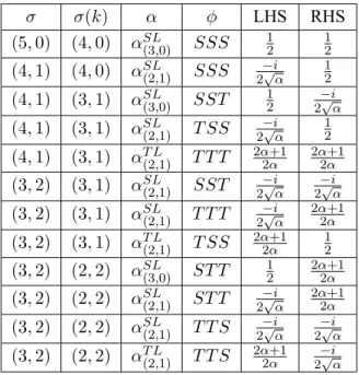
B.1 Possible left- (LHS) and right-hand side (RHS) combinations (up to the commutation of the second and third terms in ϕ) for the equation 6.1.1, along with their geometric interpretation: the 4-simplex σ; the resulting tetrahedron σ(k); the 2d angle α appearing on the left-hand side; and the 3d angle ϕ combinations. The notation used has been explained earlier. . . 71

(14)

(15)

List of Abbreviations

BC Barrett-Crane

CERN European Organisation for Nuclear Research EPRL Engle-Pereira-Rovelli-Livine

FK Freidel-Krasnov GR General Relativity LQG Loop Quantum Gravity QFT Quantum Field Theory

(16)

(17)

Chapter 1

Introduction

1.1 Gravity

One of the staples of scientific theories is the fact that they are not immutable. In addition, the strength of a theory is highly dependent on the number of accurate predictions it makes. This means that any unaccounted phenomenon is enough to warrant a modification of the underlying theory, or even the de-velopment of a new one. This has often been the case throughout scientific history, including the history of gravitational physics.

Up until the last century, the reigning theory of gravity was Newton’s law of universal gravitation, which treated it as a force between any two particles, which was proportional to the product of their masses and inversely proportional to the square of the distance between them. This theory boasted a number of important achievements, the most important of which was arguably the prediction of the existence of a planet beyond Uranus — later discovered and named Neptune —, which was influencing its orbit.

However, some conflicting observations were later made, including the discrepancy between the precession of the perihelion of Mercury’s orbit and the respective Newtonian calculations. Initial attempts to explain this discrepancy by means of a new planet between Mercury and the Sun were unsuccessful and thus the road was paved for a new theory of gravity.

Such a theory came about in the beginning of the 20thcentury, through Albert Einstein. This time, gravity was considered a geometric property of space and time — henceforth named spacetime — and a connection was established between the spacetime curvature and the energy and momentum of matter (and radiation) within it. In a nutshell, it can be summarised by the following quote, by John Archibald Wheeler: “Spacetime tells matter how to move; matter tells spacetime how to curve”. General relativity was a tremendous achievement: not only was it able to solve the problems plaguing Newton’s theory — such as the aforementioned precession of Mercury — but it also introduced new important concepts and predictions, such as gravitational time dilation, lensing and redshift, as well as black holes and gravita-tional waves, all of which have been confirmed by numerous observations.

Einstein’s theory of general relativity is currently the most complete, accurate and widely accepted description of gravity. However, despite the overwhelming evidence in its favour, there are a number of unsolved problems which render this theory incomplete, including the existence of spacetime singulari-ties. These singularities occur in spacetime locations where the gravitational field of an object, its energy density and the spacetime curvature around it — which are related to one another via the Einstein field equations (EFE) — all become infinite. In such a scenario, as is the case for the centre of a black hole , as well as the Big Bang, the laws of physics break down and general relativity is unable to provide any prediction.

(18)

The problems faced by general relativity suggest that this theory of gravity is incomplete and thus should be modified, by analogy with the case of Newton’s theory. More closely related to these issues, however, are the ultraviolet catastrophe of blackbody radiation and the classical model of the hydro-gen atom. Both of these models are classical and entail singularities which are avoided by taking the appropriate quantum effects into account, at small (distance) scales [1].

These examples are taken as a sign that Einstein’s theory should be modified so as to include quan-tum degrees of freedom. In fact, while general relativity has succeeded in describing the universe at cosmological scales, quantum mechanics has experienced the same for subatomic scales. It is therefore paramount to conciliate these two theories, since doing so would be a step further in formulating a “theory of everything”, i.e. a theory encompassing all four fundamental forces under the same framework.

1.2 Quantum Gravity

As mentioned above, both general relativity and quantum mechanics benefit from a significant amount of experimental evidence. Nonetheless, the unification of both theories is not straightforward, meaning at least one of them requires some level of modification. Consequently, one must choose which aspects of each theory are assumed to be correct and will therefore be used as a starting point for the development of an all-encompassing framework [5].

At first glance, the most sensible approach might seem to be the quantum field theory (QFT) formal-ism, since it has been successfully used as a description of the other three fundamental forces. Neverthe-less, even though QFT can be used as an effective field theory for gravity at low energies, this method is troublesome when applied to high energies, due to the fact that general relativity is nonrenormalisable in such scales.

Renormalisation techniques are essential in ridding quantum field theories of undesirable divergences, by introducing “counterterms” which end up cancelling them. However, when the required number of counterterms becomes infinite, so does the number of free parameters, thereby stripping the theory of any predictive power. In this kind of scenario, said theory is defined as “nonrenormalisable” and that is precisely the case with Einstein’s theory [1].

One way of overcoming these difficulties is to substitute the concept of a point-like particle for a string-like — i.e. one-dimensional — one. This gives rise to “string theory”, or “superstring theory”, in its latest form. Despite being a mathematically elegant solution to the problem of unifying gravity and quantum mechanics and being a very prolific research area, superstring theory possesses significant shortcomings, the main one being the number of unverified assumptions that are made. In a daring challenge to Occam’s razor, this approach relies on the existence of several extra dimensions of space, as well as new particles, all of which is yet to be observed at CERN, despite extensive experiments.

As a result, there is good reason to accept the main premisses of general relativity and build a new theory from there, in lieu of quantum mechanics, quantum field theory or particle physics. One of the fun-damental aspects of general relativity is the fact that it satisfies the principle of general covariance, which implies that the laws encompassed by this theory are the same for any coordinate system or reference frame, thus being invariant under coordinate transformations and remaining unchanged for any observer. In addition, it is also a background independent theory, since the gravitational field is not attached to any fixed background structure.

Considering general relativity as the best description of gravity thus far [6], it is reasonable to borrow its aforementioned features — i.e. general covariance and background independence — for a quantum gravity theory [6]. In light of that, we can point further obstacles to using quantum field theory within this

(19)

Figure 1.2.1: Light cone derived from the choice of a background metric ηaband (smaller) light cones resulting from the quantum perturbations added to said metric. It is an inconsistent representation of the gravitational field, since the field excitations are expected to obey the main light cone, which itself bears no meaning in the context of GR, a theory which does not admit any preferential reference frame or background [1].

scenario. Firstly, QFTs are only defined for a fixed spacetime (background) geometry and are thus not generally covariant. Additionally, even though the ultraviolet divergences — i.e. high energy singularities — in these theories should in principle vanish upon accounting for quantum spacetime fluctuations, that can only be done by taking the dynamics of spacetime into account, which, by definition, forbids the use of fixed backgrounds [1].

An area closely related to background dependence is perturbation theory. Due to the relation between these two concepts, as well as the aforementioned problems with the former in the gravitational frame-work, a non-perturbative theory of gravity is generally considered to be the best approach when it comes to defining a quantum gravity theory. In order to understand the reasoning leading to this statement, we must first present the consequences of a perturbative approach to quantum gravity [1].

Perturbation theory is a method whereby a complex (quantum) system is described as the result of small perturbations to a simpler system, to which we know the solution. In the context of quantum gravity, this simpler system is regarded as a fixed background metric ηab, on top of which we add metric fluctuations, hab. The resulting metric tensor is then

gab= ηab+ hab, (1.2.1)

and this is appropriately applied to nearly-flat spacetime. However, in a high-curvature setting, such as the one where the study of quantum gravity is applied, the same spacetime metric can be equivalently represented by other background-perturbation pairs, meaning we can also have

gab= η′ab+ h′ab, (1.2.2)

where η_ab′ ̸= ηab. This new background metric can represent a different light cone and thus lead to different causality relations from the original one. Since the background spacetime is what allows one to define causality relations in perturbation theory, it is contradictory to choose a background (and thus a causal structure or light cone) with no a priori physical meaning to which the gravitational field has to adhere, when in reality the quantum excitations of this field can generate different light cones. In other words, the mandatory background imposed by perturbation theory not only clashes with the covariant and background independent nature of general relativity, but is also devoid of any physical importance, when compared to other possible “backgrounds” (e.g. η′_ab) — as shown in Figure 1.2.1 [1].

(20)

The ambiguities presented above show that a standard perturbative approach to a covariant system is not a consistent one and thus the most logical path involves defining a non-perturbative theory of quantum gravity. Thus, to summarise the main ideas discussed in the last two chapters: it is crucial to formulate a theory of quantum gravity which is not only consistent with general relativity (by identifying it as its clas-sical limit) [1] but also able to consistently describe the physics of singularities by taking quantum effects into account, at small scales. In order to accomplish the former goal, the resulting quantum gravity theory must obey the same principles as Einstein’s, namely general covariance and background independence, as well as being non-perturbative. One such theory is named loop quantum gravity [6].

(21)

Chapter 2

Loop Quantum Gravity

2.1 Overview

Loop quantum gravity is an attempt to perform a mathematically sound background independent and non-perturbative quantisation of general relativity. Following the idea from general relativity that gravity is spacetime geometry, loop quantum gravity becomes a theory of quantum geometry that is diffeomorphism invariant, i.e. it is invariant under isomorphisms to other smooth manifolds [1].

The loop quantum gravity approach [7, 8] consists of using the canonical (i.e. Hamiltonian) quanti-sation of general relativity via connection variables. General relativity is then transformed into an SU (2) gauge theory, similar to the Yang-Mills theory. However, even though this theory boasts many achieve-ments — such as the consistency with general relativity in the classical limit — and makes unique pre-dictions — such as the discretisation of space at the Planck scale —, it has also encountered obstacles, such as the problem of defining quantum dynamics within such a framework. Fortunately, this particular problem might be solved with the use of spin foams, which will be presented later in this chapter [1]. For now, we will describe how loop quantisation is performed [6].

As mentioned above, the Hamiltonian formulation of general relativity is the starting point for loop quantum gravity [6, 9]. In this formulation, we foliate the usual 4d spacetime into a series of spatial slices Σ evolving in time, with a 3-metric qab induced on them. In order to relate coordinates between different spatial slices, we use two Lagrange multipliers: the lapse function N and the shift vector Na (where a is a spatial index). While the former measures the proper time, the latter measures changes in the spatial coordinates. These two multipliers impose the constraints which imbue general covariance in GR: the scalar/Hamiltonian constraint and the diffeomorphism/vector constraints. Thus, the information is embedded in the spatial metric qab, as well as in the extrinsic curvature Kab.

In formulating GR as a gauge theory, LQG follows the Ashtekar-Barbero formalism [6, 10], which uses an SU (2) gauge connection, called the Ashtekar-Barbero connection, Ai_a, and densitised triad, E_ia (where both indices i are SU (2)) as canonical coordinates. In fact, one easily notices that the latter is the canonically conjugate momentum of the former. We define the aforementioned 3-metric using two other important elements, called the triad, ea

i, and its inverse, the co-triad, eia. The relations are then qab= eiae

j

bδij; (2.1.1)

and

(22)

while the densitised triad mentioned earlier is defined as

E_ia=√qea_i. (2.1.3)

To complete the canonical pair (A, E), we need only define the Ashtekar-Barbero connection:

Ai_a= Γi_a+ γK_ai, (2.1.4)

where K_ai = Kabebjδijis the extrinsic curvature and Γiais the spin connection consistent with Eia. Finally, we have the Poisson bracket

{

Aa_i(x), E_bj(y) }

= 8πGγδa_bδ_ijδ(x− y), (2.1.5) where γ is the Immirzi parameter, which measures the size of the quantum of area in Planck units. Disre-garding matter for now, we can express the constraints mentioned earlier, as well as a new one, in terms of the new variables (A, E):

• Gi = ∂aEia+ ϵijkΓjaEak = 0 is the new Gauss/gauge constraint, introduced due to the invariance of the Euclidean metric under SU (2) rotations;

• Ca= F_abi Eib= 0 is the diffeomorphism/vector constraint; • C = √ 1

|det(E)|ϵijk [

F_abi − (1 + γ2)ϵi_mnK_amK_bn]EajEbk= 0 is the scalar/Hamiltonian constraint, where Fi

abis the curvature tensor of the connection A.

In the loop quantisation, the phase space is described by holonomies and fluxes [6], which are later transformed into quantum variables. The advantages of using these variables are threefold: they are diffeomorphism invariant, as required by the main goal of LQG; the holonomies behave well under gauge transformations; and the Poisson bracket of these variables is well-defined. Put simply, the holonomy of a connection is a mathematical concept used for determining how much a parallel transport around a closed loop fails to preserve the transported information. For a connection A, its holonomy along an edge e is he(A) = P e ∫ edx a_Ai a(x)τi_. _(2.1.6)

In the equation above, P is the path ordering and τiare the SU (2) generators. The conjugate momentum of the holonomy is the flux of the densitised triad — which in LQG plays the role of an electric field — over surfaces S, defined as

E(S, f ) =

∫ S

fiE_iaϵabcdxbdxc, (2.1.7) where fi is an SU (2)-valued function used to smear the flux [6]. Finally, the Poisson bracket of these two variables is given by

{E(S, f), he(A)} = 2πGγϵ(e, S)fiτihe(A), (2.1.8) where ϵ(e, S) = 0 if e and S do not intersect one another or if e⊂ S. If e and S intersect at one point, we get ϵ(e, S) =±1, depending on their relative orientation.

The so-called holonmy-flux algebra presented here is associated to a kinematical Hilbert space, de-fined as the completion of the space of cylindrical functions, with respect to the Ashtekar-Lewandowski

(23)

measure [6]. We define a generalised connection ¯Aeas a map from an analytic path within a spatial slice to SU (2), while a collection of such paths intersecting at most at their ends is called a graph. For a closed graph Γ with n edges, a cylindrical function with respect to said graph is written as

ψΓ( ¯A) = fΓ( ¯Ae1, ..., ¯Aen), (2.1.9)

where ¯A is an element of SU (2), fΓis a function on SU (2)nand e is a path on a spatial slice. We also

define

Cyl =∪

Γ

CylΓ (2.1.10)

as the space of all cylindrical functions with respect to any graph in a spatial sector. Furthermore, we can use the Ashtekar-Lewandowski measure to obtain the inner product on this space:

⟨ ψΓ, ψ ′ Γ ⟩ = ∫ SU (2)n ∏ e⊂Ξ ΓΓ′ dheψ¯Γψ ′ Γ, (2.1.11)

where Ξ is a graph such that Γ, Γ′ ⊂ Ξ_ΓΓ′, Γ′ is the graph with respect to which ψ_Γ′ is cylindrical and

dh is the normalised Haar measure on SU (2). We can now define the kinematical Hilbert space as the

Cauchy completion of the space of all cylindrical functions in the Ashtekar-Lewandoswki norm. The basis of this space is composed of so-called spin network states, which are cylindrical functions with respect to a graph where each edge is coloured using an irreducible (and non-trivial) representation of SU (2). Naturally, by definition of basis, we know that any cylindrical function can be expanded in these states. We will delve into these spin network states later on.

We can now define the quantum operators for the flux and the holonomies. The former is given by ˆ EΓ(S, f ) = i2πGℏ ∑ e⊂Γ ϵ(e, S)T r ( fiτiA¯e ∂ ∂ ¯Ae ) , (2.1.12)

while the latter acts by multiplication [6]. In defining any general quantum operator, we must perform regularisation, which comprises the following steps:

1. The spatial manifold is triangulated into tetrahedra;

2. We use the Riemann sum over these cells, instead of the usual integral over the manifold;

3. We assign a regularised expression (in terms of the basic operators) to each cell, which must con-verge to the classical one when the cell vanishes;

4. If the expression is densely defined on the kinematical Hilbert space, it can be written as a quantum operator, independently of the regularisation.

As mentioned earlier, one of the most important consequences of this procedure is the discretisation of the spectra of such geometrical operators as area and volume, which thus give us an equally discrete manifold, at the Planck scale. This unique result is extremely useful when bypassing the singularities of general relativity.

The remaining step is to solve the quantum constraints, i.e. the Gauss, the diffeomorphism and the Hamiltonian constraints. Although the first two are solvable, finding the solution to the last one is a complicated task, as there are ambiguities when quantising the corresponding operator.

(24)

Figure 2.2.1: A spin network state where the vertices are connecting 3 edges (i.e. they are 3-valent). In this case, the contraction in the central vertex ψ is unique and given by a Clebsh-Gordan coefficient (or intertwiner), unlike for higher valence vertices, where a choice of a higher-order tensor from several coefficients is necessary [2].

After having defined the loop quantisation of gravity, we are left with the task of studying the dy-namics of such a system and this is where the spin foam approach is used. However, before introducing the concept of spin foam, it is imperative to first discuss spin networks, as the former can be seen as the evolution (or quantum history) of the latter.

2.2 Spin Networks

In loop quantum gravity, the space of spin networks corresponds to the initial kinematical Hilbert space and the goal is to reduce it to a physical one, where all the constraints are satisfied. While the solution to the Gauss constraint lies within the former, the same does not hold for the diffeomorphism ones, which forces us to define the latter (larger) space [2].

LQG posits that the Planck-scale geometry is foam-like and that the field excitations only occur on specific configurations of edges connected by vertices, called spin networks [2]. These networks are graphs Γ which are discrete, finite and embedded in the (continuous) spatial manifold Σ. The edges

ei ∈ Γ are connected at the vertices v ∈ Γ and each one has a holonomy he[A] of the gauge connection A. The Hilbert space of spin networks is given by the basis of wave functions over the configuration space

1_{and these functions assign a complex number to each configuration of the gauge connection. Thus, one}

can represent the wave function on the spin network of the graph Γ as a function ψ of the holonomies of said graph, thereby obtaining a similar equation to the one presented earlier (in (2.1.9)), i.e.

ΨΓ,ψ[A] = ψ (he1[A] , he2[A] , ...) . (2.2.1) In order to satisfy the Gauss constraint, the wave function needs to be SU (2)-invariant. consequently, since the wave function gives us a complex number, this number must be SU (2)-invariant as well and this is achieved by contracting the indices of the holonomies with invariant tensors placed at the vertices [2].

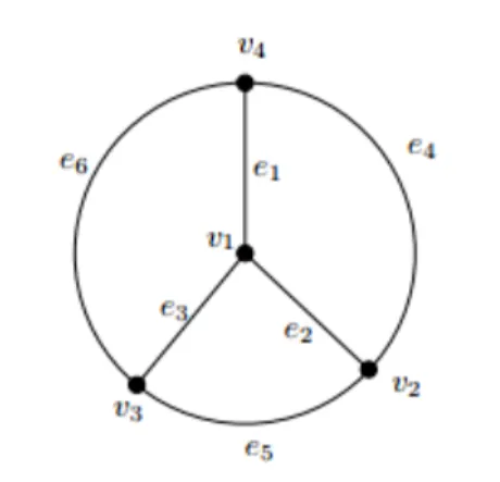
Due to the lack of uniqueness in the description of 4-valent or higher vertices, it is the case that most spin networks can be represented by several wave-functions of the same kind as the one in Figure 2.2.1 — where ψ = (ρj1(he1[A]))α1β1(ρj2(he2[A]))α2β2(ρj3(he3[A]))α3β3C

j1j2j3

β1β2β3.... For example, When

writing the wave function of a spin network where 4 edges (e1 to e4) meet at one vertex, it is necessary 1_{The quantum configuration space is given by the space of holonomies [6].}

(25)

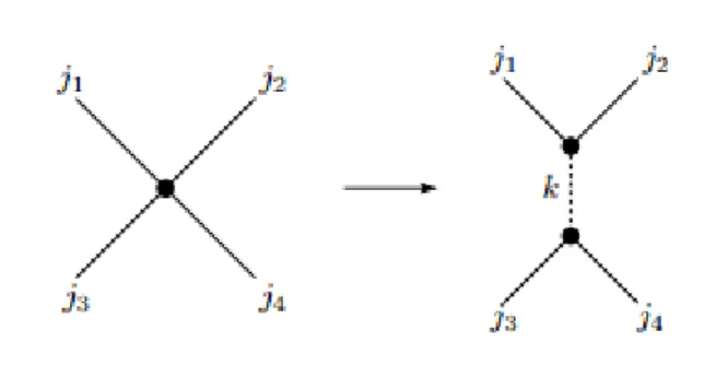
Figure 2.2.2: A 4-valent vertex can be defined as two 3-valent ones and other assignments of pairs of edges (e.g. 1-3, 2-4) are equally possible, provided we use the correct intertwiners in the wave function equation [2].

to group the edges into pairs. Say we choose (1,2) and (3,4). Then the wave function will be similar to the one in Figure 2.2.1 and differ only on the intertwiners, which become Cj1j2k

β1β2βC

j3j4k

β3β4β, where the

spin k can be any chosen value between |j1− j2| and j1 + j2, as expected from quantum mechanics.

Furthermore, we can switch to a different wave function representation by means of a transformation of the Clebsh-Gordan coefficients to the new ones representing the new coupling of the edges. Pictorially, this implies that a 4-valent vertex can be split into two virtual 3-valent vertices, with a virtual edge joining both and having a spin k attached to it, as shown in Figure 2.2.2.

The wave functions are cylindrical and act on the connection A only on a set of measure 0 — anal-ogously to the Dirac delta function acting on other functions [2]. As a result, the Hilbert space of spin networks is given by the linear combinations of these functions over all the graphs, just as stated in (2.1.10). Additionally, the product of two cylindrical functions (even on different spin networks) is a cylindrical function and their scalar product, which is diffeomorphism invariant, vanishes for different graphs, Γ̸= Γ′, and is identical to (2.1.11) for coinciding graphs [2]. Lastly, we define the kinematical Hilbert space in the same manner as the one done earlier, meaning it is composed of all linear superpo-sitions of spin network states Ψnwith finite norm, i.e. Ψ =

∑_∞

n=1anΨn, with||Ψ||2 <∞. The main feature of this Hilbert space, as well as the one which differentiates the approach mentioned here from others, is its non-separability [2].

Spin networks allow us to describe the quantum geometry of space, as it is a description of a quantum state of the gravitational field on a spatial sector Σ of the spacetime manifold. However, for a description of spacetime, i.e. for a description of the evolution of spin networks, we need to ascend one dimension higher and follow the spin foam approach.

(26)

(27)

Chapter 3

Spin Foams

3.1 Overview

As discussed earlier, spin foams are the proposed solution to the problem of defining the dynamics of loop quantum gravity. They arise from the formal definition of the exponentiation of the scalar constraint and this approach can be seen as a path integral formulation of LQG [3]. When dealing with the scalar constraint, one can define the “projection operator” P from the kinematical Hilbert space to the kernel of the physical one [3]. The formal expression is given by

P = ∏ x∈Σ δ( ˆS(x)) = ∫ D[N]ei ˆS[N]_, _{S[N] =}_ˆ ∫ dx3N (x) ˆS(x), (3.1.1)

where N (x) is the lapse function and ˆS is the scalar constraint. When P is applied to any state in the

kinematical Hilbert space, the result is a solution of the set of constraints imposed on Hkin— the scalar, diffeomorphism and Gauss ones —, also called quantum Einstein equations (QEE) [3]. Moreover, apart from allowing us to obtain the space of solutions of the QEEs, this projection operator also defines the inner product for said space, imbuing it with the same structure as Hphys[3].

In the spin network basis (discussed earlier), the matrix elements of P can be thought of as the sum of transition amplitudes of evolving spin networks, in what might be called a quantum history. A graphical representation of this concept is given in Figure 3.1.1, where the spin network slices are clearly visible and similar to the ones in Figure 2.2.1.

More formally, we can designate the transition between two spin network states s and s′ as a spin foam history and describe it by using a 2-complex bounded by these states, F_s_→s′ — such as the one in Figure 3.1.1 —, and a set of spin quantum numbers{j} acting as labels for the edges e, faces f and vertices ν of the complex. As such, the so-called physical inner product is then given by

Pss′ = ⟨ s′, s ⟩ p =⟨P s, s⟩ = ΣF s→s′N (Fs→s′)Σ{j}Πf⊂Fs→s′Af(jf)Πe⊂Fs→s′Ae(je)Πν⊂Fs→s′Aν(jν), (3.1.2)

i.e. it is a sum over the spin foam amplitudes, namely the 2-cell (e), 1-cell (f ) and 0-cell (ν) ones, given respectively by the 3 different Ai in the equation above. The dependence on ji, on the other hand, is referring to the quantum numbers defining the neighbourhood of some edge, face or vertex of F , which in the case of Figure 3.1.1 is specifically written as Aν(j, k, l, m, n, s). Additionally, the remaining N (F ) is a normalisation factor.

(28)

Figure 3.1.1: A spin foam describing the transitions between 3 different spin networks, forming a 2-complex (left), and a transition vertex (right) within the spin foam. The transitions between spin networks occur from bottom to top and, as one can easily notice, with each transition, new links are created and the spins are reassigned at the vertices [3].

The physical interpretation of a spin foam is that of a quantum history of spin network states: a set of transitions between quantum states of space or, equivalently, the evolution of the gravitational field. In other words, spin networks represent space, while spin foams represent spacetime. Furthermore, since the spin assignments give us the degrees of freedom of the gravitational field, they are responsible for representing the geometry of spacetime, not the shape of the spin foam itself. The obvious consequence is the expected background independence, as opposed to the lattices used in quantum field theory, for instance.

It is important to state that spin foams are an approach to the dynamical issue of LQG and thus are merely a tool, not a definitive theory. In fact, one can find numerous different models using the spin foam approach.

3.2 Spin Foam Model Prescription

In order to describe the spin foam approach to 4-dimensional general relativity, we shall follow the pre-scription for the 3-dimensional case [11], not only due to its increased simplicity, but also due to its chronological accuracy, regarding the origin of spin foams. In this 3d case, we have the following action for gravity (with cosmological constant Λ):

S3d= ∫ ϵIJ K ( eI∧ FJ K(ω) +Λ 6e I_{∧ e}J_{∧ e}K ) (3.2.1) (where e≡ B, as shown below).

The above theory is topological, meaning there are no local propagating gravitational degrees of freedom, which entails the fact that it can be discretised. In fact, a refined enough discretisation that takes into account all global degrees of freedom ensures that the new theory is discretisation-independent [11]. As a result, 3d gravity is closely related to the spin foam quantisation and we thus obtain a similar transition amplitude. Applying the above to Riemannian gravity, we obtain the Turaev-Viro model, for Λ > 0, and the Ponzano-Regge (state-sum) model (of 3-dimensional quantum gravity) for Λ = 0.

Next, we move on to 4D and present a theory which exists in any number of dimensions, called BF theory. BF is a topological field theory which naturally gives rise to a topological quantum field theory

(29)

when quantised. Hence, we can use this theory as an intermediate one between 3- and 4-dimensional gravity, in which case we get the action

SBF = ∫

BIJ ∧ FIJ(ω), (3.2.2)

where BIJ is an SO(η) Lie algebra valued (d-2)-form. One can easily check that BIJ = ϵIJ KeK yields the previous case, i.e. 3-dimensional gravity. Additionally, BF theory is also a toplogical theory (in any dimension) and it can be quantised using the spin foam approach, which again provides a discretisation-independent theory.

Now if we use BIJ =∗(eI∧ eJ)(where eI, eJ are tetrads and∗ is the Hodge star operator), we get a correspondence between the Hilbert-Palatini action and the 4d BF theory one, as well as a reduction from the latter to general relativity. The most important concretion of this method is the Plebanski action, which only differs from SBF by one additional term:

SP l = ∫ ( BIJ ∧ FIJ(ω) + 1 2ϕIJ KLB IJ_{∧ B}KL ) . (3.2.3)

Here, ϕ is a field satisfying a number of symmetry constraints, including ϵIJ KL_ϕ

IJ KL = 0. The extra term’s purpose is to impose the simplicity constraints, which are

BIJ ∧ BKL= σVϵIJ KL ⇐⇒ ϵIJ KLBµνIJBρσKL = σVϵµνρσ, (3.2.4) for the (non-degenerate) caseV = _4!1 Tr (B∧ B) ̸= 0. Here, σ denotes the sign which differentiates between Lorentzian and Riemannian cases. These constraints are aimed to reduce BF theory to general relativity, which is achieved because of the fact that the two sets of solutions for the simplicity constraints (for the same aboveV), i.e. BIJ =∗(eI∧ eJ)and BIJ = eI∧ eJ, give the Hilbert-Palatini formulation and the extra term from the Holst action (respectively), when applied to the Plebanski action. These two give the entire Holst action, which is equivalent to the Palatini one, which in turn yields general relativity. Spin foam models for 4D general relativity usually make use of the Plebanski action and quantise the correspondence between BF theory and GR, by first discretising the classical theory (i.e. inserting it into a simplicial complex), then quantising the topological BF part of the new (discretised) theory and finally imposing the simplicity constraints at the quantum level. In other words, we quantise before constraining. Having presented the prescription under which most spin foam models come to be [11], we shall now review a number of them.

3.3 Spin Foam Models

In 1977, Plebanski equated the action of a constrained SU (2) BF theory, below, to that of self-dual general relativity [12, 13, 14]: S(B, A) = ∫ Tr [B∧ F (A)] − ψij [ Bi∧ Bj−1 3δ ij_Bk_{∧ B} k ] . (3.3.1)

The correspondence between both theories is attained when we vary ψij, which gives Ωij = 0, where Ωij is the term being multiplied by ψij, in the equation above. These are the constraints which reduce the action of BF theory to the one of self-dual Riemannian gravity.

(30)

From here, Reisenberger showed that the simplicial discretisation of the aforementioned action is well-defined and said action is recovered when the triangulation is refined [15]. Later on, he formu-lated a spin foam model from this discretisation, by promoting the Bito operators, thereby imposing the constraints Ωij [16]. The resulting model is then

ZGR = ∫ ∏ e∈J∆ dgee− 1 2z2Ωˆ 2 ∑ C:{j}→{f} ∏ f∈J∆ ∆jf Tr [ jf ( g_e1...gN_e )], (3.3.2)

where ˆΩij =Ji∧ Jj−1₃δijJk∧ Jkand the constraints are imposed on a single 4-simplex amplitude, as a form of locality. The exponential function is used in order to impose the constraints sharply in the limit z → ∞ [1], otherwise the algebra of the operators would not close, due to the way in which the constraints are implemented.

A generalisation of Reisenberger’s model is one created by Freidel and Krasnov, in 1999 [14]. Their starting point was the BF action (first term) with an extra polynomial function of the B field (second term):

S(B, A) =

∫

Tr [B∧ F (A)] + Φ(B). (3.3.3)

Here, we can define the partition function Z[J ] as the functional integral over A and B of the exponential function of i∫ Tr [B∧ F (A)] + Tr [B ∧ J], where J is an algebra-valued 2-form — we also discretise the manifold, as with most spin foam approaches. This model is useful for representing theories such as Yang-Mills, BF with cosmological terms or, if we define A and B as SU (2)-valued and Φ as the second term of equation (3.3.1), self-dual Riemannian gravity, as in Reisenberger’s case. However, There are some differences between these two models, namely the fact that Biis now represented by (commutative) functional derivatives, as opposed to (non-commutative) invariant vector fields, or the use of a potential term, instead of constraints.

In the case of Iwasaki [17], the spin foam model is again used for self-dual Riemannian gravity and is obtained by first performing a lattice discretisation of the Ashtekar formulation of general relativity. The consequent discrete action is obtained through a lattice path integral , using the Haar measure.

One of the main innovations in terms of spin foam models came with Barrett and Crane, in 1998. While the above models are closely related to loop quantum gravity, through the use of self-dual Rie-mannian gravity — where we get SU (2) spin network states as boundaries —, they do not produce simple (nor closed) equations [1]. The Barret-Crane model [18, 19], on the other hand, is a much simpler one, based on the quantisation of the simplicial SO(4) Plebanski action and on the concept of the quantum tetrahedron [20, 21]. The latter is essentially an assignment of an irreducible unitary representation of

SU (2) to each face of a tetrahedron, along with the requirement that this polyhedron’s faces must close.

More recently, in 2007, Engle, Pereira, Rovelli and Livine published a modification of the Barrett-Crane model [22, 23, 24] (henceforth known as the “EPRL model”), which relaxes the Plebanski con-straints — which reduce quantum BF theory to general relativity — imposed by the latter and thus is simpler and more closely related to LQG. The main problem with the previous approach was the non-commutativity of the quantum B field (and hence of the simplicity constraints as well), which entails a non-closed algebra, obtained from the commutation of Plebasnki constraints. Since these constraints imply additional classically non-existent (and possibly superfluous) conditions, one is able to relax them, thereby obtaining the simpler EPRL model from Barrett-Crane’s.

Finally, a year later, Freidel and Krasnov developed a very similar model to EPRL [25]. In fact, it is identical to it for an Immirzi parameter γ < 1. This time, however, the approach involved the

(31)

representation of the BF path integral of BF theory in terms of coherent states. As a result, it was possible to implement the Plebanski constraints semi-classically. The EPRL model benefitted from the FK model, by using the linear Plebanski constraints to reach a generalisation to arbitrary γ.

It is interesting to note that the last two models are widely regarded as the most advanced theories of 4-dimensional quantum gravity [1]. As a result, the EPRL model and its semiclassical limit will be discussed in the later sections.

3.4 Quantising BF Theory

Following Perez and Baez [1, 26], we learn that the action of (classical) BF theory is given by

S [B, ω] =

∫

M

⟨B ∧ F (ω)⟩ , (3.4.1)

where G is a compact group with a Lie algebra g having the inner product ⟨⟩, M is a d-dimensional manifold, B is a differential (d−2)-form, with values in g, F is the curvature 2-form and ω is a connection on a G-bundle over the manifoldM. Since all solutions to the equations of motion are locally related by gauge transformations, there are no local excitations within this theory [1]. As gauge symmetries of the action, we have the topological gauge transformation

δB = dωη, δω = 0 (3.4.2)

and the local G gauge transformations

δB = [B, α] , δω = dωα, (3.4.3)

where the dωare just the covariant exterior derivatives of the 0-forms (η and α) with values in g. These symmetries originate from the Bianchi identity (dωF (ω) = 0) and the action above, respectively. Since the equation of motion solutions are pure gauge, it follows that the theory has only topological or global degrees of freedom.

It is interesting to note two special cases of BF theory: Riemannian general relativity, for G = SU (2) and d = 3; and its spin foam 4-dimensional quantisation, for G = Spin(4) and d = 4. The latter can be related to general relativity by constraining the field B_abIJ = ϵIJ_KLeK_aeL_b (where eI_ais the tetrad co-frame), in our BF theory action above. In doing so, we get the action of general relativity in four dimensions.

In order to avoid infinite volume factors (i.e. infrared divergences) within the transition amplitudes, we assume the compactness of G and deal with non-compact groups later on. Having said that, and adding the assumption of a compact and orientable manifoldM, we get the following partition function

Z =

∫

D[B]D[ω] ei S[B,ω] ₌ ∫

D[ω] δ(F (ω)), (3.4.4)

which is the volume of the space of flat connections on the manifoldM. The next step is to replace the manifoldM with an arbitrary cellular decomposition ∆, associated to a dual 2-complex, ∆∗. The latter is comprised of a set of vertices, edges and faces — v, e, f ∈ ∆∗, dual to d-, (d− 1)-, (d − 2)-cells ∈ ∆, respectively. For simplicial decompositions ∆ ofM in 2, 3, and 4 dimensions, we get (dual) 2-complexes (∆∗), whose faces are dual to 0-simplices (vertices), 1-simplices (edges) and 2-simplices (triangles) of the triangulations (∆), respectively.

Considering a triangulation ∆, we obtain the link between the Lie algebra elements Bf, attached to faces of the dual 2-complex (f ∈ ∆∗), and the B field:

(32)

Bf = ∫

(d−2)−cell

B, (3.4.5)

i.e. Bf can be conceptualised as the integral of the (continuous) (d− 2)-form B over the (d − 2)-cell dual to the face f ∈ ∆∗, or, alternatively, as the smearing of said form on the (d− 2)-cells of ∆. Since we know that

∀ f ∈ ∆∗,∃ ! ((d − 2) − cell) ∈ ∆, (3.4.6) we can now label Bf, the discretisation of the B field.

Similarly, we discretise the connection ω by assigning group elements ge ∈ G to edges e ∈ ∆∗, the former representing the holonomy of the connection along the latter, i.e.

ge= P e−

∫

eω_, _(3.4.7)

where P e is the (path-)ordered exponential. We can now write the partition function (or path integral) of the triangulation ∆ ofM as z(∆) =∫ ∏ e∈∆∗ dge ∏ f∈∆∗ dBfeibfUf = ∫ ∏ e∈∆∗ dge ∏ f∈∆∗ δ (ge1. . . gen) , (3.4.8)

where we have used Uf = ge1. . . gen for the holonomy around faces f and we note that this equation is

the discretised version of the previous path integral, presented in equation (3.4.4). Additionally, dge is the Haar measure, while dBf is the Lebesgue one.

One can further modify this equation by using the left-translational invariance property of the Haar measure, as well, as the Peter-Weyl theorem, to obtain

Z(∆) = ∑ C:{ρ}→{f} ∫ ∏ e∈∆∗ dge ∏ f∈∆∗ dρf Tr [ ρf(ge1. . . geN) ] , (3.4.9)

where ρ are irreducible unitary representations of G and the Dirac delta distribution was modified ac-cording to

δ(g) =∑ ρ

dρTr [ρ(g)] , (3.4.10)

as implied by the latter theorem. The next simplification of this expression involves the integration over the connection, where we can use the fact that an edge e is always shared by d faces to conclude that the group elements geoccur in d distinct traces, and thus write the projector

P_inve (ρ1, . . . , ρd) := ∫

dgeρ1(ge)⊗ . . . ⊗ ρd(ge), (3.4.11) onto Inv [ρ1⊗ . . . ⊗ ρd].

Finally, one is able to obtain the spin foam amplitudes of SO(4) BF theory:

ZBF(∆) = ∑ Cf:{f}→ρf ∏ f∈∆∗ dρf ∏ e∈∆∗ P_inve (ρ1, . . . , ρd). (3.4.12) Simply put, the BF amplitude of a 2-complex ∆∗is the sum of the natural contraction of the network of projectors P_inve , over all possible assignments of irreducible representations of G to faces f .

(33)

Chapter 4

The EPRL Model

4.1 Preliminary Model

Until the introduction of a new model by Engle, Pereira and Rovelli [22, 23] — and a subsequent extension by the same authors, in collaboration with Livine [24] —, the most studied one (in the four-dimensional Euclidean framework) was the so-called Barret-Crane (or BC) model [20, 21], which can be summarised as the straightforward result of a set of simplicity constraints being applied to a topological BF quantum field theory. Remarkably, these constraints correspond to the ones used to transform BF theory into general relativity, in their classical limit, and this theory has been shown to yield a number of correct n-point correlation functions, unlike other results from alternative perturbative approaches [22].

Nonetheless, some problems within the Barrett-Crane theory were later pointed out, including the failure of its boundary state space to match that of (non-perturbative) loop quantum gravity, the lack of a well-behaved volume operator and the erroneousness of the low-energy limit of some of the subsequent correlation functions. These problems were attributed to the gauge fixing used and the needlessly strong imposition of the (second-class) simplicity constraints — as mentioned before —, which fully constrains the intertwiner quantum numbers in a way that leads to the troublesome annihilation of physical degrees of freedom [22].

The solution proposed by the authors of the new model involves the discretisation of Euclidean gen-eral relativity through a triangulation, followed by its quantisation and weak imposition of constraints. As a result, we obtain the SO(3) hamiltonian LQG spin network space as the state space of the theory, as well as a new, SO(3)- and SO(4)-covariant vertex amplitude, which may solve the problem of the incorrect BC correlation functions.

The derivation of the EPRL model starts with a fixed 4d triangulation ∆, which contains triangles f , tetrahedra e and 4-simplices v, associated to faces, edges and vertices of the dual 2-complex defining the spin foam, respectively — not unlike what we have dealed with in previous sections. We assign an integer spin jfto each face and a basis element ieof the intertwiner space to each edge. It is helpful to remember that: each edge is adjacent to 4 faces; whose representations are carried by 4 Hilbert spaces; whose tensor product contains, in turn, an SO(3) invariant subspace; whose elements are the aforementioned intertwiners. By fixing the pairing of the 4 faces, we can obtain the basis yielded by the spin of the virtual link and thus get

dim j = 2j + 1 (4.1.1)

(34)

SU (2) ones, of the form (j+_{, j}−_{), in order to obtain the equation}

15j_SO(4)(j_f+, j_f−, i+_e, i−_e) = 15j(j_f+, i+_e)15j(j_f−, i−_e), (4.1.2) which tells us that the Wigner 15j symbol of the SO(4) group — i.e. a function of 15 irreducible repre-sentations of SO(4) — can be expressed as the product of 2 Wigner SU (2) 15j symbols — equivalent to the Clebsch-Gordan coefficients.

Before unveiling the spin foam partition function, we must introduce a linear map f from the space of SO(3) intertwiners between the 2j1, . . . , 2j4 representations to that of the SO(4) ones, between the

(j1, j1), . . . , (j4, j4) representations. We can thus expand f in terms of its linear coefficients in a given

basis, i.e. f|i⟩ = ∑ i+_,i− f_ii+_i−i+, i− ⟩ , (4.1.3)

where said coefficients are written as

f_ii+_i− = , (4.1.4)

i.e. as the evaluation of the spin network above on the trivial connection. Finally, the spin foam partition function of the EPRL model is

ZEP RL = ∑ jfie ∏ f ( dimjf 2 )2∏ v A (jf, ie) =∑ jfie ∏ f ( dimjf 2 )2∏ v 15jSO(4) (( jf 2, jf 2 ) , f (ie) ) =∑ jfie ∏ f ( dimjf 2 )2∏ v ∑ i+e,i−e 15jSO(4) (( jf 2, jf 2 ) , i+_e, i−_e) ∏ e∈v fie i+ei−e (4.1.5)

Aside from having boundary states spanned by cubic graphs coloured with SO(3) spins and inter-twiners, we also note that this theory simply constitutes a modification of the Barrett-Crane one, whose (spin foam) partition function is given by the sum over half-integer spins jf and the amplitude is an SO(4) Wigner 15j symbol, i.e.

ZBC = ∑ jf ∏ f (dim jf)2 ∏ v ABC(jf) (4.1.6) and ABC = 15jSO(4)((jf, jf), iBC). (4.1.7) 18

(35)

It is clear that the intertwiner state space is the differentiating factor between the two models. While both theories draw their intertwiners from the SO(4) intertwiner space between four simple representations,

He = Inv(H(j1,j1)⊗ . . . ⊗ H(j4,j4)), (4.1.8)

the Barrett-Crane model only uses one intertwiner,

|iBC⟩ = ∑

j

(2j + 1)|j, j⟩ ∈ He, (4.1.9)

whereas the EPRL one uses the states given by the map f|i⟩ above, which span a subspace Ke⊂ He. In other words, while Barrett and Crane completely constrained the intertwiner degrees of freedom, the au-thors of the new model let them remain unconstrained and thus, instead of having a single intertwiner, we now have the space Ke. The reason for this change is the fact that the off-diagonal simplicity constraints need not be imposed strongly — as done by Barrett and Crane, where such imposition on Heresulted in the single|iBC⟩ —, since they do not commute and are hence second-class. In fact, doing so has been shown to eliminate physical degrees of freedom in any given model.

To give a more formal perspective on this idea, we present the pseudoscalar SO(4) Casimir operator for a given pair of faces f ̸= f′sharing an edge

Cf f′ = ϵIJ KLBfIJBKLf′ (4.1.10) on the

(

H(jf,jf)⊗ H(jf ′,jf ′)

)

representation, where ϵ is the totally antisymmetric tensor, the Bs are the generators of SO(4) (with I, J = 1, 2, 3, 4) and the Einstein summation convention is implicit. The off-diagonal simplicity constraints are then

Cf f′ = 0 (4.1.11)

and follow from the fact that the external product of the bivectors of the faces of a tetrahedron (i.e.

Bf1. . . Bf4) vanishes. Nonetheless, due to the aforementioned problems regarding the strong imposition

of such constraints, the authors of the (new) EPRL model opted to rewrite them, before imposing them weakly. Since the constraints simply mean that the tetrahedron must lie on a 3d subspace of 4d spacetime, we automatically get a normal to the tetrahedron, which can be defined as the timelike vector nI = (0, 0, 0, 1), without loss of generality. The result is then

∃n : C = 2C4− C3 = BIJf BfIJ − B ij fB

ij

f = 0,∀f (4.1.12)

where i, j are spatial coordinates and C4 and C3 are the quadratic Casimir operators of SO(4) and

SO(3)≤ SO(4), respectively. Naturally, imposing these constraints will generate a space from

(

H(j_f1,j_f1) ⊗ . . . ⊗ H(j_f4,j_f4) )

,

which yields Ke when projected onto the SO(4) invariant-tensor space. Lastly, the coupling of the antisymmetric nature of the constraints and the symmetric nature of the f|i⟩ states is what ensures that the former vanish weakly.

Having presented the EPRL model and compared it to the previous one, we shall establish the connec-tion between the former and the quantisaconnec-tion of discretised general relativity, as well as the loop quantum gravity framework.

(36)

The first step towards this goal is to discretise general relativity on a Regge geometry, by using a simplicial decomposition ∆. Said geometry should be flat on each 4-simplex and thus allow for the curvature to be located on the “bones” (f ). In fact, the (SO(4)) curvature associated to the triangle f within the tetrahedron t is encoded on the “link” of each bone and is represented by the rotation matrix

Uf(t), defined below. The remaining tools needed for the quantisation are:

• 4-simplices, tetrahedra t and triangles, respectively dual to vertices v, edges (e) and faces f , in the dual 2-complex;

• co-tetrad one-forms e, covering each t and v ; • Bf(t) =

∫

f⋆(e(t)∧ e(t)) ∈ g = SO(4), ∀f ∈ t, where ⋆ is the R

4_{Hodge star operator and g is}

the algebra;

• Group elements Vvt= Vtv−1∈ G = SO(4).

Furthermore, we also assume that, prior to varying the action, we have, for all f ,

Bf(t)Uf(t, t′) = Uf(t, t′)Bf(t′), Uf(t, t′) = Vtv1Vv1t1Vt1v2. . . Vvnt′, t, t

′_{∈ Link(f), (4.1.13)} where the product of V s is around the link of f , from t to t′(clockwise), as shown. The bulk action of e is then the sum over the faces of the trace of the product of Bf, Vtvand Vvt′. Additionally, the boundary terms are obtained by substituting the latter two terms by Uft, t′.

We must now apply the constraints on the chosen independent variables Bf — instead of the tetrads —, ∀f, f′ ∈ t: the aforementioned simplicity constraints and the closure constraint. While the former can now be written as

Cf f′ =∗Bf(t).Bf′(t) = 0, (4.1.14) in both diagonal (f = f′) and off-diagonal (f ̸= f′) cases, the latter deems the sum of Bf over the faces of a tetrahedron to vanish, i.e.

∀t,∑ f∈t

Bf(t) = 0. (4.1.15)

The dot represents the scalar product of the algebra and we also note the existence of an extra “dynamical simplicity constraint” — pertaining to triangles within the 4-simplices —, which is made obsolete when the remaining ones are satisfied.

In practice, While the closure constraint imbues the tetrahedra with gauge invariance and gives us the SO(4) spin network states of the dual graph to the boundary triangulation as our state space, the simplicity ones — as discussed above — output a simple SO(4) representation for each link, as well as Ke as the intertwiner space. Moreover, due to the correspondence between the boundary elements and those of the SO(4) lattice gauge theory, we are able to the define the latter’s Hilbert space as our (unconstrained) own.

The last steps towards obtaining the EPRL model’s partition function involve the amplitude of a 4-simplex (A[Btt′]) expressed in terms of the conjugate variables, i.e.

A[Utt′] = ∫ dBtt′e−i ∑ Tr[Btt′Utt′]_A[B tt′], A[Btt′] = ∫ dVvtei ∑ Tr[Btt′VtvVvt′]_, _(4.1.16) 20

Semiclassical limit of the EPRL spin foam model