Rio de Janeiro, Brazil, 01 - 05 July 2012.
Analysis of diverse optimisation algorithms for pump scheduling in water supply systems
B. Coelhoa,*, A. Tavaresa and A. Andrade-Camposaa
Department of Mechanical Engineering, Centre for Mechanical Technology & Automation, GRIDS research group University of Aveiro, Campus Unversitário de Santiago, 3810-193 Aveiro, Portugal
1. Abstract
Nowadays, the major expenses with water supply systems (WSS) correspond to energy consumption. The number of scientific works dealing with operational optimisation in WSS has been increasing over the past years, demonstrating significant reductions on energy costs and consumption. Pump stations usually represent the major portion of total energy costs in WSS. Consequently, in this work, it is pretended to give a contribution for energy efficiency improvement in pump stations. Generally, in WSS, the pumps are switched on when the reservoirs, responsible for supplying certain populations, reach their minimum levels. These pumps are only switched off when the reservoirs reach their maximum levels. The introduction of an operational pump pattern adapted to the energy tariff variation and the consumption patterns of the populations can optimise pump stations operations, minimising energy costs significantly. However, the process of finding the best pattern can present difficulties due to the complexity of some WSS (multiple pumps, multiple reservoirs, nonlinear behaviour of the systems, etc).
In this work, an interface was developed with the aim of applying different optimisation algorithms for pump scheduling in WSS. The interface makes an automatic connection between a hydraulic simulator (EPANET 2.0) and the different optimisation algorithms selected, providing, after multiple iterations and evaluations, an optimal pump pattern for a certain water supply network represented. Two different examples of water supply networks are introduced in this study in order to validate the developed methodology. For both WSS, classic and meta-heuristic optimisation algorithms are tested and analysed.
2. Keywords: Cost Reduction, Energy Efficiency, Optimisation Algorithms, Pump Scheduling, Water Supply Systems (WSS).
3. Introduction
Water supply and distribution systems should satisfy the requirements of several consumption sectors, responding to the demand in each place and time and with appropriate pressures [1]. Although the large size variation and complexity of water distribution systems, they all have the goal of deliver water from the source to the consumer [2] at adequate pressures and quantity.
Generally, a WSS comprises four main sections [3]: (i) water sources and intake works, where the water extraction is made by the intake structures and pumping stations; (ii) treatment works and storage, (iii) transmission mains (pumping and/or gravity), where the bulk water is transported to the treatment plants and then to the storage reservoirs; and (iv) the distribution network which delivers water to consumers through service connections. The distribution networks configuration can be looped, branched or, as in most of cases, mixed (a combination of looped and branched networks). Branched networks only enable one flow direction whereas looped networks, with connected pipes that constitute loops, allow changes in flow direction according different demands in each node. The main advantage of the looped configuration is the guarantee of water supply when some pipe break occurs (for maintenance, for example). Another advantage of looped networks is related with the lower velocities (due to the existence of more than one path for water) that enlarge the system capacity [2].
The main components of a water supply system are [1]: pipes, junctions, storage reservoirs (or variable level reservoirs), water sources (or fixed level reservoirs), pumps and valves. Pumps are essential components on energy efficiency studies of WSS.
A pump is a device that transfers the mechanical energy to the fluid as hydraulic head. This head, called pump head, is a function of the flow that passes through the pump. Thus, the pumps are used when the WSS needs energy to overcome elevation differences. Centrifugal pumps are the mostly used in this kind of system [2]. The relationship between pump head and pump discharge is represented by the pump head characteristic curve. This is a nonlinear curve that shows a decreasing head with the flow rate through the pump. Pumps can be of constant or variable speed and should operate inside the limits imposed by the characteristic head curves. In variable-speed pumps, the pump discharge is directly proportional to pump speed and the pump head is proportional to the square of the speed [2].
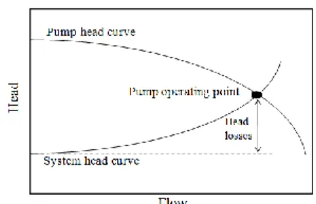
Another important issue about the pumps is the operating point (or nominal work point) given by the crossing point between the pump head curve and the water system resistance curve (see Figure 1). The operating point represents the discharge that will pass through the pump and the head that will be added by the pump [2]. When the system head variation or the water demand variation occurs, the pump can operate outside the nominal work point but with lower efficiency conditions [4].
The fast expansion of several water supply systems due to the population growth and the immediate consumers supply without any planned strategy have led to inefficiently operated systems. In these systems, pump stations usually represent the main operational costs [5,6] revealing an important opportunity for the efficiency improvement of the water supply systems. In fact, the demand by industry to control pump systems efficiently has been increasing.
Pump stations can be controlled according to variations in suction pressure or even by time controls [7]. However, in most of cases, pumps are controlled by the reservoirs water level variations. In these cases, pumps are only switched on when the reservoirs responsible for supply certain populations are in their minimum levels and switched off when the same reservoirs reach their maximum levels. If the pumps operate according to the variation of the energy tariff during a day, the associated costs could be significantly reduced [8].
Figure 1. Definition of the pump operating point.
This paper explores the application of operational optimisation in water supply systems in order to minimise costs, more specifically the optimisation of the pumping systems operations.
A methodology to apply different optimisation algorithms in order to reduce energy costs associated to the water pumping is presented in a case study. Two different examples of water supply networks were used to test the developed methodology. For the simulation and evaluation of the behaviour of both WSS examples and also to obtain the daily costs of the water pumping, the EPANET 2.0 was applied. EPANET is a computer programme that performs extended period simulation of hydraulic and quality behaviour within pressurised pipe networks [9]. This hydraulic simulator presents a robust model with a large community of users in the world [1].
4. Operational optimisation
Optimisation problems can be solved using conventional trial and error methods or more effective optimisation methods. In most water supply systems, the optimisation process by trial and error methods can present difficulties due to the complexity of these systems: multiple pumps, valves and reservoirs, head losses, large variations in pressure values, several demand loads, etc. For this reason, innovative optimisation algorithms are becoming more widely explored in the optimisation of the water supply systems. Operational optimisation models have been developed since the eighties, exploring several optimisation techniques such as the most traditional (i) Linear Programming [10,11,12] and (ii) Nonlinear Programming [11,13,14,15,16], but also the heuristics derived from nature like (i) Genetic Algorithms [17,18,19,20,21], (ii) Simulated Annealing [19,22], (iii) Ant Colony Optimisation [23], etc. Genetic Algorithms and mainly Hybrid Genetic Algorithms [24,19] have standing out for their strong ability to solve optimisation problems with high level of nonlinearity and also for their performance dealing with the multi-objective optimisation perspective. The optimisation of the WSS operation consists in find the best strategies for the control elements minimising the total costs while satisfying the consumers demand in terms of flow and pressure conditions [13]. In several scientific works, the operational optimisation problem is treated as a single-objective problem consisting in the minimisation of the operational costs and the use of constraints to satisfy the WSS requirements. However, other works look into this kind of problem as a multi-objective optimisation problem: minimisation of costs and maximisation of hydraulic benefits [20,21,24].
An operational optimisation strategy can also be static or dynamic when real-time systems are used simultaneously [25]. Real-time strategies allow optimal operational adjustments to possible variations in the networks like sudden fluctuations in the demand. A large number of real-cases applications with real-time strategies were already published [18,26,27,28,15]
In the literature, there are essentially two kinds of explicit pump schedule optimisation problems: (i) the most common deals with constant speed pumps, where only two optimisation variables are considered for the pump operation (with the values 1 or 0, usually representing the pump status switched on or switched off), and (ii) the other deals with variable speed pumps, where the values of the optimisation variables are defined by the set of speeds of the pump. Some works also investigate the operational optimisation of the pumping systems through the perspective of the reservoirs (implicit representation of pump schedules), where the decision variables are the reservoir levels variation [10,11,5].
Typically, to solve this kind of problem, simulation periods of 24 hours with 1 hour time-steps are used. However, a recent study dealing with quarter-hourly operation was published [29]. The model presented in this study handles hydropower reservoirs with pumped storage plants. The authors believe that this procedure could be one of the keys to make this kind of problem easier to solve. Firmino et al. [12] used a two-stages optimisation method based on Linear Programming and Integer Linear Programming by an optimisation toolbox of MATLAB 7. This method was applied to Campina Grande WSS in Brazil, which contains three pumping stations and has saved around 15% of the costs and energy consumption. Constraints in the reservoirs levels were considered. A case study in China of a large-scale WSS [19] demonstrated a reduction on energy costs of 6.04% using a Hybrid Genetic Algorithm (Genetic Simulated Annealing, GSA). The developed methodology uses an objective function which considers not only electricity cost of pump stations but also the water production cost.
Zyl et al. [5] also developed a hybrid optimisation strategy, combining a Genetic Algorithm with two Hill Climber methods: (i) Fibonacci coordinate search and (ii) Hooke and Jeeves pattern search. In their study, the optimisation variables were defined in terms of tank level controls. A pump penalty cost and a tank penalty cost were used to impose the system constraints. These penalties were determined by a trial and error approach. The developed methodology was applied to the Richmond WSS in U.K. The hybrid method proved to be superior to the pure GA, reducing more than 25% the operating costs.
The POWADIMA research project [18] has developed a real-time methodology which combines the use of an Artificial Neural Network (ANN) for predicting the consequences of different pump and valve control settings (hydraulic equilibrium) and a GA optimiser for selecting the best combination. Constraints to pressures, flow velocities and reservoirs levels were also included. This methodology was tested in the Haifa-A WSS of Mount Carmel, reducing energy costs in 25% [26] and also in Valencia WSS
(Spain), indicating a potential operational cost saving of 17.6% [27].
In Madeira (Portugal), the Socorridos WSS, a system with water consumption and inlet discharge, was tested with the methodology proposed by Vieira et al. [11]. The authors used Linear Programming and Nonlinear Programming tools for the operational optimisation and EPANET for the hydraulic simulation. Savings of nearly 100€/day were obtained with the Nonlinear Programming approach and when a wind park is added to the system, the profits are approximately 5200€/day.
The previous real-cases presented are just some of the many examples of the successfully application of diverse optimisation methodologies in pump systems operation.
5. Case Study
In this section, a case study with two distinct water supply networks is presented. The main objective of the study is to test the behaviour of two different algorithms for the pump schedule optimisation: (i) the Levenberg-Marquardt, a gradient-based algorithm and (ii) an Evolutionary Algorithm, based in the natural evolution of the species.
5.1. Problem Formulation
An optimisation problem is a mathematical model whose main objective is to minimise (or maximise) something through an objective function [10]. The main goal in the presented study is to minimise the costs associated to water pumping in a WSS. The decision variables are given by a pump pattern during one day divided into 24 time intervals of one hour, therefore corresponding to 24 variables. Mathematically, the presented problem can be represented by the general formulation of an optimisation problem:
subject to (1)
where is the objective function, i.e. the pumping energy cost for a day, represent the decision variables given by the set of pump speeds (in this case ) and is a constraint function that depends on the pump operation. The value of the constraint function is zero if the simulation is well succeeded or one if some warning* appears during the simulation. To solve the errors that make appear these warnings, the exterior penalty method† is used at each iteration. In a simplified form, the objective function modified by the exterior penalty method can be expressed by:
(2)
where is the penalty coefficient that was considered fix and equal to ‡.
5.2. Implementation
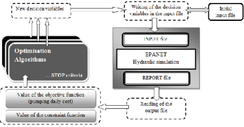
The process of testing the behaviour of each WSS with the replacement of the corresponding pump pattern in order to obtain the minimum energy cost is very time consuming due to the large number of decision variables. For this reason, an interface in C++ that makes this process automatic was developed (see Figure 2).
Figure 2. Scheme describing the developed methodology.
The presented methodology starts with an initial input file containing all the characteristics of the WSS that is supposed to optimise. The input file is sent to EPANET in order to run the hydraulic simulation and a report file is then provided. The interface proceeds to the reading of some values present in the respective file such as the value of the objective function and the constraint function. These values are sent to the optimisation module and new decision variables are provided by the optimisation algorithm. The new variables replace the first one in the input file and a new hydraulic simulation will run. This cycle previously described is repeated until reach the stop criteria.
* The main warnings that can occur are: negative pressures, impossibility in solve hydraulic equations, equilibrium conditions not satisfied or even the pump shutdown when operating outside de range of values of its characteristic curve. Pump patterns that reproduce this kind of errors (solutions not admissible) can never be accepted in order to ensure the correct operation of the WSS.
† Exterior penalty methods can be applied in problems with equality and/or inequality constraints. ‡
5.3. Water Supply Systems Description
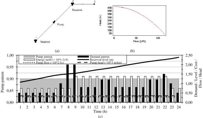
In this section, the simulation of two distinct water supply systems and their initial characteristics are presented and analysed. One of the presented examples is an intuitive system due to its simplicity, which facilitates the analysis of results. This basic network, represented in Figure 3(a), is composed of two reservoirs and one pump. Pump 1 is responsible for pumping the water from the reservoir 1 with an elevation of 50 m to the reservoir 2 with 400 m of elevation. The stored water in reservoir 2 supplies the population represented by node 3 with an elevation of 300 m and a base demand of 10 l/s. The reservoirs 1 and 2, with a diameter of 100 m and 40 m respectively, have a minimum level of 0.5 m and a maximum level of 5 m. Their initial levels are, respectively, 1 m and 2 m. The pump presents an optimum operational point for 350 m of head at a flow of 60 l/s. Its characteristic curve is represented in Figure 3(b). In this figure, it is observed that the pump does not have a linear behaviour with the flow variation, which is an evidence of the nonlinearity of the proposed problem.
The main initial characteristics of the basic system for a one day simulation period and the energy tariff considered are presented in Figure 3(c). With the constant pattern attributed to the pump, it is possible to see that, during all the simulation period, the flow provided by the pump (around 30 l/s) exceeds the water demand of the population. Consequently it is observed a gradual increase on the reservoir level.
Figure 3. Basic Water Supply System: (a) scheme of the network, (b) characteristic curve of the pump and (c) main characteristics of the system for a time horizon of one day (24 hours).
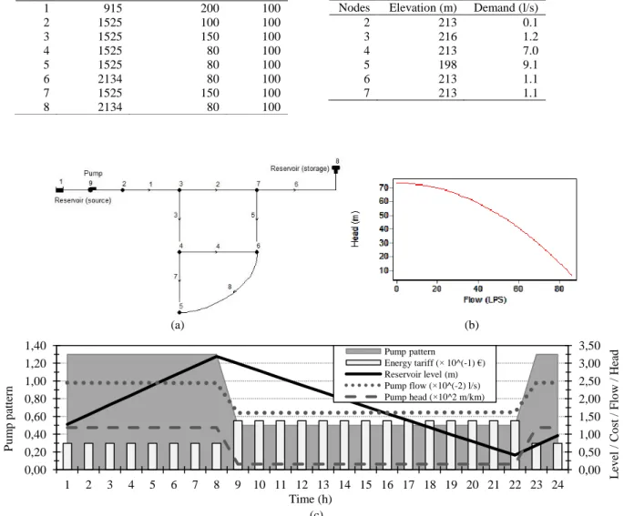
In order to test the developed methodology in a more complex system, a meshed water supply network was simulated for the same time horizon. This network, represented in Figure 4(a), presents two loops and is composed by one reservoir (water source) with an elevation of 213 m, one storage reservoir with 253 m of elevation and one pump responsible for pumping the water from the source to all points of consumption (nodes). The storage reservoir, with a diameter of 9 m, presents an initial level of 1 m. Its minimum and maximum levels are, respectively, 0 and 6 m. The elevations and consumptions that characterise each node of the system as all the pipes dimensions are described in Tables 1(a) and 1(b). The pump of this system can deliver 57.5 m of head at a flow of 18 l/s. Its characteristic curve can be consulted in Figure 4(b).
For the hydraulic simulation of the two-loop WSS with EPANET 2.0, the Hazen-Williams formula was selected with the aim of include pipe head losses on the system§. The initial characteristics of this system are represented in Figure 4(c). In this case, it was
chosen a different initial pump pattern, adapted to the energy price variation during the day. So it is possible to see that in the period between the 8th and 22th hours (higher energy price), the storage reservoir is emptying due to the reduced flow provided by the pump.
§ Note that these head losses contribute to increase the nonlinearity of the system.
(a) (b) (c) 0,00 0,50 1,00 1,50 2,00 2,50 0,80 0,85 0,90 0,95 1,00 1 2 3 4 5 6 7 8 9 10 11 12 13 14 15 16 17 18 19 20 21 22 23 24 De m an d / L ev el / Co st / F lo w / He ad P u m p p att ern Time (h)
Pump pattern Demand pattern
Energy tariff (× 10^(-1) €) Reservoir level (m) Pump flow (×10^2 l/s) Pump head (×10^3 m/km)
Table 1. Properties considered for (a) pipes and (b) nodes of the two-loop water supply system. C-Factor corresponds to the coefficient of the Hazen-Williams formula to calculate pipe head losses.
Figure 4. Two-loop Water Supply System: (a) scheme of the network, (b) characteristic curve of the pump and (c) main characteristics of the system for a time horizon of one day (24 hours).
The values for the daily costs and energy consumption associated to the water pumping in both WSS previously described can be consulted in Table 2. Analysing the table, it can be seen that, in the case of the basic WSS, there is no significant difference between the maximum and the average power required by the pump. This is because the pump always needs the same power to overcoming the difference on elevation between the two reservoirs. In respect to the two-loop WSS, there is a difference between the values of the maximum and the average power required by the pump. Due to the existence of two loops on the system, at a specific period of the day (high energy price), the change of the flow direction in some pipes occurs when the storage reservoir is providing water to the network. Thus, in this situation, the power required by the pump decreases because is not necessary to provide water to all the nodes.
Table 2. Initial values for the daily cost and energy consumption as for the maximum and average power required in the water supply systems of this study.
System Energy consumption (kWh/m3) Average power (kW) Maximum power (kW) Daily cost (€) Basic WSS 1.27 134.79 136.48 242.26 Two-loop WSS 0.21 17.75 37.96 34.61 (a) (b) (c) 0,00 0,50 1,00 1,50 2,00 2,50 3,00 3,50 0,00 0,20 0,40 0,60 0,80 1,00 1,20 1,40 1 2 3 4 5 6 7 8 9 10 11 12 13 14 15 16 17 18 19 20 21 22 23 24 L ev el / Co st / F lo w / He ad P u m p p att ern Time (h) Pump pattern Energy tariff (× 10^(-1) €) Reservoir level (m) Pump flow (×10^(-2) l/s) Pump head (×10^2 m/km) (b)
Nodes Elevation (m) Demand (l/s)
2 213 0.1 3 216 1.2 4 213 7.0 5 198 9.1 6 213 1.1 7 213 1.1 (a)
Pipes Length (m) Diameter (mm) C-Factor
1 915 200 100 2 1525 100 100 3 1525 150 100 4 1525 80 100 5 1525 80 100 6 2134 80 100 7 1525 150 100 8 2134 80 100
6. Optimisation Results
In this section, the optimisation results of the case study are presented and discussed. 6.1. Basic Water Supply System
The results obtained with the optimisation of the basic WSS, using the Levenberg-Marquardt method (LM) and the Evolutionary Algorithm (EA), are presented in Table 3.
As the EA are probabilistic, it is not usual to obtain the same final result in consecutive executions. For this reason the algorithm was executed 6 times and the average value was considered.
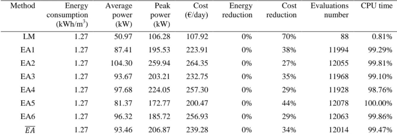
It is observed in Table 3 that the LM was the most efficient method, reducing the pumping costs 70% in just 88 evaluations, presenting the lowest CPU time. On the other hand, the performance of the EA was not as good as the LM. The EA took an average of 12014 evaluations of the objective function which has resulted in a larger CPU consuming with lower cost reductions.
It was expected, in this kind of problem, a better performance with the EA. However, that was not observed. The objective function probably corresponds to a smooth and convex function and thus best results were obtained with the classic gradient-based method. Table 3. Values obtained with the optimisation of the basic water supply system with the Levenberg-Marquardt method (LM) and the
Evolutionary Algorithm (EA). Method Energy consumption (kWh/m3) Average power (kW) Peak power (kW) Cost (€/day) Energy reduction Cost reduction Evaluations number CPU time LM 1.27 50.97 106.28 107.92 0% 70% 88 0.81% EA1 1.27 87.41 195.53 223.91 0% 38% 11994 99.29% EA2 1.27 104.30 259.94 264.35 0% 27% 12055 99.81% EA3 1.27 93.67 203.21 232.75 0% 35% 11968 99.10% EA4 1.27 97.68 224.05 257.30 0% 29% 11928 98.76% EA5 1.27 81.37 172.77 200.47 0% 44% 12078 100.00% EA6 1.27 96.32 185.72 256.93 0% 29% 12063 99.86% 1.27 93.46 206.87 239.28 0% 34% 12014 99.47%
The evolution of the objective function value for each applied method and the comparison of both are presented in Figure 5.
In the case of the LM method (Figure 5(a)), the existence of some peaks in the value of the objective function, corresponds to the occurrence of errors during the simulation. As the variables responsible for these values should not be accepted, the corresponding iterations were removed. Thus, the improved function evolution was also represented. For the first 25 iterations there are no variations in the function value because in this method those iterations are needed for the derivative calculations. After these iterations it is observed a faster convergence of the function to the minimum value.
In respect to the function evolution for the EA (Figure 5(b)) the convergence is not so fast. Moreover, each execution presents different convergences. This corresponds to expected results for this kind of method.
Figure 5. Evolution of the objective function value during the optimisation process of the basic water supply system with (a) the Levenberg-Marquardt method and (b) the Evolutionary Algorithm.
(a) (b) 100 200 300 400 50 150 250 350 450 550 650 1 4 7 10 13 16 19 22 25 28 31 34 37 40 43 46 49 52 55 58 61 64 67 70 73 76 79 82 85 88 f(x ) im p ro v ed f(x ) Iteration f(x) f(x) improved 150 250 350 0 200 400 600 800 1000 1200 1400 1600 1800 2000 f(x ) Generation
EA1 EA2 EA3 EA4
In order to analyse how the optimised system works, it is presented in Figure 6 the main characteristics of the system optimised with the different methods.
Figure 6. Characteristics of the optimised basic water supply system (a) with the Levenberg-Marquardt method and (b) with the Evolutionary Algorithm (the best values obtained, EA5, were selected).
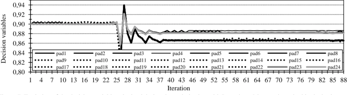
Figure 7. Evolution of the decision variables obtained during the optimisation with Levenberg-Marquardt method in the basic water supply system.
Comparing the optimised pump pattern presented in Figure 6(a) with the evolution of the decision variables in LM method (Figure 7), it is observed an existence of two paths that are followed by the variables values according to the energy tariff (peak and off-peak periods). Although the lowest pump flow during the 22th to 8th hours period, this still exceeds the required by the populations, so the reservoir is filling during this period of time. On the other hand, during the peak period (8-22h), the pump flow is not enough to supply the population and the reservoir is emptying.
Analysing the optimisation with the EA, in Figure 6(b) it is observed almost a random distribution of the variables that constitute the pump pattern. As in these methods the probability of best-fit variables being chosen is higher, it is expected, with the increase of the number of generations, a tendency of the pump pattern to the same obtained with the LM. However the resulting CPU time could not be viable when compared with the LM case.
6.2. Two-loop Water Supply System
The results for the optimisation of the two-loop water supply system are presented in Table 4. For this example there was observed that the average of the values obtained for the EA (10% of reduction in energy and 11% of reduction in costs) is very similar to the
0,80 0,82 0,84 0,86 0,88 0,90 0,92 0,94 1 4 7 10 13 16 19 22 25 28 31 34 37 40 43 46 49 52 55 58 61 64 67 70 73 76 79 82 85 88 De cisio n v ariab les Iteration
pad1 pad2 pad3 pad4 pad5 pad6 pad7 pad8
pad9 pad10 pad11 pad12 pad13 pad14 pad15 pad16
pad17 pad18 pad19 pad20 pad21 pad22 pad23 pad24
(a) (b) 0,00 0,01 0,01 0,02 0,02 0,03 0,03 0,04 0,04 0,85 0,86 0,87 0,88 0,89 1 2 3 4 5 6 7 8 9 10 11 12 13 14 15 16 17 18 19 20 21 22 23 24 D em an d / L ev el / Co st / F lo w / He ad P u m p p att ern Time (h) Pump pattern Demand pattern (×10^(-2)) Energy tariff (×10^(-1) €) Reservoir level (×10^(-2) m) Pump flow (×10^(-3) l/s) 0,00 0,05 0,10 0,15 0,20 0,25 0,30 0,35 0,40 0,45 0,83 0,84 0,85 0,86 0,87 0,88 0,89 0,90 0,91 0,92 0,93 1 2 3 4 5 6 7 8 9 10 11 12 13 14 15 16 17 18 19 20 21 22 23 24 De m an d / L ev el / Co st / F lo w / He ad P u m p p atter n Time (h)
Pump pattern Demand pattern (×10^(-1)) Energy tariff (€) Reservoir level (×10^(-1) m) Pump flow (×10^(-2) l/s) Pump head (×10^(-3) m/km)
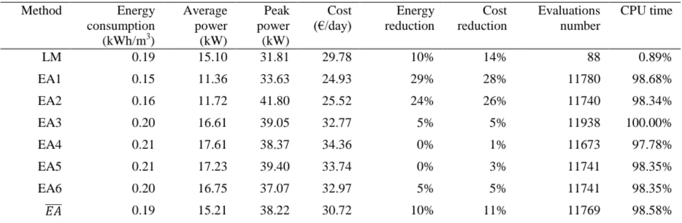
values obtained with the LM (10% of reduction in energy and 14% of reduction in costs). However, the LM method presents less time consume. Observing the first two executions of the EA (EA1 and EA2), it is seen that better reductions of energy and associated costs are achieved.
In this case, both algorithms present a good performance. However the results with the EA probably could be improved if the number of executions were increased.
With the aim of understand better how each algorithm works during the optimisation process, it is presented in Figure 8 the evolution of the values of the objective function.
For the two-loop system, the behaviour of the optimisation algorithms during the simulation is similar to the basic system. In this example, it is also observed the existence of some peaks in the LM function evolution, corresponding to variables not acceptable in the problem. Solving this, it is observed a faster convergence of the LM method when compared with the EA.
Table 4. Values obtained with the optimisation of the two-loop water supply system with the Levenberg-Marquardt method (LM) and the Evolutionary Algorithm (EA).
Method Energy consumption (kWh/m3) Average power (kW) Peak power (kW) Cost (€/day) Energy reduction Cost reduction Evaluations number CPU time LM 0.19 15.10 31.81 29.78 10% 14% 88 0.89% EA1 0.15 11.36 33.63 24.93 29% 28% 11780 98.68% EA2 0.16 11.72 41.80 25.52 24% 26% 11740 98.34% EA3 0.20 16.61 39.05 32.77 5% 5% 11938 100.00% EA4 0.21 17.61 38.37 34.36 0% 1% 11673 97.78% EA5 0.21 17.23 39.40 33.74 0% 3% 11741 98.35% EA6 0.20 16.75 37.07 32.97 5% 5% 11741 98.35% 0.19 15.21 38.22 30.72 10% 11% 11769 98.58%
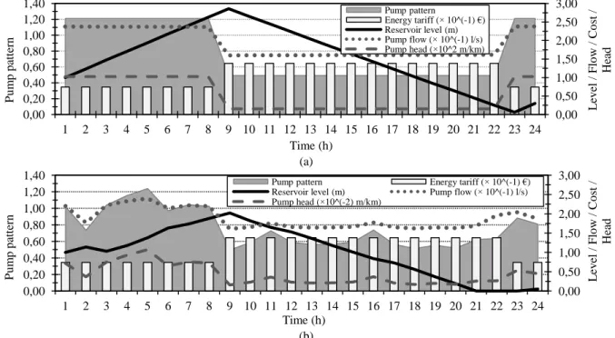
In Figure 9 it is presented the main characteristics of the two-loop system optimised by the LM method and by the EA. In this system, similar characteristics with the basic optimised system are also observed. With the LM method, the variables are exactly according to the energy price variation during the simulation period (see Figure 9(a) and Figure 10). In the optimisation with the EA, the final variables are not as random as in the previous example. It is possible to see the pumping operation according to the variation of the energy price.
Figure 8. Evolution of the objective function value during the optimisation of the two-loop water supply system with (a) the Levenberg-Marquardt method and (b) the Evolutionary Algorithm.
(a) (b) 25 30 35 40 0 200 400 600 1 4 7 10 13 16 19 22 25 28 31 34 37 40 43 46 49 52 55 58 61 64 67 70 73 76 79 82 85 88 f(x ) im p ro v ed f(x ) Iteration f(x) f(x) improved 22 26 30 34 38 0 100 200 300 400 500 600 700 800 900 1000 1100 1200 1300 1400 1500 1600 1700 1800 1900 2000 f(x ) Generation EA1 EA2 EA3 EA4 EA5 EA6 EA avg
Figure 9. Characteristics of the two-loop water supply system after optimisation (a) with the Levenberg-Marquardt method and (b) with the Evolutionary Algorithm (the best values obtained, EA1, were selected).
Figure 10. Evolution of the decision variables obtained during the optimisation with the Levenberg-Marquardt method in the two-loop water supply system.
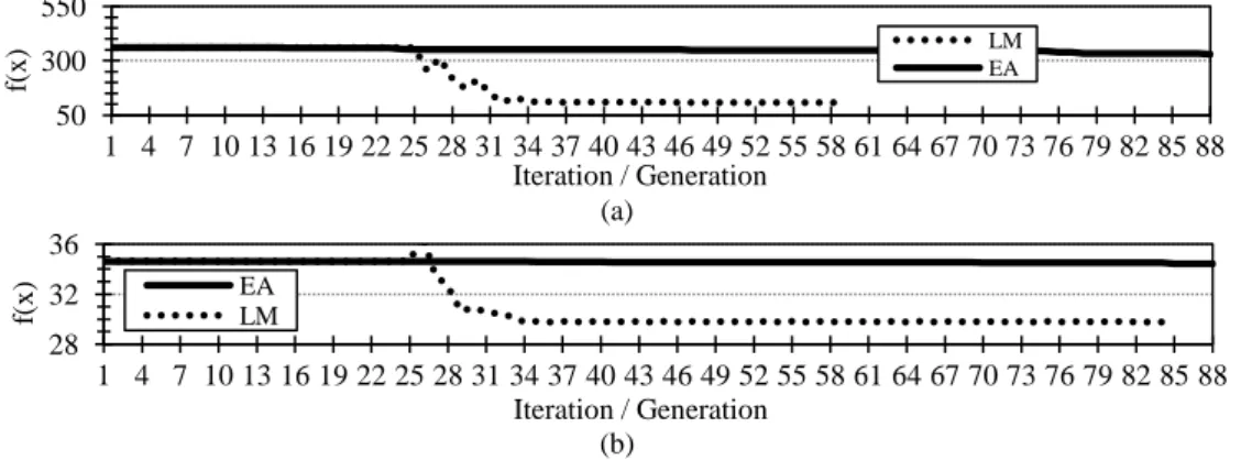
6.3. Results comparison
The results obtained in both WSS tested can be compared by the analysis of the Table 5. The LM method, in both WSS examples, presents the best performance with higher reductions in a significant reduced number of iterations. Figure 11 shows the clear difference between convergences of both selected methods in the two systems.
About EA in the two-loop system, although the average values obtained, in some executions of the algorithm there were observed great values of energy and costs reduction (29 % and 28 % respectively).
Globally, the reductions in energy costs were better in the basic system. As the two-loop WSS is more complex and includes head losses, the optimisation problem becomes more difficult to solve due to the higher level of nonlinearity.
Table 5. Comparison of the optimisation results obtained in both examples of water supply systems. WSS Method Energy reduction Cost reduction Evaluations number
Basic LM 0% 70% 88 0% 34% 12014 EAmax 0% 44% 12078 Two-loop LM 10% 14% 88 10% 11% 11769 EAmax 29% 28% 11780 0,4 0,6 0,8 1 1,2 1,4 1 4 7 10 13 16 19 22 25 28 31 34 37 40 43 46 49 52 55 58 61 64 67 70 73 76 79 82 85 88 Decis io n v ari ab les Iteration
pad1 pad2 pad3 pad4
pad5 pad6 pad7 pad8
pad9 pad10 pad11 pad12
pad13 pad14 pad15 pad16
pad17 pad18 pad19 pad20
pad21 pad22 pad23 pad24
(a) (b) 0,00 0,50 1,00 1,50 2,00 2,50 3,00 0,00 0,20 0,40 0,60 0,80 1,00 1,20 1,40 1 2 3 4 5 6 7 8 9 10 11 12 13 14 15 16 17 18 19 20 21 22 23 24 L ev el / F lo w / Co st / He ad P u m p p att ern Time (h) Pump pattern Energy tariff (× 10^(-1) €) Reservoir level (m) Pump flow (× 10^(-1) l/s) Pump head (×10^2 m/km) 0,00 0,50 1,00 1,50 2,00 2,50 3,00 0,00 0,20 0,40 0,60 0,80 1,00 1,20 1,40 1 2 3 4 5 6 7 8 9 10 11 12 13 14 15 16 17 18 19 20 21 22 23 24 L ev el / F lo w / Co st / He ad P u m p p att ern Time (h)
Pump pattern Energy tariff (× 10^(-1) €) Reservoir level (m) Pump flow (× 10^(-1) l/s) Pump head (×10^(-2) m/km)
Figure 11. Comparison of the value of the objective function evolution between both algorithms tested (a) for the basic water supply system and (b) for the two-loop water supply system.
7. Conclusion
In several Water Supply Systems, pumping operations are inefficient, representing an opportunity for the efficiency improvement of these systems. This paper presented a case study where two optimisation methods were applied in order to optimise the pump schedulling of two distinct water supply systems, reducing the energy costs associated to the water pumping.
Globally, the optimisation methods applied in both examples of WSS obtained success, presenting cost savings from 14 % (two-loop system) to 70 % (basic system) with the LM method and from 11 % (two-loop system) to 34 % (basic system) with the EA. However, the LM method presented higher efficiency due to the lowest CPU time consuming.
The developed methodology can have an important application in real water supply systems for their efficiency improvement. However, some details, such as constraints in initial and final levels of the reservoirs and pressure restrictions at the demand nodes, must be refined. These issues can also be treated as hydraulic benefits instead of the use of penalties, leading us to a multi-objective optimisation problem (costs minimisation and hydraulic benefits maximisation).
In future works it is intended the association of the presented methodology with energy production (recovering the wasted energy in WSS) and with others optimisation methods in order to reach the maximum efficiency of the WSS. In order to be well accepted by water industries, the development of this kind of methodology can never ignore the networks performance or interfere with another running software programme and must be easily adaptable to new situations and always respond successfully to the consumers demand.
8. Acknowledgements
The authors thank the Fundação para a Ciência e a Tecnologia (FCT) Portugal for the Ph.D. grant SFRH/BD/82191/2011.
9. References
1. Viessman, W., Hammer, M., Perez, E., Chadik, P.: Water Supply and Pollution Control 8th edn. Person Education, New Jersey (2009)
2. Walski, T., Chase, D., Savic, D.: Water Distribution Modeling 1st edn. HAESTAD PRESS, Waterbury (2001) 3. Swamee, P., Sharma, A.: Design of Water Supply Pipe Networks. John Wiley & Sons, Inc., New Jersey (2008)
4. Coura, S.: A Conta de Energia Elétrica no Saneamento, Vol. 5. In : Guias práticos : técnicas de operação em sistemas de abastecimento de água 5. SNSA, Brasilia (2007)
5. Zyl, J., Savic, D., Walters, G.: Operational Optimization of Water Distribution Systems Using a Hybrid Genetic Algorithm. Journal of Water Resources Planning and Management 130(2), 160-170 (2004)
6. Vieira, F., Ramos, H.: Hybrid solution and pump-storage optimization in water supply system optimization: a case study. Energy Policy 36, 4142-41-48 (2008)
7. Feldman, M.: Aspects of Energy Efficiency in Water Supply Systems. In : Proceedings of the 5th IWA Water Loss Reduction Specialist Conference, South Africa, pp.85-89 (2009)
8. Coelho, B.: Energy Resources Optimization in Water Supply Networks. MSc Thesis (in Portuguese), University of Aveiro, Aveiro (2011)
9. Rossman, L.: EPANET 2.0. In: EPANET 2.0: users manual. Available at: http://www.epa.gov/nrmrl/wswrd/dw/epanet /EN2manual.PDF
10. Vieira, F., Ramos, H.: Optimization of operational planning for wind/hydro hybrid water supply systems. Renewable Energy 34, 928-936 (2009)
11. Vieira, F., Ramos, H.: Hybrid solution and pump-storage optimization in water supply system efficiency: A case study., 4142-(a) (b) 50 300 550 1 4 7 10 13 16 19 22 25 28 31 34 37 40 43 46 49 52 55 58 61 64 67 70 73 76 79 82 85 88 f(x ) Iteration / Generation LM EA 28 32 36 1 4 7 10 13 16 19 22 25 28 31 34 37 40 43 46 49 52 55 58 61 64 67 70 73 76 79 82 85 88 f(x ) Iteration / Generation EA LM
4148 (2008)
12. Firmino, M., Albuquerque, A., Curi, W., Silva, N.: Method for Energy Efficiency in Water Pumping by Linear Programming and Integer Linear Programming (In Portuguese). In : VI SEREA - Seminário Iberoamericano sobre Sistemas de Abastecimento Urbano de Água, João Pessoa (Brazil) (2006)
13. Cembrano, G., Brdys, M., Quevedo, J., Coulbeck, B., Orr, C.: Optimization of a Multi-Reservoir Water Network using a Conjugate Gradient Technique: A case study. Lecture Notes in Control and Information Sciences 111, 987-999 (1988)
14. Brion, L., Mays, L.: Methodology for Optimal Operation of Pumping Stations in Water Distribution Systems. Journal of Hydraulic Engineering 117(11), 1551-1569 (1991)
15. Cembrano, G., Wells, G., Quevedo, J., Pérez, R., Argelaguet, R.: Optimal control of a water distribution network in a supervisory control system. Control Engineering Practice 8, 1177-1188 (2000)
16. Mouatasim, A., Ellaia, R., Al-Hossain, A.: A continuous approach to combinatorial optimization: application of water system pump operations. Optim Lett 6, 177-198 (2012)
17. Mackle, G., Savic, D., Walters, G.: Application of Genetic Algorithms to Pump Schedulling for Water Supply. In : Genetic Agorithms in Engineering Systems: Innovations and Applications, vol. 414, pp.400-405 (1995)
18. Rao, Z., Salomons, E.: Development of a real-time, near-optimal control process for water distribution networks. Journal of Hydroinformatics 09(1), 25-37 (2007)
19. Shihu, S., Dong, Z., Suiqing, L., Ming, Z., Yixing, Y., Hongbin, Z.: Power saving in water supply system with pump operation optimization. In : Power and Energy Engineering Conference (APPEEC), Asia-Pacific, pp.1-4 (2010)
20. Savic, D., Walters, G., Schwab, M.: Multiobjectibe Genetic Algorithms for Pump Scheduling. Leecture Notes in Computer Science 1305, 227-235 (1997)
21. Carrijo, I., Reis, L., Walters, G., Savic, D.: Operational Optimization of WDS Based on Multiobjective Genetic Algorithms and Operational Extraction Rules Using Data Mining. In ASCE, ed. : Critical Transitions in Water and Environmental Resources Management, Salt Lake City, UT, pp.1-8 (2004)
22. Goldman, F., Mays, L.: Water Distribution System Operation: Application of Simulated Annealing. In : Water Resources Systems Management Tools. McGraw-Hill Professional (2004)
23. López-Ibáñez, M.: Operational Optimisation of Water Distribution Networks. PhD Thesis, Edinburgh Napier University (2009) 24. Lücken, C., Barán, B., Sotelo, A.: Pump Scheduling Optimization Using Asunchronous Parallel Evolutionary Algorithms. CLEI
Electronic Journal 7(2) (2004)
25. Cunha, A.: Real-time energy optimisation of water supply systems operation. MSc Thesis (In Portuguese), Engineering School of São Carlos, University of São Paulo, São Paulo (2009)
26. Salomons, E., Goryashko, A., Shamir, U., Rao, Z.: Optimizing the operation of the Haifa-A water-distribution. Journal of Hydroinformatics 09(1), 51-63 (2007)
27. Martínez, F., Hernández, V., Alonso, J., Rao, Z., Alvisi, S.: Optimizing the operation of the Valencia wate-distribution network. Journal of Hydroinformatics 09(1), 65-78 (2007)
28. Bunn, S.: Closing the loop in water supply optimisation. In : The IET Water Event (2007)
29. Wang, J., Liu, S.: Quarter-hourly operation of hydropower reservoirs with pumped storage plants. Journal of Water Resources Planning and Management 138(1) (2012)