A new brain emotional learning Simulink
Rtoolbox for control systems design
⋆
Jo˜ao Paulo Coelho∗,∗∗∗ Tatiana M. Pinho∗∗,∗∗∗
Jos´e Boaventura-Cunha∗∗,∗∗∗ Josenalde B. de Oliveira∗∗∗,∗∗∗∗
∗Instituto Polit´ecnico de Bragan¸ca, Escola Superior de Tecnologia e
Gest˜ao, Campus de Sta. Apol´onia, 5300-253 Bragan¸ca - Portugal (e-mail: [email protected])
∗∗Universidade de Tr´as-os-Montes e Alto Douro, Escola de Ciˆencias e
Tecnologia, Quinta de Prados, 5001-801 Vila Real - Portugal (e-mail: {tatianap,jboavent}@utad.pt)
∗∗∗INESC TEC - Instituto de Engenharia de Sistemas e
Computadores, Tecnologia e Ciˆencia, Campus da FEUP, 4200 - 465 Porto - Portugal
∗∗∗∗Agricultural School of Jundia´ı - Federal University of Rio Grande
do Norte, UFRN, 59280-000 Maca´ıba, RN - Brazil (e-mail: [email protected])
Abstract:The brain emotional learning (BEL) control paradigm has been gathering increased
interest by the control systems design community. However, the lack of a consistent mathemat-ical formulation and computer based tools are factors that have prevented its more widespread use. In this article both features are tackled by providing a coherent mathematical framework for both the continuous and discrete-time formulations and by presenting a SimulinkR
com-putational tool that can be easily used for fast prototyping BEL based control systems.
Keywords:Brain emotional learning, control systems design, SimulinkR
.
1. INTRODUCTION
The solutions generated by nature, to solve the problems of environmental adaptation of all the living species, have been object of extensive study and analysis. This research was carried out, not only by natural sciences, but also from more technological standpoints. In fact, knowledge gained from studying those natural phenomena has led to an increasing tendency to introduce biomimetics to overcome some engineering problems (Sarpeshkar, 2009). For exam-ple, take into consideration the incorporation of nature arising morphologies and locomotion forms as common approaches to many human made machines. Many robots types, in both domestic or industrial applications, are probably the best illustrative examples of an anthropomor-phic imitations phenomena. Even if morphological format is fundamental for any species endurance, the greatest achievement of nature was the learning ability inclusion into organisms. Indeed, learning is one of the most impor-tant factors for a species survival. The learning process can be viewed in the long term horizon, where genetics is its main driver, or in the short term, where instinct and intelligence takes the main role. Notice that instinct can be considered as long term knowledge: something that is written in the DNA promoted by each non-functional predecessor solution produced by nature. Philosophical
⋆ This work was funded by the ERDF – European Regional
Develop-ment Fund through the COMPETE Programme and by Portuguese funds through the FCT – Funda¸c˜ao para a Ciˆencia e a Tecnologia within the project POCI-01-0145-FEDER-006961.
questions aside, it is safe to say that learning allows a particular specie, when considering a large time scale, or an individual organism, in a shorter time frame, to adapt to environmental changes and to cope to new op-erating conditions. This behaviour type is highly desired in engineering applications since the conditions where a system operates are never static. Indeed, the entire field of robust controller design has this particular concern. At the present time, human made machines designed to have reasoning capabilities are synonymous of microprocessor based devices. The digital computers era has open a door for science to incorporate intelligence and adaptability to machines. It is well known that the most ambitious objective in computer science is the creation of a machine with conscience and rational skills. One that is capable of understanding its role in the surrounding environment, to be self aware, to take decisions and to interact with other entities. In short, the development of machines with human-like features designed to tackle specific problems. This machine based conscience abstraction is the “artificial intelligence” paradigm core. Artificial intelligence, or AI for short, involves several and distinct approaches. Some of them are computational methodologies inspired by nature such as artificial neural networks or evolutionary com-putation. Others, by mimicking reasoning such as Fuzzy logic or Bayesian inference. In essence, the objective is to have a machine equipped with the cognitive functions and the capability to learn and solve problems just like us. Humans address the incoming problematic situations by means of a constant interaction with the world. This
synergy between the environment and the individual is ac-complished by constant actions and reactions among them. The individual abilities to deal with the surroundings are not only due to intelligence in the strict sense as AI may suggest. As a matter of fact, frequently, actions are not driven exclusively by logic reasoning but are biased by emotions. Indeed, emotions play an important role in the everyday live and have been a valuable asset in survival and adaptation. A well accepted idea is that emotions were added, by the evolutionary process, as a way to reduce the reaction time. That is, instead of using the reasoning part of the brain to process information and then generate a set of actions, which would take time, the reaction by emotion would be much faster. Emotions can be viewed as a autopilot distilled after millions of years of evolution. They describe a way to react automatically to the world in an unconscious mode. Emotional activity is mainly circumscribed within a set of distinct regions scattered along the brain designated by limbic system. Since emotional feature is a key element in robustness and adaptation capability, it would be important to translate this feature into human made devices. Indeed, emotional response and learning process are nowadays being ex-ploited and used in several control and computational intelligence applications. For example in C´esar et al. (2017) a Brain Emotional Learning (BEL) controller performance was studied when applied to a magnetorheological damper. Khorashadizadeh and Mahdian (2016) have used a Brain Emotional Learning Based Intelligent Controller (BEL-BIC) to control the voltage tracking in a DC-DC boost converter. In the work of Yi (2015) a robust bio-inspired sliding mode control approach was presented. This strat-egy is based in a BELBIC and was applied to robotic manipulators with uncertainties in tracking purposes. In Sadeghieh et al. (2012) the position tracking of an electro-hydraulic servo system was addressed. For that, a BELBIC based control system was devised to reach an online intelli-gent adaptive position tracking system. Within the power systems field, Jafari et al. (2013) used a BELBIC controller with a Proportional-Integer (PI) controller applied to an Interline Power-Flow Controller device. Besides the men-tioned works, other areas have been explored having the emotional learning mechanism as the underlying process: from chemistry and mechanics to aerial systems, speech processing, among others (Dorrah et al., 2011; Fard et al., 2010; Huang et al., 2008; Mohammed and Bijoy, 2011). From this point onward, details regarding the limbic sys-tem, its mathematical description and its use within the control system applications framework, will be the subject of Section 2. From this work, a SimulinkR
toolbox was developed aiming the translation of this computational paradigm into a user friendly computer format. Its opera-tion mode is described in Secopera-tion 3. Finally, at Secopera-tion 4, this work concluding remarks are presented.
2. THE LIMBIC SYSTEM
It is believed that the set of all possible emotions is prepro-grammed in the genome. However, these basis emotions can be posteriorly modified based on individual experi-ences. Anatomically, the brain areas responsible for emo-tional activity are grouped in the so called limbic system. It should be noticed that it is not a closed question which, and how many, are the elements that constitute the limbic
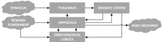
system. It is generally recognized that the hypothalamus, the amygdala, the thalamus and the hippocampus are the basic structures of this brain activity. Their loca-tion, within the human brain, can be found in several books of Neuropsychiatry such as Gloor (1997) and Lautin (2001). Beside emotions, the limbic system supports a variety of other functions such as behaviour, motivation and has a major impact on the memory formation process. It promotes the interconnection between emotional cues and reasoning leading to an internal human state of low emotional stress. This state must be attained even in the presence of distinct external or internal sensory stimuli. That is, the inputs stimuli can put the current state of the limbic system out of balance. The result is the generation of an emotional solution that will, in turn, lead to a higher degree of satisfaction. In general, those stimulus inputs are first delivered to the brain region known as the thalamus. The thalamus behaves as a sensorial switching station that gathers and pre-processes sensory data. With the exception of the olfactory sense, all other sensations are guided, by the nerves network, towards the thalamus. In turn, it forwards those different sensations directly to the amygdala or to appropriate areas of the brain such as the cerebral cortex. The cerebral cortex corresponds to the outermost layer of the brain where the most sophisticated neural processing takes place. The diagram in Figure 1 represents the signal flow within the limbic system de-parting from the thalamus structure toward the ultimate body response passing through other brain structures such as the amygdala and orbitofrontal cortex. The amygdala
Fig. 1. Amygdala based brain emotional model structure (adapted from Beheshti and Hashim (2010)).
re-sponse and promotes ways for further learning. This learn-ing and adaptation is a key element to organisms robust-ness when subjected to constantly changing environments. At the same time, robustness to condition changes is also a key feature of any engineering problem. Hence, in the last years, the brain emotional behaviour has been object of attention as a new paradigm in the control systems design field. Hence, the following section will be devoted to dissect and frame the limbic system mathematical model. It is worth to notice that the approach taken here is very different from the ones usually presented in the literature.
2.1 Brain Emotional System Mathematical Description
The robustness and efficiency exhibited by all biological systems are features that drive and inspire humans to learn from nature and try to apply this knowledge into common engineering problems. Of course, biological systems have such a high degree of complexity that, in practice, it is only possible to try to mimic their high level behaviour neglecting many of their functional details. It was in this framework that Balkenius and Mor´en (2001) presented a simplified mathematical model for the emotional learning carried out in the amygdala. This model formulation will be revisited during this section. Also, an uniform mathe-matical formulation will be laid on that spans continuous-time and discrete-continuous-time models of the limbic system.
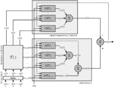
The continuous-time version This section is based on the amygdala-orbitofrontal cortex model initially proposed by Balkenius and Mor´en (2001). In it, the emotional system have the components interconnected as represented in Figure 2. A total of four main areas can be devised and coupled with the brain limbic section: the thalamus, the sensory cortex, the orbitofrontal cortex and the amygdala.
Fig. 2. Overall structure of the limbic model.
In the referred figure, it is assumed a set ofn continuous time-varying external stimuli signals denoted by i1(t)
to in(t). At this point it is assumed that these input stimuli signals are positive or zero. In addition let’s define the vector i(t) = [i1(t) · · · in(t) ]T of those external
signals. The thalamus is responsible for the generation of the internal stimulus sn+1(t) which is computed as the
maximum value of the input stimuli arrayi(t):
sn+1(t) = max{i(t)} (1)
In addition, the thalamus is responsible to forward the input stimuli to the sensory cortex. This neural structure produces the input stimuli arrays(t) = [s1(t) · · · sn(t) ]T
as a function ofi(t) according to an arbitrary
transforma-tion functransforma-tionT {·}. In Balkenius and Mor´en (2001) it was considered the identity transform. That is,
s(t) =I(n×n)·i(t) (2)
where I(n×n) is the n-dimensional identity matrix. Here,
the same transformation will be assumed. However, further research can be done to establish alternative mappings. The amygdala and the orbitofrontal cortex are the two structures where learning takes place. The amygdala in-corporates a set ofn+1 amygdala processing units (APU). It takes the values of thenstimuli signals delivered by the sensory cortex plus the one generated by the thalamus and with a reward signalr(t) associated to the stimuli vector
s(t), produces the internal outpute(t). The stimulus and
reward signals are tightly interconnected. In fact, a reward without stimulus will not lead to learning. Here, the reward signal r(t) will be assumed greater or equal to zero. The signale(t) is obtained by the following:
e(t) = n+1 X
j=1
aj(t) (3)
where aj(t) regards the output of the jth APU element at time instantt. This processing element has a structure that can be represented according to the block diagram of Figure 3. The output of each APU is computed as an weighted version of the referred excitation signals. The weighting factor, associated to the amygdala cluster j, is a positive time-varying coefficient, denoted hereby as vj(t). The APU comprises three inputs and one output. The internal stimulus signalsj(t), the reward signal r(t) associated to it and e∗(t) which concerns what can be understood as the partial amygdala output. This partial output is computed by neglecting the impact of the thala-mus stimulus in the generated signal. That is,
e∗(t) = n
X
j=1
aj(t) (4)
whereaj(t) is the output ofjthAPU at time instantt. In
Fig. 3. Diagram of the continuous-time APU element.
the block diagram of Figure 3, the triangle shape element is a gain whose value is, at time instantt and for the input stimulus j, equal to vj(t). Hence, output signal aj(t) is equal to the product ofsj(t) byvj(t). That is,
aj(t) =sj(t)·vj(t) (5) This gain value is time dependent and changes according to a learning rule represented by the dashed lines blocks and signals. One shall define ann+ 1 dimensional vector
v(k) whose elements are, besides the nweighting factors
associated to the first n amygdala clusters, the entry vn+1(t) that represents the coefficient associated to signal
sn+1(t). Here, v(t) = [v1(t) · · · vn(t)vn+1(t) ]
T
. Then, the signals generated by the amygdala can be gathered in a vectora(t) = [a1(t) · · · an(t) an+1(t) ]T obtained by,
where V(t) is a diagonal matrix whose elements are the
ones of vectorv(t). That is,
V(t) = diag{v(t)} (7)
and s∗(t) =
sT(t) sn+1(t)T is the vector obtained by
adding the element sn+1(t) to the end of vector s(t).
The model output signal u(t) depends on the difference between the amygdala output signal e(t) and the or-bitofrontal cortex output signal f(t). The orbitofrontal cortex output is obtained by summing the contributions of all the orbitofrontal processing units (OPU) whose structure is presented at Figure 4. The inputs to each of
Fig. 4. The continuous-time OPU element.
thenOPU are delivered only by the sensor cortex block. The output of a genericjthOPU is computed by,
oj(t) =sj(t)·wj(t) (8) where wi(t) is the weight associated to the ith OPU for i = 1,· · · , n. Assuming o(t) = [o1(t) · · · on(t) ]T as the
OPU output vector then,
o(t) =W(t)·s(t) (9)
where,
W(t) = diag{w(t)} (10)
withw(t) = [w1(t) · · · wn(t) ]T. The output signal of the
amygdala-orbitofrontal cortex model, at time instant t, will be denoted byu(t) and computed according to:
u(t) =1∗·a(t)−1·o(t) (11)
where 1∗ and 1 are 1×n+ 1 and 1×n unity vectors respectively. The weight update law for the OPU units is derived in the sense that the model output will follow the excitation signal when there is some reward for doing it. Hence, it will seek to minimize the following cost function,
Jv(t),w(t)=
n+1 X
i=1
vi(t)·si(t)− n
X
i=1
wi(t)·si(t)−r(t)
!2 (12)
The starting point is the conventional gradient descent algorithm whose continuous time version is given by:
∂wj(t) ∂t =−η
∂J(v(t),w(t))
∂wj(t) (13) where η > 0 is the learning coefficient. Applying this formulation, by considering the cost function expressed by (12), the following weight update rule is obtained:
∂wj(t) ∂t =β·
u(t)−r(t)·sj(t) (14)
whereβ= 2·η is the positive leaning rate coefficient. This weight update rule can be observed in the dashed line of Figure 4. For the APU units, the weights are driven toward a set of values that lead to the minimization between the reward signal r(t) and the partial amygdala signal e∗(t). This can be understood as the amygdala role to seek for
constant reward. In this framework, the cost function to be minimized has the following formulation:
J(v(t),w(t)) =r(t)−
n
X
i=1
si(t)·vi(t)2 (15)
Applying the gradient descent formulation leads to: ∂vj(t)
∂t =α·
r(t)−e∗(t)·sj(t) (16)
where α >0 is the learning rate. Notice that the weight update law for the APU is more elaborated than the above equation since it is expected that the amygdala learning weights never decrease. Hence the right member of the above expression cannot be negative. This leads to the following non-linear differential equation:
∂vj(t)
∂t =α·max
r(t)−e∗(t),0·sj(t) (17)
The APU weight update dynamics is also made evident in the dashed line blocks of Figure 3. A final remark regarding the learning ratesαandβ. Usually their initial choice are positive numbers less than one. Moreover, in the literature, the value of αis assumed to be higher than the one of β (Mor´en, 2002; Garmsiri and Sepehri, 2014). The reasoning behind this difference can be tracked down to the fact that the former contributes to the excitation and the latter to the output inhibition (Garmsiri and Sepehri, 2014).
The discrete-time version In this section it will be assumed that the stimuli signals are of discrete-time nature and defined at multiple integer time instants with period Ts. Hence the input vector is now defined as i(k) =
[i1(k) · · · in(k) ]T wherekrepresents the integer index of
the current sample and the input stimuli array iss(k) =
[s1(k)· · · sn(k) ]T. The model output is described by:
u(k) = n+1 X
j=1
aj(k)− n
X
j=1
oj(k) (18)
for,
aj(k) =sj(k)·vj(k) (19) and,
oj(k) =sj(k)·wj(k) (20) The learning law is obtained by assuming a first order approximation to the derivative operation. Using Euler forward approach, equations (14) and (17) are rewritten:
wj(k+ 1)−wj(k)
Ts =β·sj(k)·
u(k)−r(k) (21)
vj(k+ 1)−vj(k)
Ts =α·sj(k)·max
r(k)−e∗(k),0 (22)
leading to the following difference equations:
wj(k+ 1) =wj(k) + ¯β·sj(k)·u(k)−r(k) (23a)
vj(k+ 1) =vj(k) + ¯α·sj(k)·maxr(k)−e∗(k),0 (23b) where the amygdala and orbitofrontal constants are now ¯
α=Ts·αand ¯β=Ts·β and maxr(k)−e∗(k),0denotes the piecewise multivariate function:
r(k)−e∗(k) ifr(k)> e∗(k)
0 otherwise (24)
Fig. 5. The discrete-time version of the APU.
Fig. 6. The discrete-time version of the OPU.
factor is modified by a discrete-time filter with a pole at z = 1. Here, since time-domain signals are present, the backward shift operator q−1 is used instead of the
filter transfer function in theZ-domain. The filter input is excited by a piecewise linear function whose value is equal to the product of the stimulus signalsj(k) byr(k)−e∗(k) ifr(k)≥e∗(k) or 0 otherwise. Additional modification to this filter was proposed by Lotfi and Akbarzdeh (2012) where a γfactor was introduced that can modify the pole location. The intuition behind this introduction is to add a decay rate that can be used to model the brain forgetting tendency along time. A more elaborated leaning rule, for the orbitofrontal cortex, was proposed by Mor´en (2002).
2.2 The BEL based intelligent controller
A control system strategy, based on brain emotional learn-ing, was proposed by Caro Lucas in the early 2000s (Lucas et al., 2004). The limbic model used was based on the neural link, between the amygdala and the orbitofrontal cortex, proposed by Balkenius and Mor´en (2001) and de-scribed in the previous sections. This control paradigm is commonly designated by BELBIC which stands for brain emotional learning based intelligent control. The reasoning behind the integration of the limbic model into a closed loop control system can be tracked down to the seemingly robust way that the brain performs decision making. Actually, control has all to do with decision making: the controller goal is to devise the best input actions based on the incoming information according to the system states. These actions can be taken considering the past, the present or even forecasts on the future system states. Hence the controller produces a mapping between its input signals and the output control signals by means of an arbitrary decision function which can be described by means of differential equations, as in PID controllers, or by an inference mechanism such as in Fuzzy or neuro-Fuzzy control. Alternatively it can be based on the result of the optimization of a cost function such as linear quadratic regulators (LQR) or model predictive control (MPC). In the BELBIC control system architecture this input-to-output transformation is imposed by means of the limbic system model. In this case, both the external stimuli and reward signals are generated in such a way as to produce a closed loop system response according to some target characteristics. In addition, due to the recursive nature of the weights update law, this controller is able to gradually learn how to handle changes in the system dynamics. A key point in BELBIC is the external stimulus and reward
signals definition. Notice that there are not universal rules to carry out this task. This choice is flexible and must be custom defined according to the end application. Different ways to define the emotional signals can be found in the literature (Rouhani et al., 2007; Rahman et al., 2008; Nahian et al., 2014; C´esar et al., 2017). For example in Lucas et al. (2004) the reward signal r(t) is obtained as a weighted sum of the error signal and the control effort and the external stimulus signali(t) is defined as a linear combination of the system output and its first derivative.
3. THE BEL SIMULINKR
TOOLBOX
A more intuitive way to use the BEL paradigm, within a computer environment, is by means of a graphical user interface in the form of block diagram manipulations. In order to do that, a SimulinkR
toolbox was developed and made accessible through the MathWorksTM file exchange
website1. This section is devoted to describe this toolbox
how to use the main BEL blocks in a simple control system application. The idea to develop a brain emotional learning SimulinkR
toolbox is not new and has already been attempted by Mehrabian and Lucas (2006). However, there are two issues with their approach. First, it is not a toolbox but a BELBIC model for a particular problem. This approach do not provide the necessary plasticity for the user to build its own model. Second, and after an exhaustive web search, a copy of the above referred SimulinkR
file was not found.
The BELBIC toolbox file package contains an installa-tion funcinstalla-tion that the user must execute from within the MatlabR
command line environment. This can be easily done by writing >>installme at the command
prompt. The installation operation will require the user to select the BELBICtoolbox.slx and, after that, the
MatlabR
program will be automatically restarted. After the installation process, the user can navigate through the SimulinkR
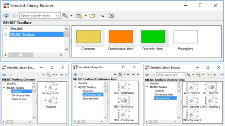
newly installed toolbox. This toolbox is di-vided into four different axis as can be seen in Figure 7. In the common section the user can find some BEL primitive functions such as the sensory cortex and the thalamus. Those objects are common to both the continuous-time and discrete-time BEL formulation. In the continuous-time
Fig. 7. The BELBIC SimulinkR
toolbox structure.
library the user may find the APU and OPU basic elements
1 http://www.mathworks.com/matlabcentral/fileexchange/
and the BEL system. All these elements have their own mask which is used to tune them by setting appropri-ate learning coefficients values and initial conditions. The same can be said about the discrete-time version. However, in this case, all the elements require the definition of a sampling period. The fourth sub-library includes a set of explanatory examples on how to fully unleash the power of the presented models. Besides the simplest ones, some more advanced control based cases are provided. Namely the control of a non-linear continuous stirred tank reactor (CSTR) as the one presented in Mehrabian and Lucas (2006) (see Figure 8). Details on both the model and BEL controller parameterization can be found in the toolbox.
Fig. 8. Non-linear CSTR control using BELBIC.
4. CONCLUSIONS
This work presented a new SimulinkR
toolbox for brain emotional learning. This library is made publicly acces-sible through the MathWorksTM file repository web site.
By providing this set of primitives, the authors believe that the researchers in this field can easily test their control problem using the BELBIC paradigm and thus contribute to disseminate the BELBIC strategy. More-over this article also describes, in the same framework, both the continuous-time and discrete-time mathematical formulation of BEL model. This can also promote the unification of the model description that, until now, it is fairly scattered along several publications and mathemat-ically inconsistent. Although, this toolbox is by no means closed. Further additions will be provided to extend its capabilities, for example by adding auto-tuning strategies.
REFERENCES
Balkenius, C. and Mor´en, J. (2001). A computational model of emotional learning in the amygdala. Cyber-netics and Systems, 32(6), 611–636.
Beheshti, Z. and Hashim, S.Z.M. (2010). A review of emo-tional learning and it’s utilization in control engineering.
Int. J. Advance. Soft Comput., 2(2).
C´esar, M.B., Gon¸calves, J., Coelho, J., and Barros, R.C. (2017). Brain emotional learning based control of a SDOF structural system with a MR damper. In CON-TROLO 2016, 547–557. Springer International Publish-ing.
Dorrah, H.T., El-Garhy, A.M., and El-Shimy, M.E. (2011). PSO-BELBIC scheme for two-coupled distillation col-umn process. Journal of Advanced Research, 2, 73–83. Fard, F.T.P., Shahgholian, G., Rajabi, A., and
Habibol-lahi, M.R. (2010). Brain emotional learning based in-telligent controller for permanent magnet synchronous motor. IPEC2010, IEEE, 989–993.
Garmsiri, N. and Sepehri, N. (2014). Emotional learning based position control of pneumatic actuators. Intelli-gent Automation & Soft Computing, 20(3), 433–450. Gloor, P. (1997). The Temporal Lobe and Limbic System.
Oxford University Press.
Huang, G., Zhen, Z., and Wang, D. (2008). Brain emo-tional learning based intelligent controller for nonlinear system.2nd Int. Symp. on Int. Inf. Tech. App., 660–663. Jafari, E., Marjanian, A., Solaymani, S., and Shahgholian, G. (2013). Designing an emotional intelligent controller for IPFC to improve the transient stability based on energy function. J. of Elec. Eng. and Tech., 478–489. Khorashadizadeh, S. and Mahdian, M. (2016). Voltage
tracking control of DC-DC boost converter using brain emotional learning. In4th International Conference on Control, Instrumentation, and Automation, 268–272. Lautin, A.L. (2001). The Limbic Brain. Springer US. Lotfi, E. and Akbarzdeh, M. (2012). Supervided brain
emotional learning. In WCCI 2012 IEEE World Congress on Computational Intelligence.
Lucas, C., Shahmirzadi, D., and Sheikholeslami, N. (2004). Introducing BELBIC: Brain emotional learning based intelligent controller. InIntelligent Automation and Soft Computing, volume 10, 11–22.
Mehrabian, A.R. and Lucas, C. (2006). A toolbox for brain emotional learning based intelligent controller. InIEEE Int. Conf. on Eng. of Intelligent Systems, 1–5.
Mohammed, M. and Bijoy, K.E. (2011). Implementation of an intelligent system for estimation of fundamen-tal frequency of speech. In IEEE (ed.), 3rd Interna-tional Congress on Ultra Modern Telecommunications and Control Systems and Workshops (ICUMT), 1–5. Mor´en, J. (2002).Emotion and Learning - a computational
model of the amygdala. Ph.D. thesis, Lund University. Nahian, S.A., Truong, D.Q., and Ahn, K.K. (2014). A
self-tuning brain emotional learning–based intelligent controller for trajectory tracking of electrohydraulic actuator. Journal of Systems and Control Engineering, 228, 461–475.
Purves, D., Augustine, G.J., Fitzpatrick, D., Hall, W.C., LaMantia, A.S., and White, L.E. (2011). Neuroscience. Sinauer Associates, Inc.; 5 edition (November 2011). Rahman, M.A., Milasi, R.M., Lucas, C., Araabi, B.N.,
and Radwan, T.S. (2008). Implementation of emotional controller for interior permanent-magnet synchronous motor drive. IEEE Transactions on Industry Applica-tions, 44(5), 1466–1476.
Rouhani, H., Jalili, M., Araabi, B.N., Eppler, W., and Lucas, C. (2007). Brain emotional learning based intel-ligent controller applied to neurofuzzy model of micro-heat exchanger. Expert Systems with Applications, 32(3), 911 – 918.
Sadeghieh, A., Roshanian, J., and Najafi, F. (2012). Im-plementation of an intelligent adaptive controller for an electrohydraulic servo system based on a brain mech-anism of emotional learning. International Journal of Advanced Robotic Systems, 9(84), 1–12.
Sarpeshkar, R. (2009). Neuromorphic and biomorphic engineering systems. McGraw-Hill Yearbook of Science and Technology 2009. McGraw-Hill.