Abstract
In order to contribute for enriching studies in the tourism field, it was intended with this research paper performing the comparison between the model based on linear regression and the model based on artificial neural networks and analyses of the performance of those models. Additionally, the usefulness of the time series that measures the number of hours of Sunshine should be confirmed. We used for this purpose the monthly series that measures the demand for tourism: “Monthly Nights in Hotels in the Northern Region of Portugal”, recorded in the period from January 1990 to December 2009.
A linear regression model based on the first differences was developed producing none statistical infractions. A previously developed ANN based model was applied for the new period of time under comparison. Both models have the sunshine time series in their entrance.
Both methodologies proved to achieve similarly good results in getting the seasonality of the time series, because the correlation coefficient was at the level of 0.99. Also both models could predict with high quality the
magnitude of the time series because the mean absolute percentage error was 4.1% and 3.5% for the linear model and for the ANN based model, respectively.
Keywords: Forecasting; Tourism Demand;
General Linear Model; Artificial Neural Networks.
Introduction
Tourism has been seen as a strategic sector in the future, for the Portuguese economy, and should influence all decision makers in this subject area to take policies that ensure their profitability and sustainability (Dolgnar & Costa, 2010).
In this sense, tourism is a truly strategic interest for the Portuguese economy because of their ability to create wealth and employment. This is a sector that showed clear competitive advantages as with few other (Ministério da Economia e da Inovação, 2006).
According to the World Tourism Organization (WTO), Portugal will reach 18.3 million foreign visitors in 2020. Tourism is at present one of the most important activities.
A comparison of linear and non linear models to forecast
the tourism demand in the North of Portugal
Natália dos Santos*, Paula Fernandes**,
João Paulo Teixeira***
* Instituto Politécnico de Bragança. Email:nspink@hotmail.com;
** Instituto Politécnico de Bragança; NECEResearch Unit in Business Sciences (Universidade da Beira Inteira).Email: pof@ipb.pt
Apart from its impact on the balance of payments and GDP, and its role on employment generation, investment and revenue, it is also recognized as the “engine” for development and other economic activities (WTO, 2011).
Similarly to Portugal also the Northern region of Portugal is ruled to be a very different region that offers an interesting alternative to the so called ‘mass tourism’, focusing on the provision of a wide variety of tourism products that range from the beach, the mountains, the thermal/health spas not forgetting the rural tourism, which had a significant increase in recent years (Fernandes, 2005).
In this respect, and given the substantial growth of this sector in the North of Portugal, it will be at all useful the development of models that could be used to make reliable forecasts of tourism demand, as it assumes an important role in the process of planning and decision-making both within the public and the private sector. At present, in the field of forecasting, is available a large variety of techniques and models that are emerging to meet the most varied situations, with different characteristics and methodologies, that range from the simple to more complex approaches (Thawornwong & Enke, 2004; Fernandes, 2005; Yu & Schwartz, 2006).
Therefore, the purpose of this paper concerns the description and comparison of two developed models, the univariate linear regression model based on the method of ordinary least squares and the other model is based on the methodology of artificial neural networks (ANN), which takes advantage of its ability to model nonlinear problems. Although, as it is intended to model and forecast the tourism demand in the North of Portugal, using econometric models, it will be used the time series of tourism “Monthly Nights in Hotels in the Northern Region of Portugal”, registered between January 1990 and December 2009.
In order to better explain this variable it will be used additionally, as an independent variable, the “Sunshine”, that is the monthly number of hours with sun. This variable already proved its interest in this type of problems in previous studies of Teixeira and Fernandes (2011).
This paper is structured as follows: after this section it will be presented a section explaining the two methodologies used in the modelling of the series under study. The following section is the presentation of time series “Monthly Nights in Hotels in the Northern Region of Portugal” and “Monthly number of hours with Sunshine”. Then follows the description of the practical implementation of the linear regression model and ANN model, defining its variables and procedures associated with the use of these methodologies. In the end of the section it is also presented the estimates of tourism demand for the year 2010 and analyses the performance of models. Finally, we will present some reflections about the study.
1. Overview of Used Methodologies
1.1. The General Linear Model
According to several authors [e.g. Oliveira
et al. (1997), Chaves (2000), Johnston & Dinardo (2000), Maroco (2003), Pestana & Gageiro (2008), Zhihua & Qihua (2009), etc] the General Linear Model (GLM) provides a general framework for a large set of models whose common goal is to explain or predict a quantitative dependent variable by a set of independent variables which can be categorical of quantitative, and encompasses techniques
such as Student’s t test, simple and multiple
linear regression, analysis of variance, and covariance analysis. In this research paper we will use the simple linear regression based on
the method of Ordinary Least Squares (OLS) to
estimate the model because it minimizes the
For the GLM, the values of the dependent variable are obtained as a linear combination of the values of the independent variables.
The vector for the coefficients of the linear
combination are stored in a K by 1 vector
denoted B. In general, the values of Y cannot
be perfectly obtained by a linear combination
of the columns of X and the difference between
the actual and the predicted values are called the prediction error. Formally the GLM is stated as (Gunst & Mason, 1980):
Y
=
XB
+
U
[1]
The predicted values are stored in an I by 1
vector and the equation can be rewritten as:
with
Y
= +
Y
U
Y
=
XB
[2]
Putting together Equations 1 and 2 shows that:
U
= −
Y
Y
[3]
According to the above explained the simple linear regression model is given by the following expression (Pestana & Gageiro, 2008):
0
t t t
Y
= +
a
b X
+
u
[4]
It should be remember that the quantitative models always rest on assumptions about the way the world works, and regression models are no exception. Therefore, in order to work with this model we need to make some assumptions about the behaviour of the error term. So, there are four major assumptions which justify the use of linear regression
models for purposes of prediction (Glass & Hopkins, 1996; Zhihua & Qihua, 2009):
(i) linearity of the relationship between dependent and independent variables; (ii) independence of the errors (no serial
correlation);
(iii) homoscedasticity (constant variance) of the errors;
(a) versus time;
(b) versus the predictions (or versus any independent variable);
(iv) normality of the error distribution. If any of these assumptions is violated (i.e., if there is nonlinearity, serial correlation, heteroscedasticity, and/or non-normality), then the forecasts, confidence intervals, and economic insights yielded by a regression model may be (at best) inefficient or (at worst) seriously biased or misleading.
1.2. Artificial Neural Networks Approach The Artificial Neural Networks models are frequently found within the broad field of knowledge related to artificial intelligence. They are based on mathematical models with an architecture that was inspired in the human brain. A neural network is composed by a set of interconnected artificial neurons, nodes, perceptrons or a group of processing units, which process and transmit information through activation functions. The connections between processing units are known as synapses. The activations functions most frequently used are the linear and the sigmoidal functions - the logistic and hyperbolic tangent functions (Fernandes, 2005). It should also be mentioned that the neurons of a network are structured in distinct layers (better known as the input layer, the intermediate or hidden layer and the output layer), with the ones most commonly used for the forecasting of time series being the multi-layers or MLP1 (Bishop, 1995), so that a neuron
from one layer is connected to the neurons of the next layer to which it can send information. Depending on the way in which they are linked between the different layers, networks can
be classified as either feedback networks2 or
feedforward networks3.
The specification of the neural network also includes an error function and an algorithm to determine the value of the parameters associated to the synapses that minimise the error function. In this way, there are two central concepts: the physical part of the network, or, in other words, its architecture, and the algorithmic procedure that determines its functioning, or, in other words, the way in which the network changes according to the data provided by the environment (Haykin, 1999).
It is also important to mention that for the ANN to learn with experience they have to be submitted to a process known as training, for which there are different training algorithms. One of the most frequently used algorithms in the forecasting of time series is the backpropagation4 algorithm or its variants,
which are distributed into two classes: (i) supervised and (ii) unsupervised (Haykin, 1999).
In brief, a value produced by a feedforward network, with one hidden layer and with a linear activation function in the output layer, can be expressed as follows (Fernandes & Teixeira, 2007):
2 The connections allow information to return to places through which it has already passed and also allow
for (lateral) interlayer connections (Fernandes, 2005). 3 Information flows in one direction from one layer
to another, from the input layer to the hidden layer and then
to the output layer (Fernandes, 2005).
4 This algorithm seeks the minimum error function in the demand space of the weights of the connections between the neurones, being based on gradient descent methods. The combination of weights that minimises the error function is considered to be the solution for the learning problem. The description of the algorithm can be analysed in
Rumelhart and McClelland (1986) and Haykin (1999).
2,1 1,
1 1
n m
t j ij t i j
j i
Y
b
α
f
β
y
−b
= =
=
+
+
∑
∑
[5] where,
m
, number of nodes in the input layer;n
, number of nodes in the hidden layer;f
, sigmoidal activation function;{
α
j,
j
=
0,1,
,
n
}
, vector of weights that connects the nodes of the hidden layer to those of the output layer;{
β
ij,
i
=
0,1,
, ;
m j
=
1, 2,
,
n
}
, weights that connect the nodes of the input layer to those of the hidden layer;2,1
b
andb
1,j, indicate the weights of the independent terms (bias) associated with each node of the output layer and the hidden layer, respectively. The equation also indicates the use of a linear activation function in the output layer.2. Presentation and Analysis of the Time Series Behaviour
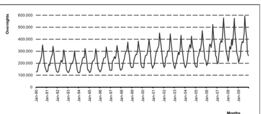
The time series Monthly Nights in Hotels in the Northern Region of Portugal is considered a significant indicator of tourist activity, since it provides information about the number of visitors that have taken advantage of tourist facilities, in this case in the North Region of Portugal.
and Monthly Number Hours of Sunshine [HS] (Figure 2). The data observed cover the period between January 1990 and December 2009, corresponding to 240 monthly observations over the 20-year period. The values for the RN series were provided by the Portuguese National Statistical Office (INE) and the HS independent series were provided by Portuguese Institute of Meteorology, and was measured in the meteorological station in the city of Porto. Since this city is the larger city in the region, and the city where the airport is located in a relatively small region, it can be considered that the Sunshine in this city is a flag for the all region.
Analysing the behaviour of the series it can be verified that there is seasonality (higher values during the summer months and lower values in winter) (Figure 1). It is also clear that there is a progressive increase over the period in question. An increase from 1998 to 2001 is also apparent, and then there is a slight decrease until 2004, and then a significant growth from 2005 to 2009. The trend is a result of economic growth and investment in the tourism sector, which have occurred in northern Portugal in recent years. However, this trend is not apparently linear. This increase may be the result of investments made in marketing variables that promoted the region both nationally and internationally.
0 100.000 200.000 300.000 400.000 500.000 600.000 Ja n -90 Ja n -91 Ja n -92 Ja n -93 Ja n -94 Ja n -95 Ja n -96 Ja n -97 Ja n -98 Ja n -99 Ja n -00 Ja n -01 Ja n -02 Ja n -03 Ja n -04 Ja n -05 Ja n -06 Ja n -07 Ja n -08 Ja n -09 O v e rn ig h ts Months 0 100.000 200.000 300.000 400.000 500.000 600.000 Ja n -90 Ja n -91 Ja n -92 Ja n -93 Ja n -94 Ja n -95 Ja n -96 Ja n -97 Ja n -98 Ja n -99 Ja n -00 Ja n -01 Ja n -02 Ja n -03 Ja n -04 Ja n -05 Ja n -06 Ja n -07 Ja n -08 Ja n -09 N o . o f H o u rs o f s u n s h in e Months
Figure 1. Overnights in Northern Portugal, from 1990:01 to 2009:12.
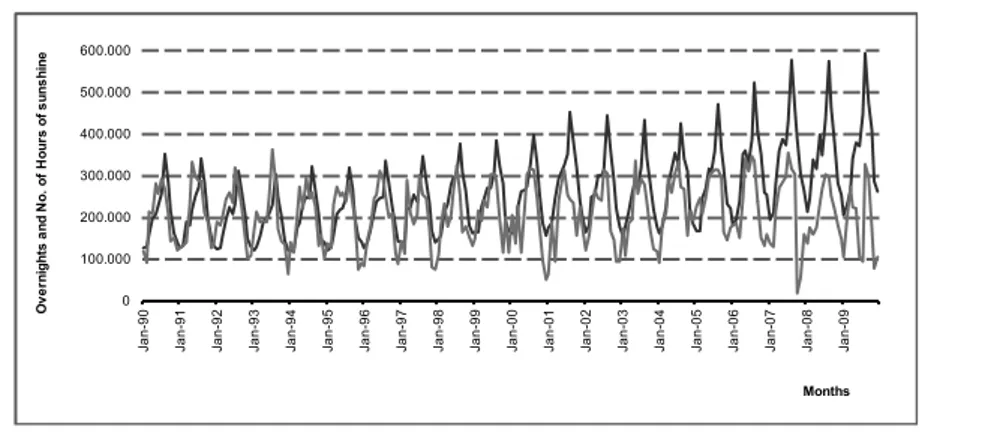
For the analysis of variable Monthly Number Hours of Sunshine showed in Figure 2 (by a question of a standardization this variable appears multiplied by 1000), can be seen that this also shows a seasonal behaviour, noting higher values the high season (between April and September) and lowest in low season (October to March). We must not forget that Portugal is known to have a Mediterranean climate and has been promoted as a country that offers sun and sea as a tourism product, which attracts thousands of visitants. In Figure 3 when overlapping the two variables the seasonal behaviour between the two series becomes clear, reflecting that the Monthly Number Hours of Sunshine can be a relevant variable that influence the tourism demand.
3. Application of Methodologies
3.1. General Linear Model
3.1.1. Simple Linear Regression Model
As mentioned in the previous section, the independent variable was the basis for model building was Hours of Sunshine in Northern region of Portugal [HS]. Thus, the mathematical model can be written as follows:
0
t t t
Overnights
= +
a
b HS
+
u
[6]
Below, Table 1 present the results obtained for the model estimated by the OLS application.
From the results obtained, it can be said that the determination coefficient is 0.32 and indicates that the Sunshine in Northern Portugal explain approximately 32% of variations taking place in Overnights in the Northern Region of Portugal.
The autonomous component and the independent variables are variables statistically significant, at a significance level of 1%, i.e. 99% of the constant’s value is a correct value (Table 1).
Regarding the analysis of the infringement of basic assumptions of the General Linear Model should be noted that:
The test the normality of the residue done by statistical test
χ
2=49,8433, with pvalue=1,50198e-011, means that this model does not follow a normal distribution, so this basic assumption of the general linear model is violated;It was observed that the average is equal
0 100.000 200.000 300.000 400.000 500.000 600.000 Ja n -90 Ja n -91 Ja n -92 Ja n -93 Ja n -94 Ja n -95 Ja n -96 Ja n -97 Ja n -98 Ja n -99 Ja n -00 Ja n -01 Ja n -02 Ja n -03 Ja n -04 Ja n -05 Ja n -06 Ja n -07 Ja n -08 Ja n -09 O v e rn ig h ts a n d N o . o f H o u rs o f s u n s h in e Months
to μ=9,7013e-013. This value is approximately zero, then the assumption of zero mean is not violated and E(μ)=0;
The homoscedasticity, constant variance of the error term, through the White test for heteroscedasticity and the test statistic TR2=17,8429 with p-value
((2)> 17,8429)=0,0001. As the p-value is less than 1%, it can be said that the model is heteroscedastic, i.e. there infringement homoscedasticity, the variance is not constant from observation to observation. Thus there is a loss of the characteristics of OLS estimators;
There were obtained the following statistic Durbin-Watson=0,550391. The statistical value of Durbin-Watson is in the positive zone autocorrelation. So it can be concluded that there is infringement of the independence of the error term and that this model suffers from autocorrelation of errors. To overcome this problem, i. e., try to correct the breach of the hypothesis of independence of the errors we applied the test of Cochrane-Orcutt, so through the estimation yielded the following statistics DurbinWatson=1,781913, and the test was inconclusive. In this regard, we applied the test Hildreth-Lu, so obtained by estimating the statistical following DurbinWatson=1,781934,
continues to find itself in the test region inconclusive. Finally, we applied the test Prais-Winsten, so obtained by estimating the statistical following Durbin-Watson=1,780265, continues to find itself in the test region inconclusive.
This model suffers autocorrelation of errors, i. e. the errors are not independent of each other with the result that the least squares estimators are not estimators with minimum variance, i. e., are not efficient while remaining non-biased, the error term does not follow a normal distribution and the variance is not constant observation to observation. Thus there is a loss of the characteristics of the OLS estimators. Once there was a violation of these assumptions it was necessary to transform the model. Therefore, the following will be described by applying the General Linear Model First Differences.
3.1.2. Model of First Differences
Formally, the General Linear Model First
Differences (MFD) and for the issue under study the model is stated as (Fernandes,
2005):
In this regard the First Differences Model represents the relationships of a particular
Table 1. Performance Measures of the Estimated Model (GLM).
Coefficient Standard Error t-ratio p-value
Constant 107414 15010,3 7,1560 <0,001
variable at a moment related with variables associated in the moments before.
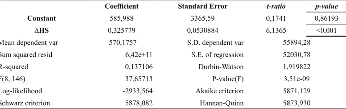
According with the results obtained (Table 2), it can be said that the determination coefficient is 0,137 and indicates that the Sunshine in Northern Portugal explain approximately 14% of variations taking place in Overnights in the Northern Region of Portugal. The variable Sunshine continues being statistically significant at a significance level of 1%, i. e., 99% of the values are correct.
Concerning the analysis of the infringement of basic assumptions of the First Differences Model, it should be noted that (Table 2):
The test of normality made by the residue of the test statistic
χ
2=6,22889, with a pvalue=0,0444032, which means that it follows a normal distribution with a significance level of 1%, then this assumption is violated;The average is equal to µ=1,2368e-014. This value is approximately zero, then the assumption of zero mean is not violated E (µ) =0;
The homoscedasticity, through the White test for heteroscedasticity and the test statistic TR2=6,40133 with p-value (
χ
2(2)>6,40133)=0,040735, as p-value is more than 1%, it concludes that do not reject the hypothesis of homoscedasticity. According to the results obtained it can be concluded that
there is no infringement homoscedasticity, i. e., the variance is constant from observation to observation. There is no loss of the characteristics of estimators OLS. The estimator continue to be BLUE5;
There was obtained a Durbin-Watson=1,919822, positioning in the area of independence of errors. Thus, the model of the first differences does not violate the assumption of independence of error terms, i. e., there is no autocorrelation of errors.
According to the results and as we see no infringement of assumptions it can be said that this model can be appropriate to model the tourist demand, however there is the requirement to evaluate its performance. 3.2. Artificial Neural Network Model
The artificial neural network used to make the prediction in this study was already developed in (Teixeira & Fernandes, 2011). In the mentioned study, four ANN here used to predict the same time series used where for the year 2009. The objective consisted in find the relevance of the Sunshine variable in the prediction of overnights. The 4 ANN have in their entrance the following features:
Model A - the previous 12 month overnights. This model here used with success in several
5 Best Linear Unbiased Estimators.
0
t t t
Overnights
a
b
HS
u
∆
= + ∆
+ ∆
[7]
Where:
1
t t t
Overnights
Overnights
Overnights
−∆
=
−
[8]
1
t t t
HS
HS
HS
−∆
=
−
[9]
1
t t t
u
u
u
−studies by the authors (Fernandes, 2005; Fernandes & Teixeira, 2007);
Model B - The entrance had only two nodes for the year and the month. The importance of this model was analyzed in (Fernandes & Teixeira, 2008);
Model C - the previous 12 month overnights plus the Sunshine. This model was the same as the model A, but including the sunshine variable. The importance of the sunshine variable should arise from the comparison of the results between model A and C.
Model D - the entrance had only three nodes for the year, the month and also for the sunshine. The importance of the sunshine variable in this model should arise from the comparison of the results between model B and D.
The results are summarized in Table 3, for the test set that corresponded to the year of 2009. Mean absolute percentage error (MAPE) is defined in following Eq. 11.
The results of Table 3 shoed the importance of the Sunshine variable in the modulation of this tourism time series, because the performance of models C and D had been improved from the model A and B, respectively.
And the model C had proved to be the best ANN model tested in the study.
Table 3. Comparison of the performance of the ANN models in (Teixeira & Fernandes, 2011).
MAPE (%) Model A
Model B
Model C
Model D Test set 4,93 7,78 4,45 7,30
Therefore, the model C has selected to this study and will be detailed in next lines.
The AAN has feed-forward architecture as presented in Fig. 4. The RNi mean the
number of Overnights of the month i, the HSi
is the number of hours of Sunshine in month i, and bn,j is the bias of the node j of layer n.
The ANN contains 13 input nodes to receive the 12 previous month overnights plus the sunshine of present month. It has 6 nodes in the hidden layer and one node in the output layer. The node of the output layer gives the predicted value for the present month. Hyperbolic tangent activation function is used in the nodes of the hidden layer, and a linear activation function in the node of the output layer. The LevenbergMarquardt
Table 2. Performance Measures of the Estimated Model.
Coefficient Standard Error t-ratio p-value
Constant 585,988 3365,59 0,1741 0,86193
backpropagation algorithm (Marquardt, 1963) has used to perform the training.
The training was performed in the work developed in (Teixeira & Fernandes, 2011), and was not repeated for the new period of time. The training was performed using the data between January of 1987 and December of 2007, in a total of 240 input output pairs. The year of 2008 consisted in the set of validation. This set has used to early stop the training process in order to avoid the over-fitting.
The model has now successively used to predict the overnight for the month of the year of 2010. To predict the month of February, the previous predicted value of January was used in the entrance and the same for following months. Therefore the target values of 2010 here never seen by the model.
4. Forecasting Tourism Demand and Performance Evaluation
In this section, the results for the test group (2010 year) will be analysed, comparing the values observed with the values forecast for the time series using the two models. It should be mentioned that the forecasting for the months of the year 2010 was undertaken without using any value observed for the year in question, in both models.
The mean absolute percentage error (MAPE) was used to measure the error distance between the predicted values and the target values of the time series.
. . .
Input layer Hidden layer Output layer
RNi-1
RNi-2
RNi-3
RNi-12
HSi
RNi
b2,1
b1,1
b1,2
b1,3
b1,4
b1,5
b1,6
1
1
( 100)
N
i i
i i
T
P
MAPE
N
=T
−
=
∑
×
[11]
Where N is the length of the test set, T and P are the target and predicted values for month i.
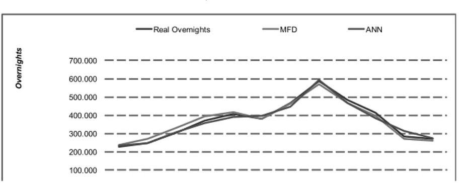
The target and predicted contours of the time series for the test set with both models are presented in Figure 5. A very close fitting was achieved with both models. The higher pick of August and the lower values of the months of January and December were very well predicted with the two models. The inflection of June was also well fitted, but slickly better with the MDF model.
The performance of the used models is presented in Table 4. The MAPE (Eq. 10) and the correlation coefficient, r, are presented for both model. The seasonality of the time series can be evaluated by the correlation coefficient and the magnitude of the predicted values are more connected with de MAPE. The r values very close to 1 prove that both models have caught the seasonal behaviour of the time series. The values between the two models are very similar. The MAPE value of 3.49% with the ANN model are even better than the one produced for the year of 2009 in (Teixeira & Fernandes, 2011), that was 4,45%. It is remarkable, because the model was trained with data until December 2007 and still producing high performance result for 2010. The MAPE of 4.14% produced with the MDF model is also a high result achieved with a model that uses only two parameters.
100.000 200.000 300.000 400.000 500.000 600.000 700.000
O
v
e
rn
ig
h
ts
Real Overnights MFD ANN
Figure 5. Comparison between Original Data and Predicted Values, from 2010:01 to 2010:12.
Table 4. Out-of-sample (test set) forecasting error measures for both models.
MDF Model ANN Model
Year r MAPE (%) r MAPE (%)
Final Conclusions
The Sunshine time series had already proved (Teixeira & Fernandes, 2011) its usefulness in the prediction of the overnight time series of tourism. In this paper the authors used this feature in the entrance of the models of two different methodologies to confirm the helpfulness of this feature and to compare the GLM models with the ANN based model.
The experiment consisted in the development of the GLM and ANN models to predict the number of overnights (RN) for the twelve months of 2010. The prediction was made without using the real values of 2010.
Concerning the modulation of the overnight time series with GLM:
• The GLM static model needs to correct the normality of the error term, the heteroscedasticity and the autocorrelation of the errors. Thus, the variance of model here not constant between observations denoting dependencies in the error term between observations. These infractions also affect the validity of the hypothesis tests and of the confidence intervals. Such as, the first differences model has applied in order to overcome the basic infractions of the static linear model. This model was denoted by the MDF model and it had presented a more satisfied statistical quality.
• The MDF model (linear model applied to the first differences) was the linear model that better model the Overnights of the North region of Portugal.
• This model did not violated the basic hypothesis, and had presented a determination coefficient and adjusted determination coefficient of approximately 14% and 13%, respectively. Therefore it was considered a good model and produced the Best Linear Unbiased
Estimators (BLUE).
The ANN based model has 13 nodes in the entrance to receive the values of the previous twelve overnight months (RNi-1 to RNi-12) and
the sunshine of present month (HSi). The
model has already used in previous studies and was trained with data until December 2007.
References
Bishop, C. (1995). Neural Networks for pattern recognition. Oxford University Press; Oxford. London.
Chaves, C. (2000). Instrumentos estatísticos de apoio à economia: conceitos básicos. Lisboa: McGraw-Hill.
Dolgnar, R. & Costa, A. (2010). Turismo, Sustentabilidade e Flexibilidade Laboral. 16º Congresso da APDR Universidade da Madeira, Funchal, pp. 801-818.
Fernandes, P. (2005). Modelación, Predicción y Análisis del Comportamiento de la Demanda Turística en la Región Norte de Portugal. Dissertação de Doutoramento, Universidad de Valladolid, Espanha. Fernandes, P. & Teixeira, J. (2007). A new
approach to modelling and forecasting monthly overnights in the Northern Region of Portugal. Proceedings of the 15th International Finance Conference, Medina, Tunísia.
Fernandes, P. O. & Teixeira, J. P. (2008).
Applying the artificial neural network
methodology to tourism time series
forecasting. In 5th International
Scientific Conference in ‘Business and
Management. Vilnius, Lithuania. ISBN 978-9955-28-267-9.
Glass, G. & Hopkins, K. (1996). Statistical Methods in Education and Psychology. (3.º Edição). Boston MA: Allyn and Bacon. Gunst, R. & Mason, L. (1980). Regression
Analysis and Its Application: A Data-Oriented Approach. Marcel Dekker, New York.
Haykin, S. (1999). Neural Networks. A comprehensive foundation. New Jersey, Prentice Hall.
IMP. (1991-2010). Instituto de Meteorologia de Portugal, IP, Lisboa, Portugal.
INE. (2010). Anuário Estatístico da Região Norte 2009. Instituto Nacional de Estatística, Lisboa, Portugal.
Johnston, J. & Dinardo, J. (2000). Métodos Econométricos. 4ª Edição, McGraw-Hill. Marquardt, D. (1963). An Algorithm for
Least-Squares Estimation of Nonlinear Parameters. Journal on Applied Mathematics, 11(2): 431-441.
Maroco, J. (2003). Análise Estatística com utilização do SPSS. Lisboa: Edições Sílabo, Lda.
Ministério da Economia e da Inovação. (2006). Plano Estratégico Nacional do Turismo - Para o desenvolvimento do Turismo em Portugal. Lisboa.
Oliveira, M., Aguiar, A., Carvalho, A., Martins, F., Mendes, V. & Portugal, P. (1997).
Econometria Exercícios. Lisboa:
McGraw-Hill.
WTO. (2011). United Nations World Tourism Organization, Tourism Market Trends. Publicação [online]. UNWTO, 2006. Disponível em URL: http://www.unwto. org 02/2011.
Pestana, M. & Gageiro, J. (2008). Análise de Dados para Ciências Sociais A complementaridade do SPSS. (5.º Edição); Lisboa: Edições Sílabo, Lda. Rumelhart, D. & McClelland, J. (1986). Parallel
Teixeira, J. P. & Fernandes, P. O. (2011). A Insolação como Parâmetro de entrada em modelo baseado em Redes Neuronais para previsão de série temporal do Turismo. Actas do VI Congresso LusoMoçambicano de Engenharia; Maputo, Moçambique. ISBN: 978-972-8826-24-6.
Thawornwong, S. & Enke, D. (2004). The adaptive selection of financial and economic variables for use with artificial neural networks. Neurocomputing, 6, 205-232.
Yu, G. & Schwartz, Z. (2006). Forecasting Short Time-Series Tourism Demand with Artificial Intelligence Models. Journal of Travel Research, 45,194-203.