Fuzzy Linear Programming: Optimization of an Electric Circuit Model
A.M.A. BERTONE, R.S.M. JAFELICE and M.A. C ˆAMARA*
Received on November 19, 2016 / Accepted on June 16, 2017
ABSTRACT.A problem of a voltage division circuit is modeled in order to determine the values of the resistors centered, in a way that the impedance of the resistance voltage divider is minimal. This problem is equivalent to maximizing the admittance, associated to the resistance, which is defined as the quotient of the electric current and its voltage, measured in Siemens. Three cases are analyzed for the components of the linear programming: real numbers, fuzzy numbers of type-1, and fuzzy sets of type-2. The first case is considered in order to validate the other two cases. The optimal solution in the fuzzy linear programming of type-1 is obtained through a linear defuzzification function, defined in the trapezoidal fuzzy numbers sub-space of fuzzy numbers vector sub-space, which allows to solve the corresponding linear programming problem with real components. A study upon the parameter for linear defuzzification is accomplished to determine the best representative of the family of parameters. Theα−levels representation theorem is the method to obtain the optimal solution of type-2. For eachα−level is solved a fuzzy linear programming problem of type-1, using the previous methodology. Numerical simulations illustrate the results in the three cases.
Keywords:electrical circuit model, linear programming, fuzzy linear programming, fuzzy sets of type-1, fuzzy sets of type-2.
1 INTRODUCTION
Being one of the most important field of Operational Research, Linear Programming (LP) con-cerns to models that optimize linear objective function and constraints on the decision variables. Efficient algorithms has been developed for LP, among which we point out the interior point [12], and the simplex algorithm [3].
One of the important issues of LP is that the modeling needs well-defined and precise data, which in general involves high information costs. Indeed, this is a task almost impossible to accomplish in many cases, due to risk or uncertainty in some data [9]. This problem of the classical LP can be contoured with the use of fuzzy numbers. Fuzzy Linear Programming (FLP) explains the mathematical model in a more realistic way [11]. Basically, considering some of the components
*Corresponding author: Marcos Antˆonio da Cˆamara – E-mail: camara@ufu.br
of a LP as fuzzy numbers, a constraint violation is allowed, and the degree of satisfaction of a constraint is defined as the membership function of the constraint [9].
One of the basic references in the area of FLP is due to Bellman and Zadeh [2]. The type of FLP that has been considered for this research is the possibilistic programming, that recognizes uncer-tainties in the objective function coefficients, as well as in constraint coefficients. The member-ship function is used to represent the degree of satisfaction of constraints, the decision-maker’s expectations about the objective function level, and the range of uncertainty of coefficients [9].
Based in the great success of the FLP, the approach is applied to a voltage divider model. In fact, an electrical circuit has components characterized by diverse parameters, each one associated to a tolerance, given by the product manufacturer. For example, a resistance of 48 ohms can have
±10% tolerance, due to temperature, time of use, among other reasons [10]. This gradualness motivated this study to use the fuzzy linear programming approach for a problem of a voltage divider. The value given by the electric appliance manufacturer is called the centered value. The tolerances and the centered values allow better control over the limits under which the circuit keeps operating and, thereby, optimize its performance. The model use for this research was built by Salazar in [10]. The objective of this research is to study three cases for the components of the LP. The first case is for real numbers components we proposed of validating the other two results. The second case refers to trapezoidal fuzzy number of type-1 as a components of LP system. The optimal solution is obtained through a total linear order defuzzification function, defined in the trapezoidal fuzzy numbers subspace of fuzzy numbers vector space. The third case extends the second case for type-2 independent LP components. The α−levels representation theorem is the method to obtain the optimal solution of type-2. For the numerical simulation for all cases it is use the classical interior point method [12], using the linear programming algorithm linprog of the software MatlabR, and an algorithm that reproduces the representation theorem.
This work is organized into six sections. Section 1 is the introduction to this study. In Section 2 the mathematical model of the electrical circuit is explained. In Section 3 a fuzzy background for the electrical circuit is detailed. In Section 4 the fuzzy linear programming method for the model is developed. The numerical results are shown in Section 5, and conclusions are drawn in Section 6.
2 MATHEMATICAL MODEL OF THE ELECTRICAL CIRCUIT
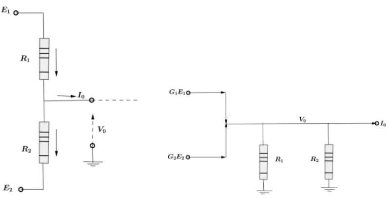
The voltage divider circuit shown in [10], illustrated in Figure 1(a), is the model to be built in this section.
In this circuit are considered two voltage generators, each producing an electromotive force,
E1 and E2, measured in volts. Suppose that E1 > E2 for the circuit shown in Figure 1(a),
the current in the direction indicated by the arrows. It is assumed that the tolerances associated with respective potential have a minimum value E−1, and maximum E1+, with respect to E1.
Analogously, there exist minimum valueE2−, and maximumE2+, with respect toE2. The goal of
(a) The circuit model of voltage divider (b) Parallel circuit model of voltage divider
Figure 1: Equivalente basic circuit of voltage divider.
the resistant voltage divider is minimal. Further, as restrictions, the output potential,V0, belongs
to the interval[V0m,V0M], where the exponentmstands for the minimum value, andM, for the maximum. The current,I0, is in the range[I0m,I0M]. The tolerances verify the inequalities
E−1 ≥V0M ≥V0m ≥E2+. (2.1)
The total impedance of the resistant voltage divider is given by the formula
R0=
R1 R2
R1+R2 ,
due to the fact that the two resistors are in parallel. In order to obtain a linear model, the variable resistors are replaced by the associated admittance, which are given by the inverse of the values
Gi = 1/Ri,i = 0,1,2. With this notation, total admittance dividerG0 = G1+G2. As a
consequence, the objective function of the problem is given by
G−0 =G−1 +G−2,
which it will be maximized. Denoting byG1andG2the centered values of the admittanceG1
andG2, respectively, then we have
G−1 =(1−ǫ1)G1andG−2 =(1−ǫ2)G2,
whereǫ1andǫ2are two known tolerances. Thus, the proposed linear programming problem is
given by
In order to express the constraints on the variablesG1andG2, we observe, based in Figure 1(b),
that
I =I1+I2+I0.
Consequently, we get
G1E1+G2E2=
V0
R1
+ V0
R2
+I0.
Hence,
G1E1+G2E2=V0
1
R1
+ 1
R2
+I0,
from where, it is obtained
G1E1+G2E2−I0=V0(G1+G2).
Therefore,
V0=
E1G1+E2G2−I0
G1+G2 .
Analyzing the behavior ofV0in relation to the variations ofG1,G2, andI0, we have:
(I) Calculating the partial derivative ofV0with respect toG1, we obtain
∂V0 ∂G1
= E1(G1+G2)−(E1G1+E2G2−I0)
(G1+G2)2
= E1G1+E1G2−E1G1−E2G2+I0
(G1+G2)2
= (E1−E2)G2+I0
(G1+G2)2
> 0,
(2.3)
due to the fact thatE1>E2. As a conclusion, we get thatV0decreases asG1decreases.
(II) Calculating the partial derivative ofV0with respect toG2, we have
∂V0 ∂G2
=(E2−E1)G1+I0
(G1+G2)2
<0, (2.4)
sinceI =I1+I2+I0so that
Thus,
∂V0 ∂G2
= (E2−E1)G1+I0
(G1+G2)2
= G1E2−G1E1+G1E1+G2E2−V0G1−V0G2
(G1+G2)2
= E2(G1+G2)−V0(G1+G2)
(G1+G2)2
= E2−V0
G1+G2 .
Since we have E1− ≥ V0M ≥ V0m ≥ E2+, then E2 < V0, therefore E2−V0 < 0. This
implies that
∂V0 ∂G2
<0,
meaning thatV0decreases asG2increases.
(III) From the fact thatG1+G2>0, we conclude ∂V0 ∂I0
= −1
G1+G2 <0
which yieldsV0decreases as I0increases.
Consequently,V0will assume its lowest value, which it is desired to be not less thanV0m, when
G1assumes its lowest value G−1. Besides, G2 assumes its highest value, G+2, and the current
obtainedI0isI0M.
Therefore, the constraintV0m≤V0is equivalent to
V0m≤E
− 1G
− 1 +E
− 2G
+ 2 −I0M
G−1 +G+2
or, alternatively,
V0m≤E
−
1(1−ǫ1)G1+E −
2(1+ǫ2)G2−I0M (1−ǫ1)G1+(1+ǫ2)G2
,
that is,
(1−ǫ1)(E−1 −V
m
0 )G1+(1+ǫ2)(E−2 −V
m
0 )G2≥I0M.
Similarly, the constraintV0≤V0M is equivalent to
(1+ǫ1)(E+1 −V0M)G1+(1−ǫ2)(E+2 −V0M)G2≤I0m.
Consequently, the mathematical model for the linear programming for the problem of the voltage divider is given by
maxH(G1,G2)= [(1−ǫ1)G1+(1−ǫ2)G2]
(1−ǫ1)(E1−−V0m)G1+(1+ǫ2)(E2−−V0m)G2≥I0M
Using the notations
ǫ=
1−ǫ1
1−ǫ2
, G=
G1 G2
, ϒ=
−I0M
I0m
, O=
0 0 , and =
(1−ǫ1)(V0m−E1−) (1+ǫ2)(V0m−E2−) (1+ǫ1)(E1+−V0M) (1−ǫ2)(E2+−V0M)
we have the PL system translate to the matrix form
maxH(G)=ǫTG G≤ϒ
G≥O.
(2.5)
3 FUZZY BACKGROUND FOR THE ELECTRIC CIRCUIT MODEL
In this section, we sumarize the relevant concepts of fuzzy sets of type-1, and fuzzy sets of type-2, which details can be found in [2, 5, 6]. Given a universe set,X, the set
A= {(x, µA(x)),x ∈X},
whereµAa function is a fuzzy set of type-1 over X, corresponding to the membership function
µA. The assembly of all fuzzy sets of type-1 is denoted byF(X). Given a numberα∈ [0,1], the
α−level of the fuzzy setAis the set defined by
[A]α = {x∈ X, µA(x)≥α}.
Considering the set
supp(A)= {x∈ X, µA(x) >0},
which is, by definition, the support of the set A, the zero level of Ais the closure of supp(A), denoted by supp(A).
Any fuzzy set can be regarded as a family of fuzzy sets. This is the essence of an identity principle known as the representation theorem. The representation theorem states that any fuzzy set Acan be decomposed into a series of itsα−level [7].
The fuzzy set of type-1, A, is called a fuzzy number when X = R, there isx ∈ X such that
µA(x) = 1, allα-levels are not empty and are closed intervals, and A has bounded support. In this study is considered the fuzzy numbers defined as singleton of type-1, given through the membership function
µr(x)=
1 ifx=r
0, ifx=r,
Another type of fuzzy number considered is the trapezoidal fuzzy number defined by the mem-bership function
µA(x)= ⎧ ⎪ ⎪ ⎪ ⎪ ⎪ ⎪ ⎪ ⎪ ⎨ ⎪ ⎪ ⎪ ⎪ ⎪ ⎪ ⎪ ⎪ ⎩
x−a
m−a, ifx∈ [a,m]
1, ifx∈ [m,n]
b−x
b−n, ifx ∈ [n,b]
0, otherwise,
denoted byA=(a,m,n,b). The interval[m,n]is known as the kernel of the trapezoidal fuzzy numberA.
A fuzzy set of type-2,A, onXis the set
A= {(x,u);µA((x,u)), (x,u)∈X× [0,1]},
whereµA: X× [0,1] → [0,1]is the associated membership of the fuzzy set A. The secondary membership function ofx′∈X is the fuzzy set of type-1 which universe is the set
Ux′ = {u∈ [0,1], µ
A(x′,u) >0}
and its membership is giving byµA(x′,u), withu ∈Ux′. Geometrically, this fuzzy set is obtained
by the vertical cut with the parallel plane to the axisupassing throughx=x′.
The so called superior primary membership function of type-1 denoted byµA(x), and the inferior primary membership function of type-1,µ
A(x),x∈ X, are defined by
µA(x)=sup{u ∈ [0,1], µA(x,u) >0}, (3.1)
µ
A(x)=inf{u ∈ [0,1], µA(x,u) >0}. (3.2) A fuzzy set of type-2 that verifiesµA((x,u))=1 for all(x,u)∈ X× [0,1]is called an interval fuzzy set of type-2. When these type of sets haveµ
A =µA(x)for allx∈ X, known as singleton of type-2.
We define the operation of addition between trapezoidal fuzzy numbers. Indeed, let Ai =
(ai,mi,ni,bi),i =1,2, two trapezoidal fuzzy numbers. By definition, we have
A1+A2=(a1+a2,m1+m2,n1+n2,b1+b2).
An external product givenα∈R+is defined by
α·A1=α(a1,m1,n1,b1)=(α·a1, α·m1, α·n1, α·b1).
In the case thatα∈R−, the definition is
With these definitions, the set of trapezoidal fuzzy numbers is a vector subspace of F(R), which we denote byT rap(R).
Several proposals for an order relation, not necessarily a total order, over the setT rap(R)can be found in the literature [1, 4, 8]. In this study, it is proposed a novel total order in a particular vector subspace ofT rap(R), composed by the fuzzy numbers
{A=(a,a,n,b), a, n, b∈R}. (3.3)
The set described in (3.3) it is denoted as T rapRight(R). It is easy to proved that the set
T rapRight(R)is, in fact, a subspace ofT rap(R).
Let A∈ T rapRight(R), the new total order relation is constructed through the so call
defuzzifi-cation function associated to the order [1], given by
gγ(A)=b+γ (n−b), γ ∈ [0,1], (3.4)
whereγis a parameter in the interval[0,1]that we defined as parameter of defuzzification ofg. Defining a equivalence relation inT rapRight(R)as
Ais equivalent toBif and only ifg(A)=g(B), for all A, B∈T r apRight(R), (3.5)
and the order relation
Ais related toBif and only ifg(A) >g(B), for allA, B∈T r apRight(R), (3.6)
it is clear that this relation is a total order (3.6) uponT rapRight(R), along with the equivalence
relation (3.5), determines a total order in this set, denoted by “ ”. The total order (3.6) is used in next section in order to transform a fuzzy linear programming in a classical one to obtain a fuzzy solution of the model (2.5).
4 FUZZY LINEAR PROGRAMMING METHODS FOR THE ELECTRICAL CIRCUIT MODEL
In this section, we consider the LP problem described in Section 2, which is given by the matrix form (2.5). The objective to use the FLP approach is to allow a constraint violation. This exten-sion of the model is made through the coefficients of the objective function, and the constraints, using fuzzy numbers for its coefficients. Therefore, we consider the elements of LP components
H,, andϒin three cases:
1. real numbers (classical LP). In order to validate the proposed methods;
2. fuzzy numbers (FLP of type-1). The coefficients ofH, and the entries ofare elements ofT rapRight(R). The vectorϒ=(I0M,I0m), whereI0M andI0m ∈R;
The first component of the vectorϒ is a fuzzy set of type-2 defined by the membership function
µI0m(x,u)= ⎧ ⎪ ⎪ ⎪ ⎨ ⎪ ⎪ ⎪ ⎩
α,ifx ∈ [I0m−δL,I0m],
ux =
x−I0m+δL(1−α)
δL(1−α)−I0m
, forα∈ [0,1],
whereI0m−δLis the minimum of level zero.
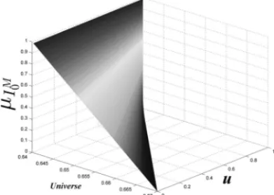
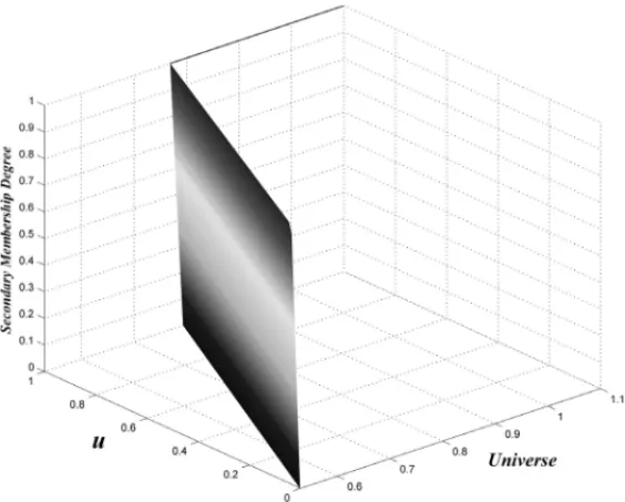
The second component of the vectorϒis a fuzzy set of type-2 defined by the membership function
µIM
0 (x,u)= ⎧ ⎪ ⎪ ⎪ ⎨ ⎪ ⎪ ⎪ ⎩
α,ifx∈ [I0M,I0M +δR],
ux =
I0M +δR(1−α)−x
I0M +δR(1−α)
, forα∈ [0,1],
whereI0M +δRis the maximum of level zero.
The graphics of these fuzzy sets of type-2 are shown in Figure 2 for the independent constraintIm
0, and in Figure 3 forI0M.
Figure 2: The fuzzy set of type-2 correspond-ing to the independent term of the second con-straint.
Figure 3: The fuzzy set of type-2 correspond-ing to the independent term of the first con-straint.
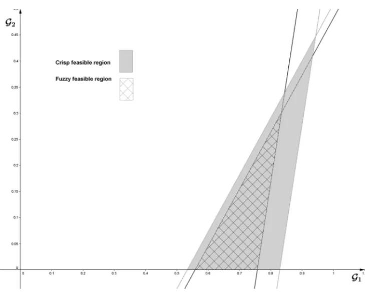
The motivation to study the third case comes again, to allow a constraint violation in terms of the interval[I0m,I0M]. Extending this interval to[I0m −δL,I0M +δR], for chosen values ofδL and
δR for which the PL has solution, induces to a feasible region, that we called the fuzzy feasible region, to be included in the crisp feasible region. Indeed, the PL constraint associated to the fuzzy feasible region is given by
(1−ǫ1)(E1−−V0m)G1+(1+ǫ2)(E2−−V0m)G2≥I0M+δR
Figure 4: The crisp and fuzzy feasible regions for the valuesδL =0.03 andδR=0.05.
which yields in the set shown in Figure 4.
The extreme values, for which the PL has solution,δLandδRare
0≤δL<0.335 and 0≤δR <0.207.
For the numerical simulations of Section 5, the values chosen areδL=0.03 andδR=0.05.
On the order hand, the resolution method applied in the case of the classical LP is the interior point [12], using the linear programming algorithm linprog of the software MatlabR.
For case 2, it is applied the defuzzification ordergγ on the fuzzy coefficients of the objective function, and the constraints, in order to calculate the optimum point through the case 1 method.
For case 3, it is defined a parametric family indexed byαof PL problems of type-1, obtained by the cuts of the vectorϒat theα−level. It is solved for eachαa PL problem of type-1, the method used in case 2. The solution is obtained by applying the representation theorem ofα−levels of the sets of type-2 [6].
5 NUMERICAL RESULTS
H(G1,G2)=0.6G1+0.9G2, =
−1.2 1.1
0.7 −0.18
and ϒ =
−0.64
0.58
,
whereǫ1 is ±40%, and ǫ2 is±10%. The optimal solution obtained is H(0.9437,0.4477) =
0.9691.
For case 2, the components considered are:
H(G1,G2)=(0.4,0.6,1,1)G1+(0.6,0.9,1,1)G2,
=
(−2,−2,−1.2,−0.8) (1,1,1.1,1.4) (0.5,0.5,0.7,0.8) (−0.2,−0.2,−0.18,−0.12)
and ϒ=
−0.64
0.58
.
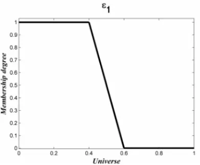
The fuzzy trapezoidal numbersǫ1andǫ2used to construct the coefficients of the objective
func-tionH, and the entries of the matrixare shown in Figure 5 and Figure 6.
Figure 5: The fuzzy trapezoidal number ǫ1
used to construct the coefficients of the objec-tive functionH.
Figure 6: The fuzzy trapezoidal number ǫ2
used to construct the coefficients of the objec-tive functionH.
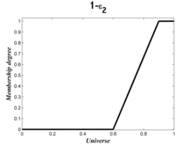
The graphics of the coefficients, 1−ǫ1and 1−ǫ2for the objective functionH, are shown in
Figure 7 and Figure 8.
The entries of the matrixare shown in Figure 9 and Figure 10 (first row), and in Figure 11 and Figure 12 (second row).
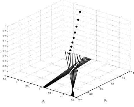
We considerγ ∈ [0.3,1]since that values lesser than 0.3 cause the linear programming to fail in encounter optimal solutions. For the valueγ =1 we havegγ(A)=n. As a consequence, the optimum point of the case 2 coincides with the case 1, and the optimum value is the minimum of level 1 of optimum fuzzy number:
H(0.9437,0.4477)=(0.5517,0.9691,1.3913,1.3913).
Figure 7: Coefficient 1−ǫ1 of the objective
functionH.
Figure 8: Coefficient 1−ǫ2of the objective
functionH.
Figure 9: Entry A11of the matrix. Figure 10: EntryA12of the matrix.
0.5 0.6
0.7 0.8
0.9 1
−1.5 −1 −0.5 0 0.5 1 1.5
0 0.1 0.2 0.3 0.4 0.5 0.6 0.7 0.8 0.9 1
H
G2 G1
Figure 13: The optimal points corresponding to different values ofγ.
For eachγ, defuzzification parameter in the interval[0.3,1], the optimum point is a fuzzy num-ber of type-1, because for each level we get an optimum point (crisp), and a corresponding trape-zoid optimal solution at this point. Thus, the optimum point has the fuzzy universe determined by the optimum level zero and level one, which in Figure 14 is represented by the black points. The membership function is the line determined by the points in space, whose first two coordi-nates are the coordicoordi-nates of the optimum point level zero, and level one. The third coordinate is zero and one, respectively.
0.87 0.88 0.89 0.9
0.91 0.92 0.93 0.94
0.15 0.2 0.25 0.3 0.35 0.4 0 0.2 0.4 0.6 0.8 1
G1 G2
Membership Degree
In Figure 15, it is shown the graph of the optimal solution of type-2 obtained from each optimum point of Figure 14, and its corresponding optimal fuzzy solution. The gradient of gray colors in both the figures are corresponding and represent the levels from 0 to 1.
Figure 15: The fuzzy solution of type-2.
It is shown in Figure 16 the optimal points, and in Figure 17 the fuzzy solution of type-2 for values ofγ in the interval[0.7,1].
6 CONCLUSION
Figure 16: The optimal points corresponding to values of γ ∈ [0.7,1], and its membership degrees.
Figure 17: The fuzzy solution of type-2 corresponding to values ofγ ∈ [0.7,1].
RESUMO. Um problema de divis˜ao de tens˜ao de um circuito ´e modelado com o objetivo
de determinar os valores centrados das resistˆencias, de maneira que a impedˆancia resistiva do divisor de tens˜ao seja m´ınima. Este problema ´e equivalente a maximizar as admitˆancias,
vol-tagem, medida em Siemens. Trˆes casos s˜ao analisados para os componentes de programac¸˜ao
linear: n´umeros reais, n´umeros fuzzy do tipo 1 e conjuntos fuzzy do tipo 2. O primeiro caso ´e considerado para a validac¸˜ao dos outros dois casos. A soluc¸˜ao ´otima na programac¸˜ao linear
fuzzy do tipo 1 ´e obtida atrav´es de uma func¸˜ao de defuzzificac¸˜ao linear, definida no subespac¸o
dos n´umeros fuzzy trapezoidais do espac¸o vetorial dos n´umeros fuzzy, o que permite resolver o correspondente problema de programac¸˜ao linear com componentes reais. Um estudo sobre
o parˆametro para a defuzzificac¸˜ao linear ´e realizado para determinar o melhor representante
da fam´ılia de parˆametros. O teorema de representac¸˜ao dosα-n´ıveis ´e o m´etodo para obter a soluc¸˜ao ´otima do tipo 2. Para cadaα-n´ıvel ´e resolvido um problema de programac¸˜ao linear
fuzzy do tipo 1 utilizando a metodologia anterior. Simulac¸ ˜oes num´ericas ilustram os
resulta-dos nos trˆes casos.
Palavras-chave:modelo de circuito el´etrico, programac¸˜ao linear, programac¸˜ao linear fuzzy,
conjuntos fuzzy do tipo 1, conjuntos fuzzy do tipo 2.
REFERENCES
[1] J.M. Adamo. Fuzzy decision trees.Fuzzy Sets and Systems,4(1980), 207–219.
[2] R.E. Bellman & L.A. Zadeh. Decision-making in a fuzzy environment. Management Science, 17(1973), 149–156.
[3] G.B. Dantzig. “Origins of the simplex method”.Technical Report SOL 87-5, Department of Opera-tions Research, Stanford University, Stanford, CA (1987).
[4] D. Dubois & H. Prade. Operations on fuzzy numbers.International Journal of Systems Science, 9(1978), 613–626.
[5] N.N. Karnik, J.M. Mendel & Q. Liang. Type-2 fuzzy logic systems.IEEE Trans. on Fuzzy Systems, 7(1999), 643–658.
[6] J.M. Mendel, M.R. Rajatia & P. Sussner. On clarifying some definitions and notations used for type-2 fuzzy sets as well as some recommended changes.Information Sciences,340–341(2016), 337–345.
[7] W. Pedrycz & F. Gomide. “An Introduction to Fuzzy Sets: Analysis and Design”. MIT Press, (1998).
[8] H. Prade, R.R. Yager & D. Dubois (Editors). “Readings in Fuzzy Sets for Intelligent Systems”. Morgan Kaufmann Publishers, (1993).
[9] N. Sahinidis. Optimization under uncertainty: state-of-the-art and opportunities.Computers and Chemical Engineering,28(2004), 971–983.
[10] J.J. Salazar Gonz´alez. Optimizaci´on matem´atica: Ejemplos y aplicaciones.Technical report Univer-sidad de La Laguna, Espa ˜na,https://imarrero.webs.ull.es/sctm03.v2/, (2003).
[11] J.L. Verdegay. “Fuzzy Mathematical Programming”. In: Fuzzy Information and Decision Processes, pp. 231–237, M.M. Gupta & E. S´anchez Editors, (1982).
![Figure 16: The optimal points corresponding to values of γ ∈ [0.7, 1], and its membership degrees.](https://thumb-eu.123doks.com/thumbv2/123dok_br/16167156.707446/15.1063.239.890.160.579/figure-optimal-points-corresponding-values-γ-membership-degrees.webp)
