Available online at www.ispacs.com/jfsva Volume 2014, Year 2014 Article ID jfsva-00196, 11 Pages
doi:10.5899/2014/jfsva-00196 Research Article
Variational Iteration Method for Solving a Fuzzy Generalized
Pantograph Equation
A. Amiri∗
Department of Mathematics, Science and Research Branch, Islamic Azad University, Tehran, Iran
Copyright 2014 c⃝A. Amiri. This is an open access article distributed under the Creative Commons Attribution License, which permits unrestricted use, distribution, and reproduction in any medium, provided the original work is properly cited.
Abstract
A numerical method for solving the fuzzy generalized pantograph equation under fuzzy initial value conditions is presented. This technique provides a sequence of functions which converges to the exact solution to the problem and is based on the use of Lagrange multipliers for identification of optimal value of a parameter in a functional. To display the validity and applicability of the numerical method two illustrative examples are presented.
Keywords:Variational iteration method; Generalized Pantograph equation; Fuzzy differential equation; Generalized Hukuhara dif-ferentiability
1 Introduction
Fuzzy differential equations are utilized for the purpose of the modelling problems in science and engineering. Most of the problems in science and engineering require the solutions of a fuzzy differential equation which are satisfied with fuzzy initial conditions, therefore a fuzzy initial value problem is occurring, and should be solved. The topic of fuzzy differential equations has been rapidly growing in recent years.
The concept of the fuzzy derivative was first introduced by Chang and Zadeh [15], it was followed up by Dubois and Prade [19]. Kaleva in [26] and [27] proposed fuzzy differential equations using H-derivative and it was developed by some other authors (see [[31], [11], [14], [13], [16], [18], [25], [7], [5], [6], [9], [21]]). The numerical methods for solving fuzzy differential equations are introduced in [1], [2], [4], [3].
The name pantograph originated from the study [30] by Ockendon and Tayler. These equations arise in industrial applications and in studies based on biology, economy, control theory and electrodynamics, among others. Properties of the analytic solution of these equations as well as numerical methods have been studied by several authors [17], [29], [20]. In [28], the authors introduced a numerical method based on the Taylor polynomials for the approximate solution of the fuzzy pantograph equation with linear functional argument.
The purpose of the present paper is to develop and apply variation iteration methods to the generalized pantograph equation with fuzzy initial conditions.
This paper is organized as follows: In Section 2, we describe the basic notations and preliminaries. In Section 3, the variational iteration method is briefly described. We define the fuzzy generalized pantograph equation under generalized Hukuhara differentiability in Section 4 and according to the type of differentiability, the solutions of the fuzzy generalized pantograph equation are investigated. Some numerical examples are given to clarify the details and efficiency of the method in Section 5. We end up with some conclusions.
2 Basic concepts
In this section, we represent some definitions and introduce the necessary notation which will be used throughout the paper.
Definition 2.1. A fuzzy number is a function such as u:Rn→[0, 1]satisfying the following properties:
(i) u is normal, i. e, ∃t0∈Rwith u(t0) =1;
(ii) u is convex fuzzy set i. e, u(λx+ (1−λ)y)≥min(u(x), u(y))∀x,y∈R, λ∈[0, 1];
(iii) u is upper semi-continuous on R;
(iv) closure of{t∈Rn|u(t)>0}is compact. ThenRF is called the space of fuzzy numbers.
For 0<α≤1 denoteu(α) =
{
t∈Rn
u(t)≥α
}
= [u(α),u(α)]. Then from(i)to(iv), it follows that theα-level set
u(α)is a closed interval for allα∈[0, 1]. For arbitraryu, v∈RF andk∈R, the addition and scalar multiplication are defined by(u+v)(α) =u(α) +v(α), (ku)(α) =k(u(α))respectively. [8]
Ifu⊕v=w, thenw⊖v=u; here,⊖is the Hukuhara difference.
Definition 2.2. [12] Given two fuzzy numbers u,v∈RF, the generalized Hukuhara difference (gH-difference for
short) is the fuzzy number w, if it exists, such that
u⊖gHv=w⇐⇒
{
(i) u=v+w,
or(ii) v=u+ (−1)w. (2.1)
It is easy to show that(i)and(ii)are both valid if and only if w is a crisp number.
In terms ofα-cuts we have[u⊖gHν]α= [min{u(α)−v(α), u(α)−v(α)}, max{u(α)−v(α), u(α)−v(α)}]and if the H-difference exists, then u⊖v=u⊖gHv; the conditions for the existence of w=u⊖gHv∈RF are
case(i)
{
w(α) =u(α)−v(α)and w(α) =u(α)−v(α)
with w(α)increasing,w(α)decreasing, w(α)≤w(α), ∀α∈[0,1], (2.2)
case(ii)
{
w(α) =u(α)−v(α)and w(α) =u(α)−v(α)
with w(α)increasing,w(α)decreasing, w(α)≤w(α), ∀α∈[0,1], (2.3)
Letα-level representation of fuzzy-valued function f :[a, b]→RF is expressed by f(t;α) = [f(t;α), f(t;α)],
t∈[a,b], for eachα∈[0, 1].
Definition 2.3. [12]. Let t0∈]a,b[and h be such that t0+h∈]a,b[, then the gH-derivative of a function f: ]a,b[→
RF at t0is defined as
fgH′ (t0) =lim
h→0
f(t0+h)⊖gH f(t0)
h . (2.4)
If fgH′ (t0)∈RF satisfying (2.4) exists, we say that f is generalized Hukuhara differentiable (gH-differentiable for
short) at t0.
Theorem 2.1. [12] Let f :]a, b[→RF be such that f(t;α) = [f(t;α), f(t;α)]. Suppose that the functions f(t;α)
and f(t;α)are real-valued functions, differentiable w.r.t. t , uniformly w.r.t. α ∈[0, 1]. Then the function f(t)is gH-differentiable at a fixed t∈]a, b[if and only if one of the following two cases holds:
(b) f′(t;α)is decreasing, f′(t;α)is increasing as functions ofα, and f′(1;α)≤f′(1;α). also,∀α∈[0, 1]we have
fgH′ (t;α) = [min{f′(t;α), f′(t;α)}, max{f′(t;α), f′(t;α)}]. (2.5) Definition 2.4. [12] Let f: [a, b]→ RF and t0∈]a,b[with fα(t;α)and fα(t;α)both differentiable at t0. We say
that :
• f is (i)-gH-differentiable at t0if
fi′.gH(t0;α) = [f′(t0;α), f′(t0;α)], ∀α ∈ [0,1], (2.6)
• f is (ii)-gH-differentiable at t0if
fii′.gH(t0;α) = [f′(t0;α), f′(t0;α)], ∀α ∈ [0, 1]. (2.7)
Definition 2.5. [10] The second generalized Hukuhara derivative of a fuzzy-valued function f:(a, b)−→RF at t0
is defined as
fgH′′ (t0) =lim
h→0
f′(t0+h)⊖gH f′(t0)
h ,
if fgH′′ (t0)∈RF, we say that fgH′ (t)is generalized Hukuhara differentiable at t0.
Also we say that fgH′ (t)is (i)-gH-differentiable at t0if
fi′′.gH(t0;α) = {
[f′′(t0;α),f′′(t0;α)], if f be (i)-gH-differentiable on (a, b);
[f′′(t0;α),f′′(t0;α)], if f be (ii)-gH-differentiable on (a, b). for allα∈[0,1], and that fgH′ (t)is (ii)-gH-differentiable at t0if
fii′′.gH(t0;α) =
{
[f′′(t0;α),f′′(t0;α)], if f be (i)-gH-differentiable on (a, b);
[f′′(t0;α),f′′(t0;α)], if f be (ii)-gH-differentiable on (a, b). for allα∈[0,1].
Definition 2.6. [12] We say that a point t0 ∈ ]a, b[is a switching point for the gH-differentiability of f , if in any
neighborhood V of t0there exist points t1<t0<t2such that
(type-I) at t1(2.6) holds while (2.7) does not hold and at t2(2.7) holds and (2.6) does not hold, or (type-II) at t1(2.7) holds while (2.6) does not hold and at t2(2.6)holds and (2.7) does not hold.
3 Variational Iteration Method (VIM)
Consider the following general nonlinear initial value problem.
L[y(t)] +N[y(t)] =g(t) (3.8)
WhereLis a linear operator,Na nonlinear operator andg(t)is a known analytical function. According to VIM, we can construct a correction functional as follows.
un+1(t) =un(t) +
∫ t
0 λ(
Whereλ is a general Lagrangian multiplier [24] which can be identified optimally via the variational theory, the subscriptn denotes thenth-order approximation,uen is considered as a restricted variation i.e. δeun=0, [23], [22].
Therefore, we first determine the Lagrange multiplierλ that will be identified optimally via integration by parts. The successive approximationsun+1, n≥0 of the solution u will be readily obtained upon using the determined Lagrangian multiplier and any selective functionu0. Consequently, the solution is given byu=limn→∞un.
Now, consider the following system of generalized pantograph equations
{
U′(t) =βU(t) +f(t,U(t),U(ε1(t)),U(ε2(t)), ...,U(εl(t)))
U(0) =U0 (3.10)
whereU(t) = (u1, u2, ....,un)tin whichui,i=1, 2, ..., nare unknown real functions of variablet,
U(εj(t)) = (u1(εj(t)),u2(εj(t)), ...,un(εj(t))), j=1,2, ...,nand moreoverf andεi(t),i=1,2, ...,lare analytical
function andβ ∈R+, we consider
εi(t) =qit i=1, 2, ..., l.
where 0<q1<ql−1< ... <ql<1.
Now consider Eq. (3.10), according to VIM, we consider the correction functional in the following form,
Un+1(t) =Un(t) +
∫ t
0 λ(
s)[Un′(s)−βUn(s)−ef(s,Un(s),Un(ε1(s)), ...,Un(εl(s))) ]
ds
to find the optimal value ofλ we have
δUn+1(t) =δUn(t) +δ
∫ t
0 λ(
s)[Un′(s)−βUn(s) ]
ds
then
δUn+1(t) =δUn(t) +λ δUn(s)|s=t−
∫ t
0
[
λ′(s) +β λ(s)]δUn(s)ds=0.
Thus we have the following stationary conditions:
{
1+λ(s)|s=t=0,
λ′(s) +β λ(s)|
s=t=0,
The Lagrange multiplier, therefore, can be identified :
λ=−e−β(s−t)
As a result, we obtain the following iteration formula:
Un+1(t) =Un(t)−
∫ t
0
e−β(s−t)
[
Un′(s)−βUn(s)−f(s,Un(s),Un(ε1(s)), ...,Un(εl(s)) ]
ds. (3.11)
Consider following system of generalized pantograph equation
{
U′′(t) = f(t,U(t),U(ε1(t)),U(ε2(t)), ...,U(εl(t)))
U(0) =λ0,U′(0) =λ1 (3.12)
In accordance with the process described for Eq. (3.10), the correct functional for Eq. (3.12) can be written as
Un+1(t) =Un(t) +
∫ t
0 λ(
s)[Un′′(s)−ef(s,Un(s),Un(ε1(s)), ...,Un(εl(s))) ]
ds.
and, we obtain the following Lagrange multiplier
λ(s) = (s−t)
Therefore, we have the following iteration formula:
Un+1(t) =Un(t) +
∫ t
0(
s−t)[Un′′(s)−f(s,Un(s),Un(ε1(s)),Un(ε2(s)), ...,Un(εl(s))) ]
4 Fuzzy Generalized Pantogragh Equation
Consider functionu(t):R→RF satisfying the fuzzy generalized pantograph equations Problem 1
{
u′gH(t) =β⊙u(t)⊕f(t,u(t), u(α1(t)),u(α2(t)), ..., u(αl(t)))
u(0) =λ0
(4.14)
Problem 2
{
u′′gH(t) =f(t, u(t),u(ε1(t)), u(ε2(t)), ..., u(εl(t)))
u(0) =λ0, u′(0) =λ1 (4.15)
wheref andεi(t),i=1,2, ...,lare analytical function andβ ∈R+andλi∈RF,i=0, 1. We consider
εi(t) =qit i=1, 2, ..., l.
where 0<ql<ql−1< ... <q1<1.
We choose the derivative type of solution for Problem 4.14 or 4.15 and translate functional equation to the corre-sponding system and VIM is applied for solving this system, for example ifu(t)is (i)-gH-differentiable for Problem 4.14, then we obtain
u′(t;α) =βu(t;α) +f(t, u(t),u(ε1(t)),u(ε2(t)), ..., u(εl(t));α), for allα∈[0,1];
u(0;α) =u0(α)
u′(t;α) =βu(t;α) +f(t, u(t),u(ε1(t)),u(ε2(t)), ..., u(εl(t));α), for allα∈[0,1];
u(0;α) =u0(α)
5 Example
Example 5.1. Consider the following pantograph equation
{
u′′gH=3
4u(t) +u(
t
2)⊖gH[−3α+4 1 2α+
1 2]t
2+ [α+1 −6α+8]
u(0;α) =0 u′(0;α) =0 0≤t≤1.
where0denotes the crisp set{0}. The exact solution of this equation is equal u(t;α) = [1 2α+
1
2 −3α+4]t2.
In this example u and u′are(i)−gH differentiable 2.8, so we have the following system:
u′′(t;α) =34u(t;α) +u(t
2;α)−( 1 2α+
1 2)t
2+ (α+1)
u(0,α) =0 , u′(0;α) =0
u′′(t;α) =3
4u(t;α) +u(
t
2;α)−(−3α+4)t2+ (−6α+8)
u(0,α) =0 , u′(0;α) =0
Now we have the following iteration formula
un+1(t;α) =un(t;α) +
∫ t
0
(s−t)[u′′n(s;α)−3
4un(s;α)−un(
s
2;α) + ( 1 2α+
1 2)s
2−(α+1)]ds
and
un+1(t;α) =un(t;α) +
∫ t
0(
s−t)[u′′n(s;α)−
3
4un(s;α)−un(
s
2;α) + (−3α+4)s 2−(−
Let us start with an initial approximation u0(t;α) =0, u0(t;α) =0:
u1(t;α) = (α+1)t2−(α+1)t 4 12
u1(t;α) = (−6α+8)t2+ (−6α+8)t 4 12
for n=2we have
u2(t;α) = (α+1)t 2
2 + (α+1)
t4
24−(α+1) 13 5760t
6
u2(t;α) = (−6α+8)t 2
2 + (−6α+8)
t4
24−(−6α+8) 13 5760t
6
for n=3we have:
u3(t;α) = (α+1)t 2
2 + (α+1) 13 11520t
6−(α+1)0.000031t8
u3(t;α) = (−6α+8)t 2
2 + (−6α+8) 13 11520t
6−(−
6α+8)0.000031t8 for n=4we have:
u4(t;α) = (α+1)t 2
2 + (α+1)0.000015t 8
u4(t;α) = (−6α+8)t 2
2 + (−6α+8)0.000015t 8
α=1 2
t u4(t,12) u4(t,12)
1 2.30000×10⁻¹³ 7.50000×10⁻¹³ 2 5.88800×10⁻¹¹ 1.91999×10⁻¹⁰ 3 1.50902×10⁻⁹ 4.92075×10⁻⁹ 4 1.50732×10⁻⁸ 4.91520×10⁻⁸ 5 8.98437×10⁻⁸ 4.91520×10⁻⁷
0.1 0.2 0.3 0.4 0.5 0.6 0.7 0.8 0.9 1 1.1 0 0.1 0.2 0.3 0.4 0.5 0.6 0.7 0.8 0.9 1
u(0.5,α)
α
Exact solution Approximate solution
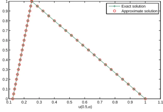
Figure 1: Graph of the VIM approximation error of Numerical illustration for example 5.1.
Example 5.2. Consider the pantograph equation of first order with variable coefficients
{
u′gH(t) =⊖gHu(t)⊖gHe
−t 2 sin(t
2)u(
t
2)⊖gH2e −3t
4 cos(t
2)sin(
t
4)u(
t
4), 0≤t≤1;
u(0;α) = [α+1 −2α+4], for allα∈[0,1]. Note that the exact solution of this problem is
u(t;α) = [α+1 −2α+4]e−tcos(t)
Since u(t)has (ii)-gH-differentiable, the (ii)-gH-differentiable solution is obtained by solving
u′(t;α) =−u(t;α)−e−2tsin(t
2)u(
t
2;α)−2e −3t
4 cos(t
2)sin(
t
4)u(
t
4;α);
u′(t;α) =−u(t;α)−e−2tsin(t
2)u(
t
2;α)−2e −3t
4 cos(t
2)sin(
t
4)u(
t
4;α);
u(0;α) = [α+1 −2α+4]
To solve this equation using the VIM, based on the iteration formula (3.11) we get
un+1(t;α) = un(t;α)−
∫ t
0
e(s−t)[u′(s;α) +u(s;α) +e−2ssin(s
2)u(
s
2;α) +2e −3s
4 cos(s
2)sin(
s
4)u(
s
4;α)
]
ds (5.16)
un+1(t;α) = un(t;α)−
∫ t
0
e(s−t)[u′(s;α) +u(s;α) +e−2ssin(s
2)u(
s
2;α) +2e −3s
4 cos(s
2)sin(
s
4)u(
s
4;α)
]
ds (5.17)
We start with initial approximation u0(t;α) = (α+1)cos(t)and u0(t;α) = (−2α+4)cos(t), the other terms of the sequence un(t;α)are computed easily by substituting this equation into Eqs. (5.16) and (5.17), we have
n=1
u1(t;α) = (α+1)−(α+1)t+ 5
24(α+1)t 3+
...
u1(t;α) = (−2α+4)−(−2α+4)t+ 5
24(−2α+4)t 3+
...
n=2
u2(t;α) = (α+1)−(α+1)t+1
3(α+1)t 3−1
6(α+1)t
4+ 539
15360(α+1)t 5+
...
u2(t;α) = (−2α+4)−(−2α+4)t+1
3(−2α+4)t 3−1
6(−2α+4)t
4+ 539
15360(−2α+4)t 5+
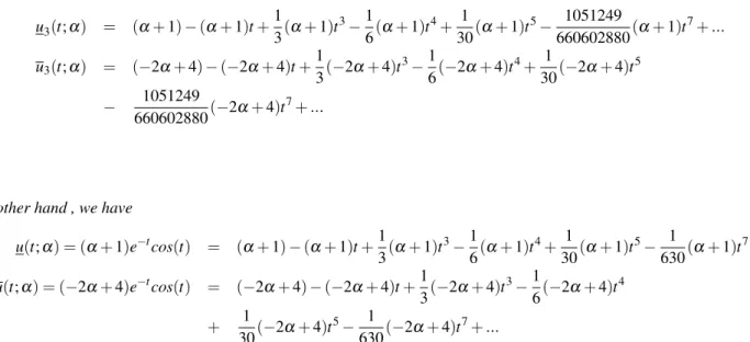
n=3
u3(t;α) = (α+1)−(α+1)t+1
3(α+1)t 3−1
6(α+1)t 4+ 1
30(α+1)t
5− 1051249
660602880(α+1)t 7+...
u3(t;α) = (−2α+4)−(−2α+4)t+1
3(−2α+4)t 3−1
6(−2α+4)t 4+ 1
30(−2α+4)t 5
− 1051249
660602880(−2α+4)t 7+
...
.. .
In the other hand , we have
u(t;α) = (α+1)e−tcos(t) = (α+1)−(α+1)t+1
3(α+1)t 3−1
6(α+1)t 4+ 1
30(α+1)t 5− 1
630(α+1)t 7+...
u(t;α) = (−2α+4)e−tcos(t) = (−2α+4)−(−2α+4)t+1
3(−2α+4)t 3−1
6(−2α+4)t 4 + 1
30(−2α+4)t 5− 1
630(−2α+4)t 7+...
We see that the approximation solutions obtained by VIM have good agreement with exact solution of this problem. In Table 2 the absolute errors of the present method for n=3andα=1
3.
α=1 3
t u3(t,13) u3(t,13)
1 3.70000×10⁻¹³ 6.70000×10⁻¹³ 2 4.88800×10⁻¹¹ 3.94567×10⁻¹⁰ 3 6.50702×10⁻⁹ 2.52618×10⁻⁹ 4 2.50932×10⁻⁸ 5.24619×10⁻⁸
5 6.98447×10⁻⁸ 6.47814×10⁻⁷ 6 1.96801×10⁻⁷ 5.73890×10⁻⁷ 7 2.65590×10⁻⁷ 6.32457×10⁻⁶ 8 4.87889×10⁻⁷ 3.00921×10⁻⁷
0.4 0.6 0.8 1 1.2 1.4 1.6 1.8 2 2.2 2.4 0
0.1 0.2 0.3 0.4 0.5 0.6 0.7 0.8 0.9 1
u(0.5,α)
α
Exact solution Approximate solution
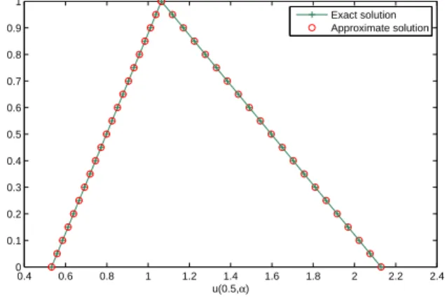
Figure 2: Graph of the VIM approximation error of Numerical illustration for example 5.2
6 Conclusion
In this paper, we proposed the variation iteration method for solve the fuzzy generalized pantograph equation under generalized Hukuhara differentiability concept. First we choose type of differentiability of solution and convert it to a system of differential equations. Then we use VIM and find the approximate solution of this system. This technique produces the terms of a sequence using the iteration of the correction functional which converges to the exact solution rapidly.
References
[1] S. Abbasbandy, T. Allahviranloo, Numerical solutions of fuzzy differential equations by taylor method, Compu-tational Methods in Applied Mathematics, 2 (2002) 113-124.
http://dx.doi.org/10.2478/cmam-2002-0006
[2] S. Abbasbandy, T. Allahviranloo, O. Lopez-Pouso, J. J. Nieto, Numerical methods for fuzzy differential inclu-sions, Computer and Mathematics With Applications, 48 (10-11) (2004) 1633-1641.
http://dx.doi.org/10.1016/j.camwa.2004.03.009
[3] T. Allahviranloo, N. Ahmady, E. Ahmady, Erratum to Numerical solution of fuzzy differential equations by predictor-corrector method, Information Sciences, 178 (2008) 1780-1782.
http://dx.doi.org/10.1016/j.ins.2007.11.009
[4] T. Allahviranloo, N. Ahmady, E. Ahmady, Numerical solution of fuzzy differential equations by predictor-corrector method, Information Sciences, 177 (7) (2007) 1633-1647.
http://dx.doi.org/10.1016/j.ins.2006.09.015
[5] T. Allahviranloo, A. Armand, Z. Gouyandeh, H Ghadiri, Existence and uniqueness of solutions for fuzzy frac-tional Volterra-Fredholm integro-differential equations, Journal of Fuzzy Set Valued Analysis, 2013 (2013) 1-9.
http://dx.doi.org/10.5899/2013/jfsva-00163
[7] T. Allahviranloo, Z. Gouyandeh, A. Armand, Fuzzy fractional differential equations under generalized fuzzy Caputo derivative, Journal of Intelligent and Fuzzy Systems, (In press).
[8] T. Allahviranloo, N. A. Kiani, M. Barkhordari, Toward the existence and uniqueness of solutions of second-order fuzzy differential equations, 179 (8) (2009) 1207-1215.
http://dx.doi.org/10.1016/j.ins.2008.11.004
[9] A. Armand, Z. Gouyandeh, Numerical solution of the system of Volterra integral equations of the first kind, International Journal of Industrial Mathematics, 6 (1) 27-35.
[10] A. Armand, Z. Gouyandeh, Solving two-point fuzzy boundary value problem using variational iteration method, Communications on Advanced Computational Science with Applications, 2013 (2013) 1-10.
http://dx.doi.org/10.5899/2013/cacsa-00006
[11] B. Bede, I. J. Rudas, A. L. Bencsik, First order linear fuzzy differential equations under generalized differentia-bility, Information Sciences, 177 (2007) 1648-1662.
http://dx.doi.org/10.1016/j.ins.2006.08.021
[12] B. Bede, L. Stefanini, Generalized differentiability of fuzzy-valued functions, Fuzzy Sets and Systems, 230 (2013) 119-141.
http://dx.doi.org/10.1016/j.fss.2012.10.003
[13] J. J. Buckley, Simulating Continuous Fuzzy Systems, Springer, (2006).
[14] J. J. Buckley, T. Feuring, Introduction to fuzzy partial differential equations, Fuzzy Sets and Systems, 105 (1999) 241-248.
http://dx.doi.org/10.1016/S0165-0114(98)00323-6
[15] S. L. Chang, L. A. Zadeh, On fuzzy mapping and control, IEEE Transactions on Systems Man Cybernetics, 2 (1972) 330-340.
[16] W. Congxin, S. Shiji, Existence theorem to the Cauchy problem of fuzzy differential equations under compactness-type conditions, Information Sciences, 108 (1998) 123-134.
http://dx.doi.org/10.1016/S0020-0255(97)10064-0
[17] G. A. Derfel, F. Vogl, On the asymptotics of solutions of a class of linear functional-differential equations, European J. Appl. Math, 7 (1996) 511-518.
http://dx.doi.org/10.1017/S0956792500002527
[18] Z. Ding, M. Ma, A. Kandel, Existence of the solutions of fuzzy differential equations with parameters, Informa-tion Sciences, 99 (1997) 205-217.
http://dx.doi.org/10.1016/S0020-0255(96)00279-4
[19] D. Dubois, Towards fuzzy differential calculus: part 3, differentiation, Fuzzy Sets and Systems, 8 (1982) 225-233.
http://dx.doi.org/10.1016/S0165-0114(82)80001-8
[20] A. Feldstein, Y. Liu, On neutral functional-differential equations with variable time delays, Math. Proc. Cam-bridge Philos. Soc, 124 (1998) 371-384.
http://dx.doi.org/10.1017/S0305004198002497
[21] Z. Gouyandeh, A. Armand, Numerical solutions of fuzzy linear system differential equations and application of a Radioactivity decay model, Communications on Advanced Computational Science with Applications, 2013 (2013) 1-11.
[22] J. H. He, Approximate solution of nonlinear differential equations with convolution product non-linearities, Comput. Methods. Appl. Mech. Engrg, 167 (1998) 69-73.
http://dx.doi.org/10.1016/S0045-7825(98)00109-1
[23] J. H. He, Variational iteration method for delay differential equations, Commun. Nonlinear. Sci. Numer. Simul, 2 (1997) 235-236.
http://dx.doi.org/10.1016/S1007-5704(97)90008-3
[24] M. Inokuti, H. Sekine, T. Mura, General use of the Lagrange multiplier in non-linear mathematical physics, in: Variational Methods in the Mechanics of Solids, Pergamon Press, Oxford, (1978) 156-162.
[25] L. J. Jowers, J. J. Buckley, K. D. Reilly, Simulating continuous fuzzy systems, Information Sciences, 177 (2007) 436-448.
http://dx.doi.org/10.1016/j.ins.2006.03.005
[26] O. Kaleva, Fuzzy differential equations, Fuzzy Sets and Systems, 24 (1987) 301-317.
http://dx.doi.org/10.1016/0165-0114(87)90029-7
[27] O. Kaleva, The Cauchy problem for fuzzy differential equations, Fuzzy Sets and Systems, 35 (1990) 389-396.
http://dx.doi.org/10.1016/0165-0114(90)90010-4
[28] N. Mikaeilvand, L. Hossieni, The Taylor Method for Numerical Solution of Fuzzy Generalized Pantograph Equations with Linear Functional Argument, Int. J. Industrial Mathematics, 2 (2) (2010) 115-127.
[29] G. R. Morris, A. Feldstein, E. W. Bowen, The Phragmen-Lindel of principle and a class of functional-differential equations, in Proceedings of NRL-MRC Conference on Ordinary Differential Equations, (1972) 513-540.
[30] J. R. Ockendon, A. B. Tayler, The dynamics of a current collection system for an electric locomotive, Proc. Roy. Soc. London Ser. A, 322 (1971) 447-468.
http://dx.doi.org/10.1098/rspa.1971.0078
[31] S. Seikkala, On the fuzzy initial value problem, Fuzzy Sets and Systems, 24 (1987) 319-330.