Multi-Objective Fuzzy Linear Programming In Agricultural Production Planning

242

_______________________

 H.M.I.U. Herath, Department of Mathemetics, Faculty of Sciene, University of Peradeniya.

 Dr. D.M. Samarathunga, Department of Mathemetics,

Faculty of Sciene, University of Matara.

Multi-Objective Fuzzy Linear Programming In

Agricultural Production Planning

H.M.I.U. Herath, Dr. D.M. Samarathunga

Abstract: Modern agriculture is characterized by a series of conflicting optimization criteria that obstruct the decision-making process in the planning of agricultural production. Such criteria are usually net profit, total cost, total production, etc. At the same time, the decision making process in the agricultural production planning is often conducted with data that accidentally occur in nature or that are fuzzy (not deterministic). Such data are the yields of various crops, the prices of products and raw materials, demand for the product, the available quantities of produc tion factors such as water, labor etc. In this paper, a fuzzy multi-criteria mathematical programming model is presented. This model is applied in a region of 10 districts in Sri Lanka where paddy is cultivated under irrigated and rain fed water in the two main seasons called ―Yala‖ and ―Maha‖ and the optimal production plan is achieved. This study was undertaken to find out the optimal allocation of land for paddy to get a better yield while satisfying the two conflicting objectives; profit maximizing and cost minimizing subjected to the utilizing of water constraint and the demand constraint. O nly the availability of land constraint is considered as a crisp in nature while objectives and other constraints are treated as fuzzy. It is observed that the MOFLP is an effective method to handle more than a single objective occurs in an uncertain, vague environment.

Index Terms: Multi-objective fuzzy linear programming, membership function, tolerance variables.

————————————————————

1 INTRODUCTION

THE first and most significant motivation towards the mathematical formalization of fuzziness was initiated by Lofti A. Zadeh in 1960’s. Zadeh has made novel contribution with his papers for the development, propagation and application of fuzzy logic to the real world problems. Fuzzy set theory provides a strict mathematical framework in which vague concepts can be precisely studied. Its further development is in progress, with numerous attempts being made to explore the ability of fuzzy set theory to become a useful tool for mathematical analysis of real world problems. Recent applications to various scientific fields such as precision machinery, artificial intelligence, image processing, decision theory, military science, medical science, sociology, economics, psychology, biology, management science, and Expert Systems, Control Theory, Mathematics and Statistics have demonstrated that fuzzy set theory may not be a theory in search of applications, but indeed a useful tool for the expressions of professional judgments. Bellman and Zadeh [2] (1970) have focused on the concept of decision making in a fuzzy environment. They considered the classical model of a decision and suggested a model for decision making under uncertainty in which the objective function as well as the constraint(s) are fuzzy. They made the argument saying that the fuzzy objective function is characterized by its membership function, and so are the constraints. The first formulation of Fuzzy Linear Programming is proposed by Zimmermann in 1976 [3], [4.] Thereafter, many authors considered various types of the fuzzy linear programming problems and proposed several approaches for solving these problems. Zimmermann introduced fuzzy linear programming as conventional LP. He considered LP problems with a fuzzy goal and fuzzy constraints and used linear membership functions and the min operator as an aggregator for these functions. In many real

world problems determining "optimal" solutions cannot be done by using a single criterion or a single objective function. This area, multi-criteria decision making, has led to numerous evaluation schemes and to the formulation of vector-maximum problems in mathematical programming. The Multi-Objective Decision Making (MODM) problem is often called the "vector maximum" problem, and was first mentioned by Kuhn and Tucker (1951). In this paper MODM is studied in the area of Agricultural Production Planning(APP). They deal with cost and profit while utilizing the resources in order to satisfy the demand. When solving APP problems it is often assumed that the input data are deterministic/crisp. But in practice, they are usually imprecise or rather fuzzy. The difficulty of fitting accurate parameters is due to obtaining them through approximation or human observations. Therefore finding an optimal solution under this assumption may not be practical. A small violation in constraints and conditions may lead to a more efficient solution. The concept of fuzzy is adopted in such situations. Fuzzy APP allows the vagueness that exists in the determining forecasted demand and the parameters associated with cost of production, available resources such as water, labor and machinery. Fuzzy set theory increases the model realism and enhances the implementation of APP models in industry. The usefulness of fuzzy set theory also extends to multiple objective APP models where additional imprecision due to conflicting goals may enter into the problem.

2.0

METHODOLOGY

2.1

Multi-Objective optimization problem

In most of the decision making problems in real world the decision maker has to often optimize more than one conflicting objectives subject to some constraints.

In general,

   

 





 

 

0

1 ...,

, 2 , 1 0

..., , , ₂ 1



 

x

q i

x g

to subject

x Z x Z x Z Maximize

i

p

Where,x



x₁,x₂,...,x_n



n andZ_i

 

x, j1,2,...,pare

243

model of a multi objective optimization problem withp number of objectives to be maximized subject to qnumber of constraints. In real world problems most of the times there can be objectives to be maximized as well as to be minimized.

2.2

Fuzzy approach

Fuzzy logic (FL) is a mathematical technique for dealing with imprecise data and problems that have many solutions rather than one. Fuzzy logic enables approximate human reasoning capabilities to be applied to knowledge-based systems and provides a mathematical strength to capture the uncertainties associated with human cognitive processes, such as thinking and reasoning.

2.3

Fuzzy set theory

It was specifically designed to represent uncertainty and vagueness mathematically and to provide formalized tools for dealing with the imprecision intrinsic to many problems. Informally, a set is known as fuzzy if the existence or the belongingness of an element to the set is not certain. A formal definition is given as follows:

Definition 1

Let X be a nonempty set. A fuzzy set A in Xis characterized by its membership function _A

 

x :X[0,1]and

 

x A

 is interpreted as the degree of membership of element

xin fuzzy set A for eachxX. _{Then a fuzzy set} A in X is a set of ordered pairs: A





x,A

 

x



:xX



The range of the membership function is [0,1] and the value zero is used to represent complete non-membership, the value one is used to represent complete membership, and values in between are used to represent intermediate degrees of membership.

2.4

Types of membership functions

The selection of a suitable membership function for a fuzzy set is one of the most important activities in fuzzy logic. It is the responsibility of the user to select a function that is a best representation for the fuzzy concept to be modeled. The most commonly used membership functions are the following (Dubois and Prade, 1980; Zimmermann, 1996):

 linear membership function  triangular membership function  trapezoid membership function  sigmoid membership function  ∏-type membership function  Gaussian membership function

The monotonically increasing linear membership function (figure 1) is given by

Fig 1

The monotonically decreasing linear membership function (figure 2) is given by

The triangular membership function (figure 3) is given by

 

  

   

 

   



  







   

 

  

 





x x x

x x

x

x

if if if if

0 0

Fig 3

The trapezoid membership function (figure 4) is given by

 

   

    

 

   



 

  







   

 

 

  

 





x x x

x x x

x

x

if 0

if if 1

if if 0

Fig 4

2.6

Fuzzy linear Programming

In Bellman and Zadeh’s approach of fuzzy LP the goals and the constraints are represented by fuzzy sets and then aggregate them in order to derive a maximizing decision. In contrast to classical Linear Programming, Fuzzy Linear Programming is not uniquely defined in which many variations are acceptable. Consider the following classical LP model

Z

 

x C x

T  max

s.t. ₍₂₎ AxT b

x0

Where, C,xn,bm and Amn. Now make the Assumptions that,

 All coefficients of A,b and C are real (crisp) numbers and  is meant in a crisp sense.

 Any violation of any single constraint renders the solution infeasible.

 All constraints are of equal importance (weights).

In fact, these are rather unrealistic assumptions which are partly relaxed in fuzzy LP space. Now, if LP decision has to be made in a fuzzy environment the decision maker might rather want to reach some aspiration levels instead of maximizing the objective function. These aspiration levels

 

     

   







   



 



x x x

x x

if 0

if if 1

Fig 2

 

     

   

 



    

 



x x x

x

x

if 0

244

may not be even defined crisply and the constraints may also be vague and  sign might not be meant in the strictly mathematical sense but small violations are acceptable. Also, the coefficients of the vectors b or Cor matrix A itself can contain a fuzzy characters because they are fuzzy in nature. Moreover, the constraints might be of different importance or possible violations of different constraint may be acceptable in different degrees.

7.0

Multi-objective Fuzzy Linear Programming

The problem of finding an optimal solution in a fuzzy environment becomes more complicated if several objective functions exist. This leads to the area of multi-criteria fuzzy programming analysis. This area has grown very much since the 1970s. Many approaches have been suggested to solve problems with several objective functions. In all these approaches, objective functions were considered to be real valued and the actions as crisply defined. In general, a multi objective optimization problem with k objectives to be maximized and m objectives to be minimized subject top constraints with ndecision variables is as follows:

 

 

. . min max t s x Z x Z m m k k (3)

�_�(�)≤ �_� i1,2,...,p x0

Where,x



x1,x2,...,xn



n,Zk

 

x and Zm

 

x are objective

functions. If all the objective functions and constraints of above model are fuzzy then its fuzzy model of can be rewritten as:

�_� � �_�0 �_� � �_�0

s.t. ₍₄₎

�_� � �_� i1,2,...,p x0

Where, 0 k

Z and 0 m

Z are the aspiration levels of the goals. Then the fuzzy set decision D is then defined as,

 

 

 

 

_

 

 x x x

x

i m

k Z g

Z i m k

D   

 min , ,

, ,

(5)

Where,

 

x

k Z

 and

 

x

m Z

 are the membership functions of

the objectives and

 

x

i g

 is the membership function of the constraints. Then the optimal decision is the solution which can maximize the minimum attainable aspiration levels. Therefore the optimal solution is given by,

 

 

 



x x x



D

 

x

x g Z Z i m k

x 0 , ,  k  m  i 0 max , , min max 

  (6)

By applying a suitable membership function the optimal solution can be obtained. In this paper linear membership function is adopted. So the model can be modified as follows: Let t_k,t_m,t_i for i1,2,...,p be the subjectively chosen constants of admissible violation of the objective function and constraints respectively. Then the membership function for the objective is given by

 

 

 





_{ }

 

                k k k k k k k k k k k k k Z t Z x Z if Z x Z t Z if t t Z x Z Z x Z if x k 0 0 0 0 0 0 1

 (7)

 

 





 

_{ }

 

                m m m m m m m m m m m m m Z t Z x Z if t Z x Z Z if t x Z t Z Z x Z if x m 0 0 0 0 0 0 1  (8)

The membership function for theithconstraint is given by

 

 





 

_{ }

 

               i i i i i i i i i i i i i g t b x g if t b x g b if t x g t b b x g if x i 0 1

 (9)

Introducingas  _

 

x

 

x

 

x _

i m

k Z g

Z i m k   

 min , ,

,

, then the crisp

equivalent of the MOFLP model is:

 

 

 

0 ..., , 2 , 1 . . max 0 0            x p i t b t x g t Z t x Z t Z t x Z t s i i i i m m m m k k k k for     (10)

If the solution of (10) is the vector

 

*,x* thenx* is considered as the best compromise solution and * is interpreted as the degree of reality (or achievability of x*).

2.8

Degree of satisfaction (λ)

, represented in the above model (10) is known as the degree of satisfaction or degree of achievability of x*. It is the minimum attainable level in the fuzzy system. The upper and the lower bounds of  reflect two extreme scenarios in the system. The upper bound 1indicates that all the goals have been completely satisfied and therefore represents a no confliction occurs among them. The lower bound 0 indicates that at least one goal has a zero satisfaction level and therefore represents a conflict scenario. Any intermediate value between 0 and 1 represents the level of satisfaction in the system. The multi objective fuzzy linear programming aims at achieving a fair compromise solution by increasing the degree of satisfaction λ in the system.

2.9

Computational algorithm

The solution procedure of Multi-Objective Fuzzy Linear Programming can be briefly stated as follows:

1) Solve the very first LPP using linear programming techniques taking one objective function with constraints at a time while ignoring the other probabilistic cases.

245

3) From step 2, obtain the lower and upper bounds and for each objective functions and construct a table of positive ideal solutions

4) Formulate the linear membership functions for each fuzzy goal.

5) Formulate the crisp equivalent of the fuzzy Linear Programming model.

6) Obtain the compromise solution with highest degree of satisfaction.

3.0

AGRICULTURAL PRODUCTION PLANNING

3.1

General model formulation

The decision variables are defined as followsx_ijkl  The area of land cultivated extent in district iin season junder water regimekof variety of paddy l



i Index for the district i



1,2,...,I





j Index for the season j



1,2,...,J





k Index for the water regime k



1,2,...,K





l Index for the variety of paddy l



1,2,...,R



3 conflicting objective functions and the constraints are expressed as follows:

Objectives / Goals

1) Minimize the cost of production i) Labor

ii) Material – seeds, fertilizer iii) Power - machinery 2) Maximize the yield 3) Maximize the profit

Constraints

1) Land 2) Water 3) Labor 4) Machine

5) Demand

Let the parameters be defined as follows: 

ijkl

C Cost of production (labor, material, power) per unit area in district i in season j under water regime k of variety of paddyl.

 ijkl

Y Amount of average yield produced per unit area in district i in season j under water regime k of variety of paddyl.

 ijkl

P Profit gained per unit area in district i in season j

under water regime k of variety of paddyl.

 ijkl

a Lower bound for the decision variable. 

ijkl

b Total cultivable land in district i in season j under water regime k of variety of paddyl.

 ijkl

w Water requirement per unit area in district i in season

j _{under water regime k of variety of paddyl.}

 ijk

W Amount of water available for agriculture purpose in district i in season j under water regime k of variety of paddyl.

 ijkl

L Labor hours required per unit area in district i in season j under water regime k of variety of paddyl.

 i

TL Total labor hours available in districti. 

ijk

m Machine hours required per unit area in district i in season j under water regime k of variety of paddyl.

 i

M Total machine hours available in districti.



TP Total production target.

 l

d Demand for each variety.

3 conflicting objective functions and the constraints are expressed as follows:

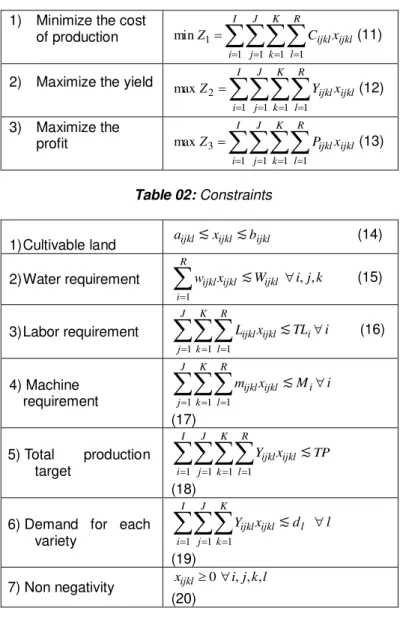
Table 01: Objective functions

1) Minimize the cost

of production



   

 I i

J

j K

k R

l

ijkl ijklx

C Z

1 1 1 1 1

min (11)

2) Maximize the yield



   

 I

i J

j K

k R

l

ijkl ijklx

Y Z

1 1 1 1 2

max (12)

3) Maximize the

profit



   

 I

i J

j K

k R

l

ijkl ijklx

P Z

1 1 1 1 3

max (13)

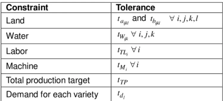
Table 02: Constraints

1)Cultivable land aijkl xijkl bijkl (14) 2)Water requirement





R

i

ijkl ijklx

w

1

k j i

W_ijkl , , (15)

3)Labor requirement



  

J

j K

k R

l

ijkl ijklx

L

1 1 1

i

TL_i (16)

4)Machine

requirement



  

J

j K

k R

l

ijkl ijklx

m

1 1 1

i M_i (17)

5)Total production

target



   

I

i J

j K

k R

l

ijkl ijklx

Y

1 1 1 1

TP

(18)

6)Demand for each

variety



  

I

i J

j K

k

ijkl ijklx

Y

1 1 1

l dl 

(19)

246

Fig 8 – Location map of districts under study

3.2

Method of solving

Using the procedure mentioned previously by solving the MOLPP taking one objective at a time upper and lower bounds for each objective can be found. Now let the aspiration levels of the goals cost, production, and profit obtained from the above method, beZC,ZYand ZP

respectively. Further the tolerance levels of these objectives can also be found as tC,tY and tP. Also assign the tolerance

levels for other constraints as follows:

Table 03: Tolerance levels assigned for the constraints

Constraint Tolerance

Land taijkl and tbijkl i,j,k,l

Water t i jk

ijk W  , ,

Labor t i

i TL 

Machine t i

i M 

Total production target tTP

Demand for each variety tdl

Then the crisp equivalent of the fuzzy LP is given by,

1 0 , , , 0 , , , , . . max

1 1 1 1 1 1 1 1 1 1 1 1 1 1 1

1 1 1 1 1 1 1 1 1 1 1 1

                                   



















                                      l k j i x l t d t x Y t TP t x Y i t M t x m i t TL t x L k j i t W t x k j i t a t x t Z t x P t Z t x Y t Z t x C t s ijkl I i K k d l R l d ijkl ijkl I i J j K k R l TP TP ijkl ijkl I i K k M i R l M ijkl ijkl I i K k TL i R l L ijkl ijkl W ijk R l W ijkl R l a ijk a ijkl I i J j K k R l P P P ijkl ijkl I i J j K k R l Y Y Y ijkl ijkl I i J j K k R l C C C ijkl ijkl l l i i i i ijk ijk ijk ijk (21)

This can be easily solved using linear programming techniques.

3.3

Case study

Paddy cultivation in Sri Lanka

Rice is the staple food for more than half of the human population, and in Asia alone more than 2 billion people depend on rice and its products for their food intake. Rice is the single most important crop occupying 34 percent (0.77 million ha) of the total cultivated area in Sri Lanka. On average 560,000 ha are cultivated during Maha and 310,000 ha during Yala making the average annual extent sown with rice to about 870,000 ha. About 1.8 million farm families are engaged in paddy cultivation island-wide. It has become deeply embedded in the cultural heritage of Sri Lankan society. In Sri Lanka paddy is cultivated under 2 seasons namely Yala and Maha. Maha season falls from October to March while Yala season falls from April to September. In each season paddy cultivation is done under 2 water regimes called irrigation and rain fed. As a result of population growth there is a need of more production to satisfy the ever increasing demand. To feed these more consumers production of paddy must be increased. This effort must be carried out against a backdrop of decreasing available arable land, increasing competition for water, labor hours, machine hours and a growing concern for environmental protection and conservation. In the present study optimal land allocation for paddy is described. A general model is presented for the production of paddy and method of solving is explained through multi-objective fuzzy linear programming. To solve the MOFLPP linear membership function is considered. Here, all the objective functions and constraints are treated as fuzzy except for the land constraint. For the case study paddy cultivation in 10 districts (Ampara,

Anuradhapura, Hambanthota, Kurunegala, Mannar,

Polonnaruwa, Trincomalee, Gampaha, Kalutara, Kandy) is considered under some assumptions. The case study is presented by the data obtained from the Department of Agriculture (Cost of cultivation 2012 Yala and Maha)

According to the data obtained from the Department of agriculture following model can be formulated.

Decision variable

 ijk

x The area of land cultivated extent in district iin season junder water regimek.

247

1) Minimize the cost of production i) Labor

ii) Material- seeds, fertilizer iii) Power- machinery 2) Maximize the profit

Constraints

1) Land 2) Water

3) Demand

Table 04: Information about decision variables in the case study

Table 05: Data per hectare

Table 06: Data per hectare

Table 07: Data of available resources

Table 08: Data of available resources

Total demand for paddy in these 10 districts is 1099244768kg. Using this information mathematical model can be formed.

4.0

R

ESULTS AND DISCUSSION

Using the procedure mentioned in the algorithm following solutions can be obtained by solving the LP by taking one objective at a time.

Table 09: Solution obtained by individual optimization

i District j Season k Water regime

1 Ampara 1 Yala 1 Irrigation

2 Anuradhapura 2 Maha 2 Rain fed

3 Hambanthota

4 Kurunegala

5 Mannar

6 Polonnaruwa

7 Trincomalee

8 Gampaha

9 Kalutara

10 Kandy

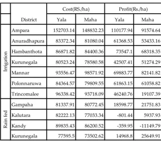
Yala Maha Yala Maha

Ampara 152703.14 148832.23 110177.94 91574.64

Anuradhapura 83372.34 81080.04 61368.53 53433.16

Hambanthota 86871.82 84400.36 73547.1 68318.35

Kurunegala 80523.24 78580.58 42507.41 51274.29

Mannar 93556.47 98571.92 69883.77 82141.82

Polonnaruwa 84364.57 79809.55 61863.15 61058.82

Trincomalee 96338.42 93718.09 46240.76 19107.39

Gampaha 81337.91 80772.45 18598.77 21751.83

Kalutara 82222.13 77033.34 -801.44 5937.93

Kandy 89835.43 86200.52 -359.95 -11149.79

Kurunegala 77595.5 73502.62 14968.8 25649.91 District

Cost(RS./ha) Profit(Rs./ha)

Ir

ri

g

a

ti

o

n

R

a

in

f

ed

Yala Maha Yala Maha

Ampara 10041 9703 5952 5952

Anuradhapura 5682 5761 5952 5952

Hambanthota 6692 6815 5952 5952

Kurunegala 5153 5369 5548 5252

Mannar 6913 7028 5952 5252

Polonnaruwa 5678 6175 5952 5252

Trincomalee 7064 6395 5952 5548

Gampaha 3349 3341 5952 5252

Kalutara 2762 2860 5952 5252

Kandy 3077 2783 5952 5252

Kurunegala 3494 3470 5548 5548 Yield(kg/ha) Water(m^3/ha)

Ir

ri

ga

tio

n

R

ai

n

fe

d

District

District Yala Maha

Ampara 1317095871 1317095871

Anuradhapura 550321623 550321623

Hambanthota 136829849 156829849 Kurunegala 158586944 218586944

Mannar 15003002 16003002

Polonnaruwa 434822084 434822084 Trincomalee 96421506 136421506

Gampaha 183940370 183940370

Kalutara 372355099 372355099

Kandy 96605786 96605786 Kurunegala 621948083 621948083

Available water(m^3)

Irri

g

a

ti

on

Ra

in

fe

d

District Yala Maha Yala Maha Ampara 4100 4300 48202 48202 Anuradhapura 5500 5500 77996 77996 Hambanthota 3750 3575 19087 19087 Kurunegala 10000 10000 35789 35789

Mannar 750 750 11162 11162

Polonnaruwa 2500 3000 60887 60887 Trincomalee 2500 2500 22901 22901

Gampaha 1331 6290 9179 9179

Kalutara 6107 11942 13795 13795

Kandy 497 3619 6991 6991

Kurunegala 5000 5000 23897 23897 Lower bound for

cultivable land (ha)

Total cultivable land (ha)

Irri

g

a

ti

on

Ra

in

fe

248

Now identify the upper and lower bounds for each of the objectives from the solutions obtained when solving the LP by taking one objective at a time. From these bounds tolerance values of the cost objective and profit objective can be found.

Tolerance for cost objective 56,968,716,134.03- 16,321,893,649.01  40,646,822,485.01

Tolerance for profit objective 34,882,583,647.94-9,923,240,370.41  24,959,343,277.53

Also, following values are assigned for the tolerance of other fuzzy constraints. Here the land constraint is considered as a crisp one.

Table 11: Tolerance values for water constraints

Table 12: Tolerance value for demand constraint

Using these values crisp equivalent of the fuzzy LP can be formulated and then solved using any method used to solve LP models. Now by using the method of Fuzzy multi-objective linear programming a compromise solution is obtained as follows.

Table 13: Compromise solution for the fuzzy LP

Final answer for cost, profit objectives and demand constraint can be stated as follows:

Cost objective = Rs. 22,023,946,784.83 Profit objective = Rs. 9,923,240,370.41 Demand constraint = 1249143590 kg

The overallvalue is zero as some of the membership function values are zero. In the compromise solution it can be seen that in some of the districts almost all the available land is cultivated while in some of them the answer is just the lower bound. By computing the value of the membership function for each fuzzy objectives and constraints a clear idea can be obtained about how much they are satisfied.

Table 14: Membership values for the objectives and constraints

Table 15: Membership values for the water constraints

Membership value for cost objective is 0.86. That means the objective is satisfied 86%. As in the problem the government would like to spend Rs.16,321,893,649.01 for paddy production in a year. But the answer shows that the total production cost is Rs.22,023,946,784.83. that is the

Total c ost(Rs) Total profit(Rs) Demand(kg)

Yala (ha) Maha (ha) Yala (ha) Maha (ha)

Ampara 4100 4300 48202 48202

Anuradhapura 5500 5500 77996 77996

Hambanthota 19087 19087 19087 19087

Kurunegala 10000 10000 28587 35789

Mannar 2521 750 2521 2689

Polonnaruwa 2500 60887 60887 60887

Trinc omalee 5464 2500 16199 22901

Gampaha 1331 6290 9179 9179

Kalutara 6107 11942 6107 13795

Kandy 497 3619 497 3619

Kurunegala 5000 5000 23897 23897

1099244768 3756222195

Distric ts

Cultivated extent

Ir

ri

g

a

ti

on

R

a

in

f

ed

Minimize cost Maximize profit 16,321,893,649.01 56,968,716,134.03

9,923,240,370.41 34,882,583,647.94

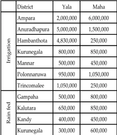
District Yala Maha

Ampara 2,000,000 6,000,000

Anuradhapura 5,000,000 1,500,000

Hambanthota 4,830,000 250,000

Kurunegala 800,000 850,000

Mannar 500,000 450,000

Polonnaruwa 950,000 1,050,000

Trincomalee 1,050,000 250,000

Gampaha 500,000 800,000

Kalutara 650,000 850,000

Kandy 400,000 450,000

Kurunegala 300,000 600,000

Irri

g

a

ti

on

Ra

in

fe

d

Target Tolerance

Demand(kg) 1099244768 56857488

Yala Maha

Ampara 48202 27511

Anuradhapura 5500 5500

Hambanthota 3750 3575

Kurunegala 10000 10000

Mannar 750 2764

Polonnaruwa 2500 3000

Trincomalee 2500 2500

Gampaha 1331 6290

Kalutara 6107 11942

Kandy 497 3619

Kurunegala 5000 5000 District

Cultivated extent(ha)

Ir

ri

g

a

ti

o

n

R

a

in

f

ed

Objective/Constraint Membership value

Cost objective 0.86

Profit objective 0

Demand constraint 1

District Yala Maha Ampara 1 1 Anuradhapura 1 1 Hambanthota 1 1 Kurunegala 1 1 Mannar 1 0 Polonnaruwa 1 1 Trincomalee 1 1 Gampaha 1 1 Kalutara 1 1 Kandy 1 1 Kurunegala 1 1

Ir

ri

g

a

ti

o

n

R

a

in

f

249

government has to pay an additional cost of Rs.5,702,053,135. The membership value for the demand constraint is 1. That means these districts will produce paddy to meet the country’s demand and according to the solution, there is even an excess of production. Table no 14 and 15 give the values for the membership function of each fuzzy constraint and objective. In all the districts for both seasons (accept Mannar in Maha season) the membership function value of water constraint is 1, which means that the available water has been sufficient for the cultivation. That is, no more additional water is expected in these districts. But in Mannar Maha season the constraint take the value of its upper bound in the compromise solution and therefore results with zero membership value. In other words all the available water and the additional water (tolerance level) is also used to produce enough yield in order to meet the country’s demand for rice.

5.0

CONCLUSION

Here, the tolerance values assigned for the fuzzy constraints can be modified according to the decision maker’s preference. That can be done by paying attention on the membership values of the fuzzy constraints/objectives in order to obtain an improved satisfactory solution. In this particular case study, it is important to consider the production cost and the availability of water for agricultural purposes in Mannar district in Maha season as the solution result zero value for the membership functions. So Multi Objective Fuzzy Linear Programming is a more suitable approach to tackle vagueness in planning multiple objectives. It offers a powerful means of handling optimization problems with fuzzy parameters. Since the agricultural problems always come with fuzzy environment MOFLP is a better technique to get a more effective solution. Also it can be noted that by changing the type of the membership function more effective solution can be obtained.

6.0

A

CKNOWLEDGMENT

The author wish to thank Dr. D. M. Samarathunga for his supervision and guidance and members of Census and Statistics section, Department of Agriculture, Sri Lanka.

7.0

REFERENCES

[1] Department of Agriculture- Cost of cultivation of agricultural crops 2012 Yala and 2011/12 Maha.

[2] R.E. Bellman, L. A. Zadeh, Decision making in a fuzzy environment, Management Science 17(1970), B141-164.

[3] H.-J. Zimmermann Fuzzy Set Theory and Its Applications Fourth Edition Springer Science + Business Media, LLC

[4] H.-J. ZIMMERMANN INFORMATION SCIENCES

36,29-58 (1985) 29 Applications of Fuzzy Set theory to Mathematical Programming

[5] Dinesh K. SHARMA, R. K. JANA and Avinash GAUR Yugoslav Journal of Operations Research 17 (2007), Number 1, 31-42

[6] Mostafa Mardani, Alireza Keikha International Journal of Agronomy and Plant Production. Vol., 4 (12), 3419-3424, 2013.

[7] S. K. Bharati, S. R. Singh International Journal of Computer Applications (0975 – 8887) Volume 89– No.6, March 2014

[8] Mohammed. Mekidiche, Mostefa Belmokaddem and Zakaria Djemmaa I.J. Intelligent Systems and Applications, 2013, 04, 20-29

[9] I. Elamvazuthi , T. Ganesan, P. Vasant and J. F. Webb (IJCSIS) International Journal of Computer Science and Information Security, Vol. 6, No. 3, 2009

[10] Anjeli Garg , Shiva Raj Singh Department of Mathematics, Banaras Hindu University, VARANASI- 221005, INDIA

[11] S.A. Mohaddes and Mohd. Ghazali Mohayidin Agricultural American-Eurasian J. Agric. & Environ. Sci., 3 (4): 636-648, 2008 ISSN 1818-6769

[12] Thomas BOURNARIS, Jason PAPATHANASIOU,

Christina MOULOGIANNI , Basil MANOS NEW MEDIT N. 4/2009

[13] A B Mirajkar and P L Patel Proceedings of the 10th Intl. Conf.on Hydro science & Engineering, Nov. 4-7, 2012, Orlando, Florida, U.S.A.

[14] Ritika Chopra1, Ratnesh R. Saxena American Journal of Operations Research, 2013, 3, 65-69

[15] Amit Kumar, Jagdeep Kaur and Pushpinder Singh International Journal of Applied Mathematics and Computer Sciences 6:1 2010

[16] C. Stanciulescu , Ph. Fortemps , M. Install_e , V. Wertz European Journal of Operational Research 149 (2003) 654–675

[17] Salah R. Agha. Latifa G. Nofal, Hana A. Nassar, Rania Y. Shehada Management 2012, 2(4): 96-105 DOI: 10.5923/j.mm.20120204.03

[18] M. R. SAFI, H. R. MALEKI AND E. ZAEIMAZAD Iranian Journal of Fuzzy Systems Vol. 4, No. 2, (2007) pp. 31-45

[19] Sreekumar and S. S. Mahapatra African Journal of Business Management Vol.3 (4), pp. 168-177, April, 2009

[20] S. K. Bharatiand and S. R. Singh International Journal of Modeling and Optimization, Vol. 4, No. 1, February 2014

[21] Waiel F. Abd El-Wahed, Sang M. Lee Omega 34 (2006) 158 – 166

250