EUROPEAN INFLATION-LINKED BONDS: AN HISTORICAL
OVERVIEW AND THE BENEFITS AMID PORTFOLIO
MANAGEMENT
João Pedro Robalo Martins
Project submitted as partial requirement for the conferral of
Master in Finance
Supervisor:
Prof. Doutor José Carlos Dias, ISCTE Business School, Department of Finance
I
RESUMO
A presente dissertação propõe-se a introduzir de um ponto de vista geral a historia das Inflation-Linked Bonds (ILBs), coloquialmente conhecidas como linkers, dos países Europeus desenvolvidos e com especial enfoque em Franca, Alemanha e Italia sendo que estes são os principais emitentes de linkers excluindo o Reino Unido. Para alem da historia, a mecânica destes instrumentos assim como alguns dos conceitos base relacionados, tal como breakeven inflation rates, serão apresentados de forma a explicar como funcionam as ILBs e providenciam proteção contra a inflação. Adicionalmente, aponta para o estudo de alguns indicadores que ajudem, da perspetiva de um investidor, a concluir sobre os benefícios da inclusão de ILBs num portfolio. As principais conclusões a obter são esperadas estar relacionadas com diversificação e alocação de ativos num portfolio através da analise de correlações com ações e obrigações nominais assim como através de uma abordagem a partir do conceito da fronteira eficiente.
Palavras-Chave: inflation-linked bonds; European and developed markets; correlations and portfolio diversification; asset allocation
II
ABSTRACT
This dissertation proposes to introduce an historical overview on European developed countries’ inflation-linked bonds (ILBs), colloquially known as linkers, with a special focus on France, German and Italian, since these countries are the main issuers of ILBs in the Europe excluding the United Kingdom. Besides from the history, the mechanics of these instruments as well as some key concepts as breakeven inflation rates will be presented showing how do ILBs work and provide inflation risk hedging. Further, this thesis aims to study some indicators that will help to conclude on the benefits of the inclusion of ILBs in a portfolio from the investor’s perspective. The main conclusions are expected to be related with diversification and portfolio asset allocation through the analysis of correlations with equities and nominal bonds as well as through an approach using the mean-variance efficient frontier framework.
Keywords: inflation-linked bonds; European and developed markets; correlations and portfolio diversification; asset allocation
III
ACKNOWLEDGEMENTS
The present study is the result of my MSc. in Finance dissertation at ISCTE Business School. It was carried out during the year of 2014 and 2015, mainly during the summer of 2015. The main focus is on introducing European inflation-linked bonds, a relatively recent brand of securities issued by governments, which belong to the fixed income asset class.
Firstly I would like to thank my supervisor Prof. José Carlos Dias for all the guidance, advices and recommendations throughout all the process, always available and constantly incentivizing excellency in my study.
This thesis is a product of my passion towards the fixed income markets and belongs as much to me as to all my friends and family who always kept me pushing forward. I would like to express a special appreciation to my father, mother and brother, for the constant support in all possible ways as well as my Master’s colleagues João Mendes and Miguel Ucha to who I frequently refer as my Brothers in Arms within finance.
Additionally I would like to thank all the team from the financial department of Caixa Central de Crédito Agrícola Mútuo where I had my first professional experience, especially to Martinho Magalhães for all the knowledge and insights I got from him on the fixed income markets.
Finally, I must thank and refer a very special and dear person to me; Claudia Hernandez Cortes. She was the person that encouraged and supported me the most during the past 3 years of my life, having a constant and sincere preoccupation not only with the present dissertation but also with all aspects of my life. Without her by my side, I am sure this would not have been possible.
IV INDEX RESUMO ... I ABSTRACT ... II ACKNOWLEDGEMENTS ... III INDEX OF TABLES ... V INDEX OF FIGURES ... VI INDEX OF EQUATIONS ... VII GLOSSARY... VIII
1. INTRODUCTION ... 1
2. LITERATURE REVIEW ... 4
2.1. Correlations and volatility ... 4
2.2. Portfolio allocation ... 6
3. HISTORICAL OVERVIEW ... 9
3.1. The Origin of Linkers ... 9
3.2. European Inflation-Linked Bonds ... 11
3.3. How do Linkers work? ... 20
4. DATA ... 25
5. DESCRIPTIVE STATISTICS ... 30
6. METHODOLOGY ... 33
6.1. Fisher Equation ... 33
6.2. Breakeven Inflation Rate ... 34
6.3. Inflation-Linked Bonds Duration ... 35
6.4. Efficient Frontier ... 36
7. ANALYZING ILBS CORRELATIONS AND DIVERSIFICATION POWER ... 38
7.1. Inflation Correlations ... 38
7.2. Asset Classes Correlations ... 40
IV
8. ASSET ALLOCATION ... 46
8.1. Efficient Frontier ... 46
8.2 Nominal vs Inflation-Linked Bonds ... 49
9. CONCLUSIONS ... 53 REFERENCES ... 56 Appendix I ... 58 Appendix II ... 61 Appendix III ... 62 Appendix IV ... 64 Appendix V ... 65
V
INDEX OF TABLES
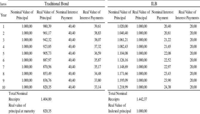
Table 1: Comparing Cash Flows between Traditional and Inflation-Linked Bonds……...…23 Table 2: Key features and Inflation Indices of Major ILBs in Global Markets………...…....29 Table 3: Descriptive Statistics………...………...…30 Table 4: Inflation Correlations by Country and Asset Class………..…..…38 Table 5: Monthly Returns Correlations between the Different Asset Classes………..…..….41 Table 6: ILBs Cross-Country Correlations………..43 Table 7: Nominal Bonds Cross-Country Correlations………...…….….43 Table 8: Equities Cross-Country Correlations………...…….….44 Table 9: Nominal vs Inflation-Linked Bonds in an Equity Portfolio, France…………..…...50 Table 10: Nominal vs Inflation-Linked Bonds in an Equity Portfolio, Germany……..….…51 Table 11: Nominal vs Inflation-Linked Bonds in an Equity Portfolio, Italy…………...52
VI
INDEX OF FIGURES
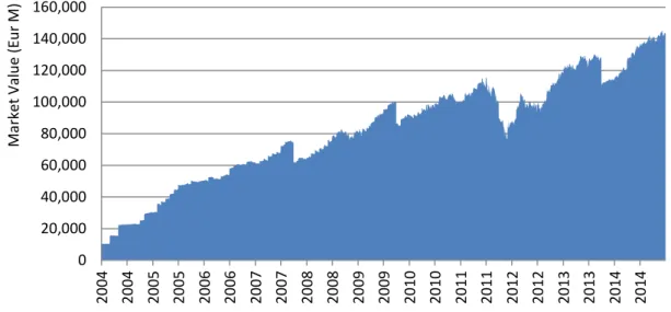
Figure 1: ILBs Indices Evolution by Market Value in Euros………...11
Figure 2: Evolution of the French ILB Market by Market Value……….…………...13
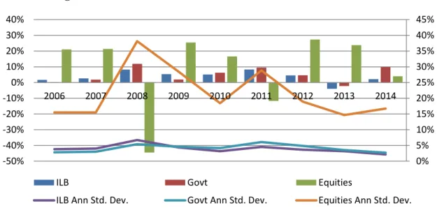
Figure 3: French Market – Historical Performance and Risk………..……14
Figure 4: Evolution of the German ILB Market by Market Value……….………….15
Figure 5: German Market – Historical Performance and Risk………....16
Figure 6: Evolution of the Italian ILB Market by Market Value……….……18
Figure 7: Italian Market – Historical Performance and Risk……….….….19
Figure 8: Comparison between Nominal and Inflation-Linked Bonds’ Structure………..….21
Figure 9: Illustration of ILBs’ Principal and Coupon Mechanics………..……..22
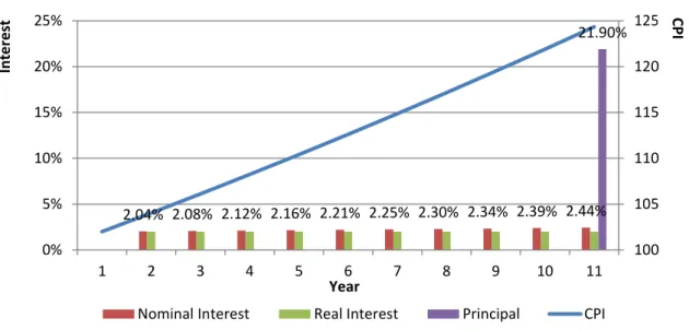
Figure 10: Cash Flow Structure of an ILB………..…….23
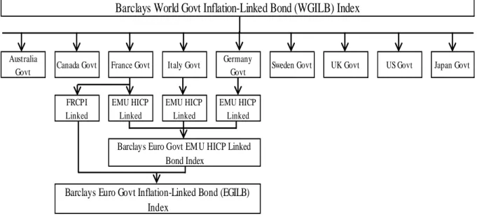
Figure 11: World Government Inflation-Linked Bond Index Structure………...…….26
Figure 12: EGILB Market Capitalization Weights………..………27
Figure 13: World Government Inflation-Linked Bond Index Structure………..……27
Figure 14: Inflation Evolution in the Considered Countries Year over Year (YoY)………...28
Figure 15: Graphical Relation between Nominal, Real and Breakeven Inflation Rates…..…34
Figure 16: Efficient Frontier Illustration……….………...………..37
Figure 17: Efficient Frontier, France………47
Figure 18: Efficient Frontier, Germany………...……….48
VII
INDEX OF EQUATIONS
Equation 1: Index Ratio………....22
Equation 2: Total Return Index………25
Equation 3: Consumers Price Index……….28
Equation 4: Fisher Equation……….33
VIII
GLOSSARY
BEIR – Breakeven Inflation Rate BTP – Buoni del Tesoro Poliennali BUND/OBL –Bundesobligationen CPI – Consumer Prices Index
EGILB – Barclays Euro Government Inflation-Linked Bonds Index ECB – European Central Bank
EUR – Euro currency
EMU – European Monetary Union GBP – Great Britain Pound currency GOVIE – Nominal Government Bond
HICP – Harmonized Index of Consumer Prices ILB – Inflation-Linked Bond
JGB – Japanese Government Bond MoM – Month over Month
NTN – Notas do Tesouro Nacional
OAT – Obligation Assimilables du Tresor SPGB – Spanish Government Bond
TIPS – Treasury Inflation Protected Treasuries USD – United States Dollar currency
WGILB – Barclays World Government Inflation-Linked Bond Index YoY – Year over Year
1
1. INTRODUCTION
Inflation-Linked Bonds (ILBs), have a recent history in the financial markets. Although there is evidence showing the early creation of these products back in the middle of the XVIII century, it was not until 1981 that they first appeared in Europe in the United Kingdom (UK). An introduction on how ILBs were first created as well as how they function will compose the initial part of the thesis, being this a structural chapter and thus introducing the specificities of these securities grounding the questions and tests assessed later on.
Recently, inflation has been a mainstream topic in Finance and Economics as Europe is facing a period of low inflation similar to the one faced by Japan since the 1990s, and threatening the economic recovery following the sovereign debt crisis of 2010. Hence, it is important to assess the role of linkers in today’s financial markets as well as from a portfolio management point of view. Apart from introducing linkers, conclusions on how they behave when faced with the risk/reward binomial relation and the benefits from including these securities in a portfolio are the basis originator of this dissertation.
ILBs are a relatively recent asset class where the first country to introduce these securities to the market was the UK with indexed-linked Gilts in the 1980s and the most liquid ILBs. United States of America (US) Treasury Inflation Protected Securities (TIPS), were only first issued in January 1997. The body of research is still considerably small when compared with other asset classes and with studies of relevance starting to be published in the latter years of the twentieth century. Campbell, Shiller and Viceira (2009) have studied, from a broader point, the history of ILBs in the US – TIPS – and UK – Gilts – relating and addressing yield levels, covariance and volatility with equities and bond supplies. Their main conclusions were related with the effect of long and short term real interest rates on ILBs yields. They also approached the evolution of these yields and justified the observed decrease in the period from 2000 to 2008 with an equal decreasing trend in the short term real interest rates, and then in 2008 in the peak of the US financial crisis, the sudden spike in ILBs yields was mainly due to the extreme market conditions causing a liquidity problem which led to the change in yields.
TIPS represent the ILBs subject to the most of the research due to the fact that they are more liquid and the US market for these instruments is considerably bigger. The majority of the research is related with the diversification benefits of ILBs from an asset allocation and investment perspective. Both Roll (2004) and Kothari and Shanken (2004) produced empirical
2 evidence that the inclusion of TIPS in a portfolio would enhance the diversification benefits in a portfolio composed by equities and nominal bonds. Later, Hunter and Simon (2005), by analyzing the real return betas of TIPS and the Sharpe ratios of both TIPS and the conventional nominal bonds concluded, that the primer showed evidence of superior volatility-adjusted returns.
However, as the ILB market increased in liquidity and as inflation expectations became more stable, and hence as the market matured, some studies, like the one developed by Brière and Signori (2009), showed that these factors contributed to the exponential increase in correlations with nominal bonds, therefore reducing the diversification benefits from 2003 on.
Currently, the benefits of ILBs are more closely related to inflation risk hedging benefits as demonstrated by Bekaert and Wang (2010) that by estimating and analyzing inflation betas1 for equities and nominal bonds concluded that ILBs were a key instrument to hedge inflation risk. This is a type of risk with which numerous investors face as they have liabilities directly related to changes in inflation or wages.
The body of research on the Euro area developed countries’ Inflation Linked Bonds is not very extensive. Hence this thesis intends to further analyze and extend the previous studies to the European Market by developing an analysis on the biggest issuers: Germany (Bundei/OBLei), France (OATei/i) and Italy (BTPei). Spain has also recently (last June), issued its first inflation linked bond the SPGBei 2024. However, since the data is scarce and very limited Spanish ILBs will be excluded from this study. Poland has also issued inflation linked debt securities. Yet by not having as much liquidity as the previous along with the focal point of this paper being to assess the properties of matured and developed markets including Poland might result in biased conclusions.
The main purpose of this dissertation is to introduce this new asset class that has recently been gaining notoriety. To do so the question that serves as cornerstone is: How have Euro area
developed countries’ ILBs evolved since they first appear, how do they function and best serve investors amid Portfolio Management? To get to a solid conclusion other sub questions will be
addressed:
1 As defined and computed by Bekaert and Wang (2010) the inflation betas define inflation hedging as how a
security‘s nominal return relates to with inflation in terms of covariance resulting in the following regression: 𝑅𝑖𝑡 = 𝛼 + 𝛽𝜋𝑡+ 𝜀𝑡 , where 𝑅𝑖𝑡 is the monthly nominal return of stock i, 𝜋𝑖 is the monthly rate of inflation, and
3 1. What is the history of ILBs? Why were they created and how did they evolve? What are these instruments specificities? How do they work and what are breakeven rates? 2. How did the ILBs returns from the different countries considered behave in the past
decade?
3. How do ILBs provide a better diversification benefits when compared with the traditional asset classes as equities and nominal bonds and how well do they perform in this topic according to the efficient frontier theory?
The remainder of the thesis is organized as follows: Section 2 provides an overview on the relevant literature related with ILBs which intends to provide some contextualization on what can be expected on the conclusions of the empirical analysis. Section 3 is the cornerstone of this dissertation as it is the chapter that introduces the history behind ILBs. It starts by giving an overview of how linkers first appeared and then focus more on the Euro area market, divided by country. It can be expected to acquire relevant insights on the origin of linkers, how they work and how these instruments are structured. The following section 4 details the data used in the present thesis, explaining the source of data and how Barclays Capital indices are used to study on ILBs’ diversification power and asset allocation. Section 5 consists in presenting the descriptive statistics on all the data used in this study where the objective is to introduce the empirical analysis and the methodology used in the rest of the dissertation. The next section 6 is on the methodology used to access the proposed questions. There are presented in this chapter some well-known financial concepts and theories as the Fisher Equation and Markowitz’s efficient frontier which will be later on addressed. Section 7 focus on the diversifying power of ILBs through the analysis of correlations with inflation, between asset class and cross-country. Asset allocation in section 8 is the one that concludes the empirical analysis and focus on optimizing a portfolio using equities, nominal sovereign bonds and linkers trough the efficient frontier framework as well as opposing portfolios composed by equites and ILBs and equites and govies then accessing the returns, volatility and Sharpe ratios. Concluding the study we have section 9 which summarizes the dissertation, provides the main conclusions and offers answers to the above mentioned questions by giving investor advices and guidelines on inflation-linked bonds.
4
2. LITERATURE REVIEW
ILBs have been addressed and researched in the past. Essentially in the past 20 years, several acknowledgeable authors have studied these instruments where the general focus was related with their diversification benefits and from a comparable point of view against nominal bonds. The focus here will be on papers which address ILBs of developed and matured markets, describing the behavior and specific characteristics, as volatility and correlation, of ILB among the financial markets. Therefore, an outline of the most relevant research of the matter is presented allowing the reader to pace himself along with the existing studies.
This chapter is divided in two sub sections as it is intended to separate the main findings regarding the correlations and volatilities conclusions from others regarding portfolio allocation and efficiency. Although correlations and volatility will affect and serve as the basis for an analysis regarding portfolio allocation, the aim here is to also set apart other conclusions such as price and yields discrepancies, duration, trends and inflation hedging properties.
2.1. Correlations and volatility
Roll (2004) took an empirical approach on the US ILB market (TIPS) and tried to infer on their specific characteristics and behavior. The author collected a sample of data of these instruments from July 1997 to August 2002. The first conclusion was on the correlation where TIPS returns were highly correlated to each other, mainly within similar maturities. Secondly, the volatility of TIPS was rather small between 1999 and 2000 and increased by a great deal after 2000. The correlation of TIPS returns with other assets was seen as positively related to nominal bonds and inversely correlated with equities.
Kothari and Shanken (2004) simulated hypothetical ILBs returns using historical yields of nominal US Treasury Bonds and an inflation forecasting model. They concluded that ILBs were less volatile than the equivalent nominal bonds and that the correlation with equities was considerably lower due to the inflation protection effect.
Hunter and Simon (2005) addressed the correlation between TIPS and nominal bonds. To do so, they collected weekly data from February 1997 to August 2001, and used a multivariate
5 GARCH model2 to estimate the time-varying correlations. The conclusions led to an interesting finding. The results showed that the real rate components tended to increase with time which produced lower TIPS returns. Moreover they concluded that an increase in TIPS returns was always preceded by an increase in nominal yields returns, showing that nominal yield returns lead TIPS returns. In the case of a flatter (steeper) yield curve, there is an associated higher (lower) conditional correlation of returns within a confidence level of 5%. Also, the spreads have shown to have an effect on correlation as at the 1% confidence level; an increase in the spreads between Treasuries and TIPS often is allied with higher correlation. Besides from the analysis made on TIPS regarding their correlation with nominal bonds, Hunter and Simon (2005) also approached TIPS from the risk/benefit binomial relationship and through the analysis of volatility they computed Sharpe ratios and conditional real betas which led them to conclude that TIPS showed evidence of higher volatility when compared with nominal bonds, particularly in times of superior inflation expectations.
Brière and Signori (2009) started their research on the diversifying power of ILBs using daily returns from a sampling period from 1997 to 2007. They focused on three asset classes in US and Europe (EU). For ILBs they used the Barclays Global Inflation Total Return indices for US and the French Linkers for EU. The nominal bonds were represented by Barclays Breakeven Comparator Bond indices for both US and EU and finally for Equities the authors used the S&P500 for US and the DJ Euro Stocx for EU. The results of their on the conditional correlations and volatilities between the referred asset classes indicated that in more recent times, mainly from 2003 and further, with higher liquidity in the linkers market along with stable inflation expectations, ILBs and nominal bonds both in the US and EU were almost substitutable assets. The main conclusion was that the higher correlation verified indicates similar volatility between the inflation protected bonds and the nominal equivalents, hence eliminating in most ways the diversification power that ILBs had in the past.
Campbell, Shiller and Viceira (2009) developed their research on ILBs based on data from the UK and US (these are the two largest and recognized ILBs markets). The authors analyzed several factors such as volatility, correlations, and the level of yields and the supply of these securities. The results on TIPS and inflation-indexed Gilts showed that there was a huge
2 Generalized Auto Regressive Conditional Heteroskedasticity (GARCH) model developed by Engle (1982) is an
econometric process used to estimate volatility in financial markets. It starts by estimating the best-fitting autoregressive model then computing autocorrelations of the error term and finally testing for significance.
6 decrease in long-term real interest rates from 1990 to 2008 when in the beginning of the financial crisis there was an abrupt increase, which was later concluded to have its cause on the liquidity problems that raised then and created inexorable market discrepancies. The breakeven inflation rates sooth until 2008 after when they showed striking decreases.
2.2. Portfolio allocation
Roll’s (2004) main conclusion was related with the duration which due to the low real yield of TIPS was longer than the comparable nominal peers. However, when a daily analysis was conducted the author concluded that TIPS duration was less volatile due to the impact of changes of expect inflation being lower. Finally, Roll concluded that the Nominal Bond’s yields reflected the expected inflation whereas TIPS did not. Based on this, adding inflation to the TIPS real yields would make them look more attractive as higher the inflation, being this the reason Roll used to justify the downturn in TIPS real yields in 2002; lower inflation expectations.
Based on the findings with regard to both the lower ILB’s volatility with the nominal comparables and lower correlations with equities, Kothari and Shanken (2004) stated that ILBs provide additional diversification benefits when included in a portfolio composed by bonds and equities. The low correlation and volatility resulted in lower standard deviation of an equal-weighed portfolio of stocks and bonds when ILBs replaced the nominal and conventional equivalents. These findings were the base line in the authors’ opinion on the importance and benefits of ILBs in investor’s asset allocation decisions since Kothari and Shanken stated that investors depend on the expected return and risk of the available asset classes. Finally, they vowed that the fact that TIPS were a market with limited liquidity increased their yields, hence making them a more attractive investment in a long-term investment horizon period as was later supported with an analysis of TIPS actual returns from February 1997 to July 2003. Hunter and Simon (2005) also presented results concerning the diversification benefits on including TIPS on a portfolio and concluded that the benefits differed for each portfolio according to their specific characteristics. During times of constant inflation rates, adding TIPS to a portfolio with other nominal bonds would increase considerably the risk-rewards benefits. Conversely, in the presence of a more diversified portfolio that would include nominal Treasuries, the benefits would be close to null. Yet, during high inflation periods linkers would still play a major contribute in increasing the portfolio efficiency regardless of the level of
7 diversification of the existing portfolio. Relating with Roll (2004), a similar suggestion was made, stating that during times of high expected inflation, adding TIPS to a portfolio of equities and nominal bonds would improve the portfolio efficiency.
Apart from the diversification analysis, Brière and Signori (2009) also approached the ILBs benefits by studying monthly dynamic portfolio optimization based on the previous computed estimates on volatility and conditional correlations. Again, the results indicated that although ILBs showed diversification benefits in portfolio asset allocation in developed countries before 2003, this effect was now mitigated and the weight in the optimal portfolio decreased exponentially. This decrease was more notable in the EU case where ILBs weight was close to nothing. This conclusion supports the same thesis presented before and simply comes to a point where the inclusion of ILBs in a portfolio nowadays resumes itself to the investors’ inflation risk aversion and their consequent expected returns when compared with nominal bonds. Campbell, Shiller and Viceira (2009) tried to explain the trends before 2008 when it came to short-term interest rates, liquidity and bond risks. Firstly, they re-ran the VaR analysis of Campbell and Shiller (1996) on the expectations hypothesis of the term structure of ILBs. They provided conclusions on the behavior of yields and their decrease from the beginning of the twenty first century and forth, that were greatly explained by the low levels of real interest rates. The asset pricing theory3 was used to estimate a model of pricing from Campbell, Sunderam and Viceira (2009), with a time-varying systematic risk and concluded that the covariance between TIPS and equities has a strong effect on TIPS yields with strong and persistent risk variations.
Bekaert and Wang (2010) developed their research on Gilts, TIPS and Euro area ILBs. The authors based their work on old academic papers to conclude on ILBs pros and cons. The main benefits were the support of market completeness and efficiency mainly in the distribution of risk; also they contributed to savings in government’s debt costs, the reduction in government inflation measures and finally giving information on inflation expectations and real interest rates. However, the authors described weaknesses of the theoretical benefits, such as the size and liquidity of this market, mainly in the beginning years of TIPS.
3The asset pricing theory states that the expected return of a financial asset can be modeled as a linear function of
various macroeconomic factors or theoretical market indices represented by a factor-specific beta coefficient. Here the authors used it to assess ILB’s risk premium where they first started from a consumption based pricing model and then simplified it to a more empirical and less structural analysis based on changes of covariance between bonds and stocks.
8 Bekaert and Wang (2010) also approached the benefits of ILBs from another fundamental point of view: inflation risk hedging. Using a sample period between January 1970 and January 2010 (depending from country to country) and composed by data from countries, they estimated inflation betas for nominal sovereign bonds and equities. The results, both for short and long term investment horizons, showed that in half of the countries bond returns were inversely correlated with inflation and that equities did not provide hedging for inflation. Therefore, the authors stated that ILBs would be a crucial security to hedge inflation as they incorporated a better capacity of measuring inflation risk premium to investors.
9
3. HISTORICAL OVERVIEW
This chapter has as its main objective the introduction of ILBs through an overview of its history. Here it will be presented when, how, why and where these instruments were first created and issued as well as how they work in terms of its nominal and coupon payments. As this dissertation focus on the European developed market, a focus will be set on the issuers mentioned before: Germany, France and Italy.
It is important to provide the reader with this information and contextualization so that a further comprehension of the study is allowed and of easier understanding, as the main purpose here is to give notice of ILBs and their role in current financial markets.
Investment returns can be highly conditioned by inflation, as this macroeconomic factor can cut deeply into portfolio’s returns if not considered and properly assessed its risk. Let us assume we are a portfolio manager working in Europe and during the year of 2014 we achieved an overall portfolio return of 10%, considering the ECB inflation target of close to 2%. In the event of a poor inflation analysis and hedging, the portfolio would see its returns diminished by 20%. ILBs would come to play its part here, as these instruments can help to offset and hedge inflation risk as they increase in value during inflationary periods.
Although inflation has not been a major economic factor in the recent past it is now gaining notoriety. ILBs markets have been developing fast and these fixed income securities are more and more seen as an instrument to reduce future uncertainty and hedging inflation, becoming a popular long-range planning investment vehicle both to institutional and individual investors.
3.1. The Origin of Linkers
ILBs go back to the 18th century when they were first issued to fight the corrosive impact of inflation on the real value of consumer goods during times of rise in prices. The Massachusetts Bay Company was the first company to issue this type of bonds, beginning in the 1780s with money market securities, indexing their bonds to the price of silver and other items, thus reflecting inflation. However, at the time the issue did not achieve the expected success as few investors were interested in it. On the other hand side, after the exponential economic growth following World War II, sovereign and governmental financial planners started to look to the possibility of using these securities. In the 1950s we saw the first capital markets ILBs issuing
10 with Israel and Iceland that at the time aimed at fighting high inflation due to their rapid growth in GDP.
The first big issuing of ILBs happened in the 1980s and this was the moment that marked the birth of modern inflation-linked bond market which happened by the hands of United Kingdom, more precisely in 1981. This was followed by Australia in 1985, Canada in 1991, and Sweden in 1994, the United States reentered the market in 1997 with its famous TIPS, France in 1998 which bonds were linked to the French inflation (OATi) and Euro-zone inflation (OATie). Italy in 2003 as well as Greece entered the euro area linker market, Japan in 2004 (in spite of its deflationary environment), Germany in 2006 and most recently Spain issued its first inflation-linked debt security in 2014.
According to Barclays Inflation Indices, this market has been growing significantly in the past 10 years, where the WGILB index has grown about 400% in market value from about €381 billion in January 2004 to close to €2 trillion in 2014, going from having 39 bonds to 114. This increase is analogous to the evolution around the globe as shown in figure 1, where the biggest increase happened in Japan and in the Emerging Markets Government Inflation-Linked Bond (EMGILB) index with a rise of about 4000 and 2600 percent respectively in terms of market value. In the most developed countries the increase was also notable, however much more modest when compared with the two mentioned before. The EGILB index grew about 250% from €80.42bn to about €280bn in the 10 year period. In US and UK the market capitalization of linkers went from €183bn to €893bn in the first and a growth of €486bn in the second, from €129bn in January 2004 to €616bn in December 2014.
This growth had big influences in the dynamics of the inflation-linked bond market. As observed by Brière and Signori (2009), the increase in liquidity from 2003 and afterwards combined with other factors as stable inflation expectations, contributed to a increase in correlations and similar volatility between linkers and nominal bonds in the most developed markets, mainly in the US and Europe, concluding that the two asset classes were now almost substitutes. This reduced the role of linkers to inflation protection properties and financial planning. While this last point was stated by Bekaert and Wang (2010) as one of ILBs main benefits as they contribute to savings in government’s debt costs, the reduction in government inflation measures and finally giving information on inflation expectations and real interest rates.
11
Figure 1: ILBs Indices Evolution by Market Value in Euros
Source: Barclays Capital
Other countries have also issued ILBs, mainly in Emerging Markets (EM) like Brazil, Turkey, South Africa and Mexico; however, these countries having a poor credit rating while others due to their small size and lack of liquidity are impeded of entering the major and most broadly used indices. An interesting fact occurred in some of these EM countries as at some stages, these countries could only issue ILBs since due to their weak currencies and persistent high inflation, investors would not buy nominal assets of these same countries. Brazil is currently the bigger issuer of linkers within the EM countries category, representing a large portion of this market, with over $300 billion in market value outstanding and dating its first issue back to 1964.
3.2. European Inflation-Linked Bonds
The history of European ILBs is undeniably interconnected with the birth of the HICP index in 1996 by Eurostat, the agency responsible for creating and managing common consumer price indices in Europe. This index also known as the Monetary Union Index of Consumer Prices (MUICP), serves as reference for the ECB within its monetary policy actions in order to fulfill its mandate of price stability with the index close but below 2%.
France was the first sovereign issuer from the euro area which presented its linkers in 1998 with the OATi 3% Jul 2009, at the time linked to the French CPIx. However, before that some inflation derivatives such as inflation swaps were already trading in the secondary markets and
0 500,000 1,000,000 1,500,000 2,000,000 2,500,000 20 04 20 05 20 06 20 07 20 08 20 09 20 10 20 11 20 12 20 13 20 14 Ma rk et Valu e (E u r M)
12 indexed to the MUICP. Later in 2003 the Italian Government issued its first linker which was indexed to the HICPx as most Italian inflation liabilities also exclude tobacco and then confirming this as the benchmark index for both inflation-linked bonds and derivatives in the euro area.
Nowadays both HICP indices and CPI indices are computed via geometric chain weighted Laspeyres4 indices with annual indexation reviews at the beginning of each year which aims to adjust and reflect consumption weights changes amid countries. The final MUICP is normally released around the 17th of the following month, however every month end it is released a flash estimate, with data collected from each individual country, which is then revised and adjusted if needed, hence reducing the uncertainty in the final inflation releases.
In 2006 Germany entered the ILB market, although the announcement was made in 2004, which then marked the inclusion of all G7 countries in the linkers market.
Greece, which in spite of being excluded from this dissertation and analysis, was the second euro area government to issued HICPx linked bonds in March 2003. Previous to that and joining the monetary union, Greece had also other small issues of bonds linked to the domestic CPI which matured in 2007.
Finally, Spain closed the euro area linker market with two issues in 2014. Both ILBs, a 5y and 10y references, where extremely successful which now puts Spain in a steady pace to becoming another large issuer of inflation-linked debt securities.
France
France first announced its intention to issue ILBs on December 3rd 1997 which was then effective on the 15th of December 1998 with the issue of the OATi 3% Jul 2009 via syndication with several re-openings by auction. As noted before, the index was then decided to be the one released by the French NSA (Institut national de la statistique et des études économiques – INSEE), with the official measure of French consumer prices, the CPI excluding tobacco. Although this index would best serve the interest of the government, as it would be a more accurate measure of the domestic price evolution and liabilities, investors soon started to demand a broader European measure. Yet the Eurostat HICP had been recently created and
4 The Laspeyres price index measures the price development of a basket of goods and services consumed in a base
13 still with some disadvantages, as lack of track records, partial index coverage in some countries and the tests on the index were not carried to the desired full exhaustive amount with some fears of significant revision adjustments.
Another fact that may be considered a coincidence was the fact of the first ILB issue timing concurrence with the beginning of the European Monetary Union (EMU). This was in fact a key consideration for the French authorities as this event was expected to drive the intensity, competition and liquidity in the European sovereign fixed income financing market. Hence France was looking for gaining advantage by being the first to issue inflation-linked bonds. The OATi 3.4% Jul 2029 marked the second tapper of the French Government one year later in September 1999, once again linked to the national CPIx. The issuing followed the same steps of the previous one with an initial syndication with some occasional later re-openings. The growth in the outstanding value of the two issues showed a slow but steady pace which cause some worries regarding to the capture of euro area investors interest outside France. Later in October 2001, France determined to change the weak outstanding growth launching the first issue linked to the HICPx through syndication and exchanges out of the OATi Jul 2009. As there were some concerns considering the liquidity impact in the remaining linkers this proved not to be the case as this later issuing gave a lot of momentum to the French ILBs (figure 2), and to the sector as a whole, reflected in daily turnovers, making France the number one issuer in terms of outstanding amount by market value in the euro area with close to €206bn.
Figure 2: Evolution of the French ILB Market by Market Value
Source: Barclays Capital 50,000 100,000 150,000 200,000 250,000 20 04 20 04 20 05 20 05 20 06 20 06 20 07 20 07 20 08 20 08 20 09 20 09 20 10 20 10 20 11 20 11 20 12 20 12 20 13 20 13 20 14 20 14 Ma rk et Valu e (E u r M)
14 After the noted increase in the interest in the linkers markets, France responded by quickly picking-up the supply. The responsible treasury French agency (Agence France Trésor – AFT) has been increasing ILB issuance with issuances occurring almost every month.
According to figure 3, ILB have had a good performance in the analyzed period with returns on average5 around 4.87% while the nominal government equivalent averaged 5.3% and the equities with approximately 4.19%. When we also considered the average annual standard deviation and compute the ratio between the first and the annual returns we can see that the nominal bonds rank first with a value of 1.34, followed by the ILBs with 0.94 and lastly equities with 0.2. However, this last category was highly influenced by the financial turmoil starting in 2008 with the crisis in the US. These numbers suggest that in the French case, the investor, when deciding accordingly to the risk/return binominal relation would be better of investing in sovereign nominal bonds.
Figure 3: French Market – Historical Performance and Risk
Source: Author’s calculation based on Barclays Capital
Germany
In Germany, the beginning of the inflation-linked market happened in March 2006 in spite of the announcement being made much earlier by the German officials in 2004. The Bund which had as a reference index the HICPx was issued with a maturity of 10 years, a coupon of 1.5% and with initial size of €5.5bn via syndication. The objective was to increment the size of this
5 The computed averages are all average annualized returns.
0% 5% 10% 15% 20% 25% 30% 35% 40% 45% -60% -50% -40% -30% -20% -10% 0% 10% 20% 30% 2004 2005 2006 2007 2008 2009 2010 2011 2012 2013 2014
ILB Govt Equites
15 same issue in later re-openings which did in fact happened in September 2006 (€3.5bn) via syndication and later switched to an auction mode tapering. In October 2007 the OBLei 2.25% April 2013 was issued and in June 2009 Germany decided to launch another linker, the Bundei 2020, which was the first one after the exponential deflationary decrease in inflation breakevens during the second semester of 2008.
The German development of its inflation-linked bond curve had been slower than previously anticipated and the Bundei 2020 came to reassure the linker market the commitment of the country. Later on the taper adopted a more steady pace although still quite moderate as seen in figure 4, with issues in April 2011 (OBLei 2018) and in March 2012 (DBRei 2023), with amounts circling between €8 to 12bn. In 2014 there were over 11 auctions totaling €17.2bn with a bid-to-cover ratio6 of 1.8 making Germany, as of December 2014, the third larger issuer of ILBs in the euro area with approximately €74.6bn outstanding (market value).
Figure 4: Evolution of the German ILB Market by Market Value
Source: Barclays Capital
Germany ILBs have had a similar behavior when related with the French equivalents, showing since its inception an average return of 3.7%. The nominal government bonds and the equities had returns around 4.8% and 9.26% respectively as showed in figure 5, with equities showing more than 6 times the return when compared with the French equities. Both in France and
6 The bid-to-cover ratio compares the number of bids received in a Treasury security auction to the number of
bids accepted therefore signaling the strength of the demand. A ration above 2 represents a successful auction with aggressive bids while a number below 1 shows a disappointing auction and wider bid-ask spreads.
10,000 20,000 30,000 40,000 50,000 60,000 70,000 80,000 20 06 20 07 20 08 20 09 20 10 20 11 20 12 20 13 20 14 Ma rk et Valu e (E u r M)
16 Germany, the government bonds act many times as refuge/safe investments due to these countries high credit ratings, more preeminently during stress periods, which lead one to think about their correlation being, theoretically, close to 1, potentially reducing their diversification benefits when included in an efficient portfolio.
When considering the standard deviation of the returns, we see that the nominal government bonds were the asset class that best behaved with a value around 1.16, followed by the linkers with 0.95 and finally equities with 0.43. It is important to mention that these results are heavily affected by the financial crises and the subsequent raise in volatility in the markets with due to the higher risk in equities is much more pronounced in this type of securities.
Figure 5: German Market – Historical Performance and Risk
Source: Author’s calculations based on Barclays Capital
Italy
Italy first announced its intention to issue ILBs on September 2003 and after just five days took many by surprise by syndicating its first linker, a €7bn BTPei September 2008. Although this struck the market unprepared the issue was a success and was quickly embraced and accepted among all market participants which allowed a re-opening one month later increasing the outstanding amount issued to a little over €10bn.
This bond, like the conventional BTPs, paid a semiannual coupon and was priced via interpolation spread to the nominal curve. However, due to the tapering of the Italian Government of nominal bonds the following week with a matching maturity to the linker some breakeven trading took place, further enhancing the issue liquidity.
0% 5% 10% 15% 20% 25% 30% 35% 40% 45% -50% -40% -30% -20% -10% 0% 10% 20% 30% 40% 2006 2007 2008 2009 2010 2011 2012 2013 2014
ILB Govt Equities
17 The Italian domestic demand for inflation-linked notes was high, however since there was not any 5y point in the French OATei (at the time the European-Inflation linked bonds reference curve), it was relatively difficult to investors to take positions in that maturity that until then were using structured products. This was the fact that served as basis for the choice of the maturity of the first BTPei, boosting demand and liquidity and assuring a successful launch of Italian linkers.
After the opportunistic 5y linker the next bond aimed to a longer maturity: the 10y BTPei 2.15% September 2014, which was placed initially through syndication and later via auctions going on to an outstanding close to €14.5bn. In the subsequent years Italy launched other ILBs starting the construction of its inflation-linked bond yield curve with bonds maturing up to 30 years.
March 2007 marked the first Italian linker issued and placed through auction leaving the syndication back with the BTPei 2012. Yet, the Italian Treasury went back to the syndication in June of the same year when it launched the BTPei 2023, their first 15y linker. Another issue that marks the history of ILBs in Italy was the private placement of two ultra-long dated bonds, with smaller amounts, maturing in September 2057 and 2062 that also motivated some extra activity in the ultra-long inflation linked swaps market.
2005 was also an important year for the Italian linker market as it surpassed France as the country with the higher number of bonds linked to the euro HICPx. The years of 2008 and 2009, due to the financial crises, reduced the number of ILBs issuances, in all euro area countries alike, with even issues being canceled. However, after these years, the issuance pace got back to a steady and growing pace with the Italian government issuing several bonds in the next couple of years. In spite of that, in 2012 in the height of the financial crisis in Europe, the Italian fixed income market suffered tremendously, much like other peripheral European countries, which culminated in the decision of including nominal bonds in the ECB securities market programme (SMP). The fact the the ILBs were excluded from the programme originated several discrepancies in terms of breakeven valuations which lead to a significant sell off in the linkers, as seen in figure 6, and pushing real yields very high without ECB to absorb the selling streak. The Italian authorities tried to balance the ILB market by conducting buybacks and switch auctions out of BTPei, but the public debt issuance agenda for 2012 indicated that the supply would likely fall due to some issues maturing but the Italian treasury
18 rescheduled the linkers taper so it could give them more room to maneuver the linkers issuance without creating too much of externalities and discrepancies in the market.
Figure 6: Evolution of the Italian ILB Market by Market Value
Source: Barclays Capital
Italy introduced to the market a new inflation-linked product in March 2012. This bond was intended to the domestic retail investors as it had as reference the Italian Famiglie di Operai e
Impiegati (FOI) inflation excluding tobacco, which is an index that represents a basket of
consumption goods of household’s workers. This linker, maturing in 2016, was open to both institutional and individual investor during four days in an amount close to €7.3bn, where they could get access via banks or internet. The coupon was fixed in the end of the four days with a minimum of 2.25%. Later on the statistics revealed by the Italian Treasury showed that most of the bonds were sold in contracts over €50,000 which is commonly used as an indicator to distinguish between individual and institutional investors.
When analyzing the performance from the different asset classes presented in figure 7, we see that the returns of ILBs where quite similar to the ones of the nominal government equivalents as observed in France and Germany, with only 0.6% separating the two, 5.2% and 5.8% respectively, during the 10 year period from 2004 to 2014. The equities, on the other hand, suffered a much worse devaluation during the financial crisis and therefore have a negative return of -0.15%. Again, when dividing the returns by the standard deviation we observe the same ranking between the three asset classes with the nominal government bonds placing first with 1.1 followed by the linkers 0.74 and finally the equities with -0.007. Interestingly enough
0 20,000 40,000 60,000 80,000 100,000 120,000 140,000 160,000 20 04 20 04 20 05 20 05 20 06 20 06 20 07 20 07 20 08 20 08 20 09 20 09 20 10 20 10 20 11 20 11 20 12 20 12 20 13 20 13 20 14 20 14 Ma rk et Valu e (E u r M)
19 is that in Italy the difference in this ratio is not as pronounced as it happened in both France and Germany, suggesting a higher correlation of returns and hence the substitutability between these two assets as suggested by Brière and Signori (2009).
Figure 7: Italian Market – Historical Performance and Risk
Source: Author’s calculations based on Barclays Capital
Others
There are some other countries within the euro area who have also issued ILBs. Although they are mentioned here, they are not included in the quantitative analysis of this dissertation for reasons such as lower liquidity, credit quality, low outstanding or because there are simply too recent as in the case of Spain.
Starting with Greece, this ancient country had issued ILBs before it even entered the euro area. These bonds were linked to the Greek CPI and in small amounts having the last of these linkers matured in 2007. Although Greece ILBs are not included in the quantitative analysis they are part of the European linker market history as they were the second country to have issued a euro HICPx linked bond, the GGBei 2.9% Jul 2025 via syndication during Mach 2003.In March 2007 a new reference in the Greek inflation-linked curve was launched with the GGBei 2.3% July 2030 having the Greek Treasury also addressed the ultra-long-date market via private placement with a bond with maturity up to 50 years at the same time and once again in 2012. 0% 5% 10% 15% 20% 25% 30% 35% 40% 45% -65% -45% -25% -5% 15% 35% 20 04 20 05 20 06 20 07 20 08 20 09 20 10 20 11 20 12 20 13 20 14
ILB Govt Soma
20 Greek ILBs were also subject to the same binding program as the nominal bonds which, similar to the Italian comparators, created heavy discrepancies in this market and today there are no Greek ILBs on the market.
Much more recently and after months of studies and careful research, the Spanish authorities decided in May 2014 to launch its first HICPx ILB, a 10y reference of up to €5bn. The year of 2014 was a great year for fixed income securities in Europe as since 2013 there was a strong and consistent bull market after the peak in yields in 2012 when the financial sovereign debt crisis hit the strongest level in Europe. This fact, which leads to a confidence increase in investors and consequently successful nominal issuances, with high bid-to-cover ratios and lower financing costs, paved the way for the first Spanish linker.
The timing was not the best in the point of view of investors as this was a period of low inflation expectations, which as studied by Roll (2004) was proven to drive down the real yields and push the prices upwards. However, Spain’s objective was to assume the interest in issuing ILBs and entering the market then joining France, Germany and Italy, capturing a broader share of investors.
Still during 2014 Spain issued its second ILB, this time the bond had a maturity of 5 years in order to start constructing its inflation yield curve.
3.3. How do Linkers work?
Inflation-linked bonds have as their main objective the protection of investor’s purchasing power over their investments. There is one main difference in ILBs when compared with nominal bonds: the principal/nominal and coupons value, which in the first is variable and depends on the value of the underlying inflation index (figure 8).
21
Figure 8: Comparison between Nominal and Inflation-Linked Bonds’ Structure
Source: Author’s illustration
In short, in the nominal conventional bonds there is a nominal fixed coupon and redemption payment agreed at the issuance, including inflation expectations at the time. However, they are not adjusted during the life of the bond. By contrast, linkers are adjusted accordingly to the realized inflation in one of two ways:
1. The coupons are adjusted in line with inflation and the redemption remains constant; 2. The redemption value is indexed, continually, to inflation and the coupons are set as
fixed, varying with the nominal redemption value.
The second method is the most commonly used in ILBs around the world and is illustrated in figure 9.
Figure 9: Illustration of ILBs’ Principal and Coupon Mechanics
Source: Author’s modifications based on Pacific Investment Management Company
Nominal Bond ILB
F ixe d nom ina l c oupon w it hout a dj us tm ent s F ixe d re al c oupons w ith infl ati on a dj us tm ent s
22 The nominal face amount, thus the repayment of principal, and consequently the fixed coupons of ILBs are computed by taking into account the variations in the real quantities based on the variation of the inflation rate. A ratio is computed from the reference inflation index on every coupon date or principal repayment date and the reference inflation rate at the time of the linker issuance date: the Index Ratio; which is then multiplied by the values excluding inflation.
𝐼𝑛𝑑𝑒𝑥 𝑅𝑎𝑡𝑖𝑜 =𝑃𝑟𝑖𝑐𝑒 𝐼𝑛𝑑𝑒𝑥𝑐𝑢𝑟𝑟𝑒𝑛𝑡
𝑃𝑟𝑖𝑐𝑒 𝐼𝑛𝑑𝑒𝑥𝑡=0 (1)
As presented above, it is seen that the inflation index is the ratio that underlies any linker. To better understand the differences between an ILB and a nominal equivalent it is presented bellow an example opposing a 10y traditional bond (N) and an equivalent ILB. Both securities have a nominal value of €1,000.00, while for the linker it is assumed a real coupon of 2% and a constant inflation rate of 2% over the 10 year period until the maturity of the bonds. The nominal bond is assumed to have a coupon of 4.04% in order to match its expected real income to the real coupon of the linker:
𝐸𝑥𝑝𝑒𝑐𝑡𝑒𝑑 𝑟𝑒𝑎𝑙 𝑟𝑎𝑡𝑒 𝑜𝑓 𝑟𝑒𝑡𝑢𝑟𝑛𝑁= (1 + 𝐶𝑜𝑢𝑝𝑜𝑛𝐼𝐿𝐵) ∗ (1 + 𝑖𝑛𝑓𝑙𝑎𝑡𝑖𝑜𝑛 𝑟𝑎𝑡𝑒) − 1 𝐸𝑥𝑝𝑒𝑐𝑡𝑒𝑑 𝑟𝑒𝑎𝑙 𝑟𝑎𝑡𝑒 𝑜𝑓 𝑟𝑒𝑡𝑢𝑟𝑛𝑠 𝑁 = (1 + 2%) ∗ (1 + 2%) − 1 = 4.04%.
In table 1 it is presented the structure of cash flows for each bond, both in real and nominal terms. In the traditional bond, both the nominal face value and the nominal coupon remain unaltered during the entire time period as with the real value of the payments falls with the inflation as it is discounted to t=0, therefore accounting for the loss of purchasing power. Hence, we can derive the real value of the nominal payment and the coupons by including the inflation index with:
𝑅𝑒𝑎𝑙 𝑉𝑎𝑙𝑢𝑒𝑡= 𝐹𝑎𝑐𝑒 𝑉𝑎𝑙𝑢𝑒 (1 + 𝑖𝑛𝑓𝑙𝑎𝑡𝑖𝑜𝑛)𝑡= 1,000 (1 + 2%)𝑡 and 𝑅𝑒𝑎𝑙 𝐶𝑜𝑢𝑝𝑜𝑛𝑡 = 𝐶𝑜𝑢𝑝𝑜𝑛 (1 + 𝑖𝑛𝑓𝑙𝑎𝑡𝑖𝑜𝑛)𝑡= 40.4 (1 + 2%)𝑡 .
In the ILB the values that remain unchanged are the real values of the principal and interest payments, where the variations happen in the nominal figures which vary over time with the inflation index:
23 𝑁𝑜𝑚𝑖𝑛𝑎𝑙 𝑉𝑎𝑙𝑢𝑒𝑡 = 𝐹𝑎𝑐𝑒 𝑉𝑎𝑙𝑢𝑒 ∗ (1 + 𝑖𝑛𝑓𝑙𝑎𝑡𝑖𝑜𝑛)𝑡 = 1,000 ∗ (1 + 2%)𝑡
and
𝑁𝑜𝑚𝑖𝑛𝑎𝑙 𝐶𝑜𝑢𝑝𝑜𝑛𝑡 = 𝐶𝑜𝑢𝑝𝑜𝑛 ∗ (1 + 𝑖𝑛𝑓𝑙𝑎𝑡𝑖𝑜𝑛)𝑡= 20 ∗ (1 + 2%)𝑡.
With respect to the inflation index, the point in time t value, assuming a base value of 100 at issuance, it is computed as in formula 1:
𝐼𝑛𝑑𝑒𝑥 𝑅𝑎𝑡𝑖𝑜𝑡 =
𝑃𝑟𝑖𝑐𝑒 𝐼𝑛𝑑𝑒𝑥𝑡 𝑃𝑟𝑖𝑐𝑒 𝐼𝑛𝑑𝑒𝑥𝑡=0=
100 ∗ (1 + 2%)𝑡 100
Table 1: Comparing Cash Flows between Traditional and Inflation-Linked Bonds
Source: Author’s calculations based on example from Wrase (1997)
It is possible to conclude from the observed above that ILB have as characteristics inflation adjusted nominal value, this is given to these securities having inflation index relationship while the traditional bonds have their nominal values constant over the bond’s life.
As shown by the total nominal receipts of both bonds, the smaller nominal interest payment during the life of the linkers is offset by a higher principal payment at maturity which reflects the 10 year inflationary period as illustrated in figure 10. In the traditional bond, although offering an equivalent real coupon at issuance, as it did not account for the inflation, resulted in lower nominal benefits at the maturity of the bonds. Looking through the Net Present Value
Euros
Year Nominal Value of Principal Real Value of Principal Nominal Interest Payment Real Value of Interest Payments Nominal Value of Principal Real Value of Principal Nominal Interest Payment Real Value of Interest Payments 1 1.000,00 980,39 40,40 39,61 1.020,00 1.000,00 20,40 20,00 2 1.000,00 961,17 40,40 38,83 1.040,40 1.000,00 20,81 20,00 3 1.000,00 942,32 40,40 38,07 1.061,21 1.000,00 21,22 20,00 4 1.000,00 923,85 40,40 37,32 1.082,43 1.000,00 21,65 20,00 5 1.000,00 905,73 40,40 36,59 1.104,08 1.000,00 22,08 20,00 6 1.000,00 887,97 40,40 35,87 1.126,16 1.000,00 22,52 20,00 7 1.000,00 870,56 40,40 35,17 1.148,69 1.000,00 22,97 20,00 8 1.000,00 853,49 40,40 34,48 1.171,66 1.000,00 23,43 20,00 9 1.000,00 836,76 40,40 33,80 1.195,09 1.000,00 23,90 20,00 10 1.000,00 820,35 40,40 33,14 1.218,99 1.000,00 24,38 20,00 Total Nominal Receipts 1.404,00 Total Nominal Receipts 1.442,37 Real value of principal at maturity 820,35 Real Value of Indexed principal at maturity 1.000,00
24 (NPV) approach in order to create a simple exercise, assuming a discount rate of 5%, we would be comparing a value of €390 for the linker and €312 for the traditional bond.
Figure 10: Cash Flow Structure of an ILB
Source: Author’s calculations based on example from Wrase (1997) 2.04% 2.08% 2.12% 2.16% 2.21% 2.25% 2.30% 2.34% 2.39% 2.44% 21.90% 100 105 110 115 120 125 0% 5% 10% 15% 20% 25% 1 2 3 4 5 6 7 8 9 10 11 In te re st Year
Nominal Interest Real Interest Principal CPI
25
4. DATA
This thesis, being based on the analysis of fixed income securities, will work mainly with yields instead of prices, although prices could be computed from the corresponding yields or obtained from data bases.
The main tool used to get the required data will be the Bloomberg Terminal and Barclays Capital website. Regarding the periodicity of the data the focus is on daily figures for every asset class, being nominal government bonds, ILBs, corporate bonds or equities. The sampling period is comprised between January 2004 and December 2014.
The data will be divided by country where the bonds will be represented through the indices provided by Barclays for Inflation Linked Bonds, Sovereign Bonds and Corporate Bonds. Equities will be represented by the countries’ main stock indexes. The data will always be compared for each individual country or if not stated so, for Europe as whole. As an example, if we are analyzing the particular results for France we will use Barclays Inflation Linked France Govt index, CAC 40, and the French CPI. If there is not an index representing the desired asset class it may be constructed with characteristics resembling the used ones for the sake of comparison, though, to avoid biased results coming from different data sources, the Barclays Index Products time series will be the preferred source.
Barclays’ Indices Products provide the information using the total return index (TRI). TRI is an index that measures the performance of a group of components by assuming that all cash distributions are reinvested, in addition to tracking the components' price movements. Conversely, a price index only considers price movements (capital gains or losses) of the securities that make up the index, while a TRI includes dividends, interest, rights offerings and other distributions realized over a given period of time. Looking at an index's total return it is usually considered a more accurate measure of performance.
𝑇𝑅𝐼 = 𝑅𝑡 =𝑃𝑃𝑡
𝑡−1− 1 (2)
Where
𝑅𝑡 = 𝑟𝑎𝑡𝑒 𝑜𝑓 𝑟𝑒𝑡𝑢𝑟𝑛 𝑎𝑡 𝑡𝑖𝑚𝑒 𝑡
26 Barclays Index Products offer a variety of indices, which as mention before will serve as the base data source for this dissertation. The Barclays Euro Government Inflation-Linked Bond (EGILB) index as of July 2015 comprises 33 bonds, with an average duration of 7.57 years and a market capitalization of approximately €449 billion. The EGILB index has been commonly adopted as a benchmark for public, institutional and exchange trade funds, while it is also the second largest constituent of the World Government Inflation-Linked Bond (WGILB) Index where its decomposition is showed in figure 11.
Figure 11: World Government Inflation-Linked Bond Index Structure
Source: Barclays Capital/Global Inflation-linked Products-A User’s Guide
There are also sub-indices available by maturity, issuer or linking-index which will be used with regard to each country analyzed in this thesis. The prices used are end of day mid-prices and the weights of EGILB by market capitalization and number of bonds is presented in figure 12 as well as its structure in figure 33.
Australia
Govt Canada Govt France Govt Italy Govt
Germany
Govt Sweden Govt UK Govt US Govt Japan Govt
FRCPI Linked EMU HICP Linked EMU HICP Linked EMU HICP Linked
Barclays World Govt Inflation-Linked Bond (WGILB) Index
Barclays Euro Govt EMU HICP Linked Bond Index
Barclays Euro Govt Inflation-Linked Bond (EGILB) Index
27
Source: Barclays Capital/Author’s calculations
Figure 13: World Government Inflation-Linked Bond Index Structure
Source: Barclays Capital/Global Inflation-linked Products-A User’s Guide
Apart from yields and prices Barclay’s indices time series also make available other data as the market capitalization, nominal value, duration, underlying consumer price index (CPI) and number of bonds composing the index which may support some additional analysis and computations. Therefore, for the sake of cross country inflation comparison, the CPI data for all the countries analyzed and for Europe as well as other macroeconomic data collected, will be gathered from the National Bureau of Statistics/National Statistics Agency (NSA) of each corresponding country/area or the Eurostat. However, the reference index for each ILBs may differ depending on the issuer and therefore some differences in price and yield calculations
14%
34% 48%
4%
Figure 12: EGILB Market Capitalization Weights
Germany Italy France Spain
F R C P I Linke d EM U HIC P
Linke d ITC P I Linke d
F R C P I Linke d EM U HIC P
Linke d EM U HICP Linked EM U HICP Linked
Barclays Euro Govt EMU HICP Linked Bond Index
Non-Government France Govt Italy Govt Germany Govt
Barclays Euro Govt Inflation-Linked Bond (EGILB) Index
28 for each issue. For example, one country may use the Harmonized Index of Consumer Prices (HICP)7, the CPI or in some cases the CPI an HICP excluding some items such as tobacco (commonly referred as CPIx and HICPx respectively). The differences in the indices used are shown in figure 14 and the inflation index of each ILB are presented in table 2. Therefore, as analyzing the inflation index behind ILBs from each issuer, the CPI presented in the Barclays Index time series may be used so it is adjusted to the specific index used in each case.
𝜋𝑡= 𝐶𝑃𝐼𝑡
𝐶𝑃𝐼𝑡−1− 1 (3)
Where
𝜋𝑡= 𝑖𝑛𝑓𝑙𝑎𝑡𝑖𝑜𝑛 𝑟𝑎𝑡𝑒 𝑎𝑡 𝑡𝑖𝑚𝑒 𝑡
𝐶𝑃𝐼𝑡= 𝐶𝑜𝑛𝑠𝑢𝑚𝑒𝑟 𝑃𝑟𝑖𝑐𝑒 𝐼𝑛𝑑𝑒𝑥 𝑎𝑡 𝑡𝑖𝑚𝑒 𝑡
Figure 14: Inflation Evolution in the Considered Countries Year over Year (YoY)
Source: Bloomberg
7 The harmonized index of consumer prices is a consumer price index which is used to measure inflation in the
context of international, mostly inner-European comparisons. Its calculation, which relies on harmonized concepts, methods and procedures, reflects the development of prices in the individual states based on national consumption patterns and it is the index used by the European Central Bank (ECB) in the pursue of its mandate of a stable inflation rate around 2%.
-2.2 -0.9 0.4 1.7 3 4.3 20 04 20 05 20 06 20 07 20 08 20 09 20 10 20 11 20 12 20 13 20 14 YoY ch an ge (%)
29
Table 2: Key features and Inflation Indices of Major ILBs in Global Markets
Index Known as Inflation Index Index lag
(months)
Europe
France OATei/i Euro zone HICP ex-tobacco/
French CPI ex-tobacco 3
Germany Bundei/OLBei Euro zone HICP ex-tobacco 3
Italy BTPei Euro zone HICP ex-tobacco 3
UK IL Gilt UK RPI 3 to 8
Rest of the world
US TIPS US CPI Urban NSA 3
Japan JGBi Japan headline inflation CPI 3
Canada CANi Canada CPI NSA 3
Brazil NTN-B/NTN-C IPCA/IGP-M N/a
Only the bigger/most relevant issuers As of December 2014
Source: Lazard Investment
The collected data will be used to compute the dynamics of volatility, correlations and returns between the different asset classes to obtain descriptive statistics and later on attain results considering the modern portfolio theory of the mean-variance efficient frontier by Markowitz (1952).