Teaching Physics and Mathematics for Earth Sciences with Computational Modelling
Rui G. Neves1, Maria C. Neves2 and Vítor D. Teodoro1
rgn@fct.unl.pt 1
Unidade de Investigação Educação e Desenvolvimento (UIED) & Departamento de Ciências Sociais Aplicadas (DCSA), Faculdade de Ciências e Tecnologia (FCT),
Universidade Nova de Lisboa (UNL), Portugal
2
Instituto D. Luiz (IDL) & Faculdade de Ciências e Tecnologia (FCT), Universidade do Algarve (UAlg), Portugal
Modern research and other professional activities in many earth sciences areas require advanced knowledge about mathematical physics models and scientific computation methods and tools. Learning such advanced knowledge skills is a difficult cognitive process that progressively should bring up a strong background in physics, mathematics and scientific computation that is appropriately adjusted to each different area of the earth sciences. At introductory levels, from secondary education to the first two years of university education, the corresponding earth sciences learning environments should then be based on curricula that balance the integration of interactive engagement sequences of computational modelling activities, created with computer modelling systems which give students the opportunity to improve their knowledge of physics, mathematics and scientific computation, while simultaneously focusing learning on the relevant earth sciences concepts and processes. In this paper we discuss the application to this context of exploratory and expressive computational modelling activities implemented in the Modellus environment. To illustrate, we describe a sequence of activities about the blackbody radiation laws implemented in undergraduate university introductory meteorology courses involving students possessing only very basic secondary education knowledge about physics and mathematics and no significant prior knowledge about scientific computation. We show that students were able to create and explore the proposed mathematical physics models and simulations, establishing meaningful and operationally reified relations with the appropriate meteorological phenomena. The activities also show that introductory learning processes of models can involve differential equations solved by simple numerical methods and that students are able to appreciate the differences between numerical solutions and analytical solutions. We also show that students reacted very positively to the activities, considering them to be important in the context of earth sciences courses and professional training, as well as to Modellus, considered user-friendly and helpful for meaningful learning processes of mathematical physics models.
1. Introduction
Physics and mathematics are important subjects for the development of knowledge in the earth sciences and related industrial or technological fields. Their modern epistemologies, much like those of the earth sciences and also of other areas of science, technology, engineering and mathematics (STEM), involve interactive modelling processes that balance different elements from theory, scientific computation and experimentation.
However, the majority of current introductory physics and mathematics courses in STEM areas continue to be unable to reflect this range of epistemological characteristics. For example, introductory physics courses at university level, even when well equipped with modern facilities, are usually based on expositive theoretical lectures, recipe experimental laboratories and problem solving classes, and cover superficially a very large number of topics. The use of computational methods and tools, for instance, is largely limited to the simple display of text, images and simulations, or to a supporting role in data acquisition and analysis. In general, these courses are considered too difficult and disappointing by many students and have low exam success rates. Also, many students acquire a fragmented knowledge of physics and mathematics with numerous conceptual and reasoning weaknesses
which persist after they pass their examinations (Halloun & Hestenes, 1985a, 1985b; McDermott, 1991). Furthermore, average student expectations about physics decrease after completing this type of courses (Redish et al., 1998). Similar learning problems within the earth sciences have also been documented (Libarkin & Anderson, 2005).
To change this situation introductory physics and mathematics curricula and learning environments should be based on pedagogical methodologies inspired in the modelling processes of physics and mathematics research, taking care to define specific strategies for each STEM area, to help students establish epistemologically balanced learning paths through the different cognitive phases of the various types of modelling processes. This is an expectation supported by the results of many research efforts in various contexts (see, e.g., Blum et al., 2007; Handelsman et al., 2005; Kortz et al., 2008; McConnell et al., 2006; McDermott & Redish, 1999; Meltzer & Thornton, 2012; Slooten et al., 2006), which have been able to show that the learning processes can effectively be enhanced, when students are embedded in environments with activities that approximately recreate the cognitive involvement of scientists in modelling research experiences. As opposed to traditional instruction, which for many students ends up reducing learning to a rote accumulation of fragmented facts or rules, these interactive engagement approaches have shown to be able to motivate students for interactive learning processes that lead to better knowledge performance, and are more effective in resolving cognitive conflicts with common sense beliefs or incorrect scientific ideas.
In many earth sciences areas, such as for example geophysics and meteorology, professional modelling actions require knowledge about advanced mathematical physics models which are rich in computational elements. For students, learning such advanced knowledge skills is a difficult cognitive process that should progressively bring up a strong background in physics, mathematics and scientific computation, in a way that should be appropriately adjusted to each different area of the earth sciences. At an introductory level, from secondary education to the first two years of university education, when this background is still forming, the corresponding learning environments should then be based on curricula that balance the integration of interactive engagement sequences of computational modelling activities, created with computer modelling systems which give students the opportunity to improve their knowledge in physics, mathematics and scientific computation, while simultaneously focusing learning on the relevant earth sciences concepts and processes.
A key feature of these curricula, and of similar ones in other STEM areas, should be to introduce scientific computation effectively controlling the cognitive load associated with operational notions of programming and specific software knowledge. Such is difficult to achieve with professional languages like Fortran (Bork, 1967), Pascal (Redish & Wilson, 1993), Java (Gould et al., 2007) or Python (Chabay & Sherwood, 2008), professional scientific computation software such as Mathematica or Matlab, or even with educational programming languages like Logo (Papert, 1980) or Boxer (diSessa, 2000) because these languages require that students acquire a working knowledge of programming along with knowledge about the specific STEM themes covered. To avoid this problem several computer modelling systems have been developed over the years, for example, the DMS (Ogborn, 1985), Stella (Richmond, 2004), Coach (Heck et al., 2009), EJS (Christian & Esquembre, 2007), Modellus (Teodoro & Neves, 2011) and PhET simulations (Wieman et al., 2008).
Our approach in this context has involved the integration of interactive engagement learning activities built around computational modelling experiments implemented in the Modellus environment (see, e.g., Neves et al., 2012; Neves et al., 2011, 2010; Neves & Teodoro, 2010; Teodoro & Neves, 2011). Several action research tests were conducted in general physics and biophysics courses of biomedical and informatics engineering university majors at FCT/UNL, showing that Modellus can be a particularly useful system to limit the level of programming and specific software overhead in interactive computational modelling activities conceived to teach introductory physics and mathematics. The main Modellus functionalities supporting this success were: 1) An easy and intuitive creation of mathematical models using standard mathematical notation; 2) The possibility to create animations with interactive objects that have mathematical properties expressed in the model; 3) The simultaneous exploration of multiple representations such as images, tables, graphs and animations; and 4) The computation and display of mathematical quantities obtained from the analysis of images and graphs.
With this Modellus features it was possible to create interactive learning activities that spanned the range of different kinds of modelling from explorative to expressive modelling (Bliss & Ogborn, 1989; Schwartz, 2007), addressed several cognitive conflicts in the understanding of physics and mathematical concepts, allowed manipulation of multiple representations of mathematical models and the interconnection between analytical and numerical approaches. With simple numerical methods, the analysis of more realistic problems was also possible at an earlier learning stage. An illustrative example is the interactive modelling of a long jump on the computer screen by first year university biomedical engineering students (Neves et al., 2012).
The qualitative results of these actions indicate that the physics and mathematics learning and teaching processes are indeed improving with our interactive computational modelling approach. In this paper we extend this research to the different STEM context of earth sciences education and discuss the application of our approach in teaching introductory physics and mathematics with scientific computation to earth sciences students.
2. Teaching organization and methodology
Let us start with a brief description of the main aspects related to the teaching organization and methodology used for an effective application of our approach. The specific action research setting we considered for the earth sciences education context was that of introductory meteorology courses, gathering in each academic year an average of 50 second year undergraduate university students mainly from FCT/UAlg environmental engineering, marine sciences and biology degrees. All these students had only very basic secondary education level knowledge about physics and mathematics and no significant prior knowledge about scientific computation.
The introductory meteorology courses we considered for our field actions are divided into three complementary components: lectures where the theoretical foundations are first introduced, paper and pencil problem-solving lessons, and the computational modelling classes based on Modellus. To build an interactive engagement environment students are organized in group teams of two or three. During each computational modelling class, the teams work on a set of activities, all of which are to be completed using only Modellus as computer modelling tool. These activities are
designed to be interactive and exploratory learning experiences structured around specific topics and aim to set up an atmosphere for meaningful learning (see, e.g., Mintzes et al., 2005) where students approximately work as scientists do in modelling research activities. In particular, the computer, and its associated powerful calculation, exploration, visualization, simulation and validation capabilities, is to be used as a cognitive artefact to enhance student cognitive activity during modelling and aim at improved familiarization and reification processes (Teodoro et al., 2012). In class the student teams are motivated to analyse, discuss and solve the proposed activity problems on their own using the physical, mathematical and computational modelling guidelines provided by the class documentation and software resources. These activities are appropriately articulated with the complementary theoretical and paper and pencil problem solving classes. Note that the teams are not left working alone but continuously helped during the exploration of the activities to ensure an adequate working rhythm with appropriate conceptual, analytical and computational understanding. Whenever necessary, global class discussions are conducted to keep the pace, to introduce new themes, to clarify any doubts on concepts, reasoning or calculations common to several teams and for student work presentations.
The supporting class documentation and software resources for the courses we have implemented included Modellus package examples and a set of activity PDF documents. For most of the class activities these PDF documents contained complete step-by-step instructions to build the Modellus mathematical models, animations, graphs and tables. However, some activities, including those for assessment, involved computational modelling problems with instructions having various challenging degrees of incompleteness. The assessment procedures involved continuous group and individual evaluation based on the regular class activities and homework assignments. At the end of the courses, students answered a questionnaire, not counting for the final grade, to evaluate their perceptions about Modellus and the interactive computational modelling activities.
3. Interactive computational modelling activities: Blackbody radiation laws To illustrate the type of interactive computational modelling activities we have implemented with Modellus to teach physics and mathematics in the introductory meteorology courses, consider an example about the blackbody radiation laws. This example shows the use of graphical representations and numerical integration, and explicitly takes into account that students have only very basic secondary education level knowledge about physics and mathematics and no significant prior knowledge about scientific computation.
The laws for blackbody radiation are a standard introductory physics topic applied, for instance, to the study of energy transfer in the Earth’s atmosphere. In this computational modelling activity students are proposed an interactive exploration of Planck’s law for the radiation power density function leading to Wien and Stefan-Boltzmann laws.
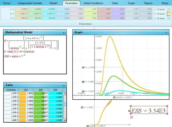
The starting step (see Figure 1) is to write in the Modellus Mathematical Model window the radiation power density function B (λ) which is given by
( ) ( )
where λ is the radiation wavelength, h is Planck’s constant, c is the speed of light, k is the Boltzmann constant and T is the temperature. The parameters h, c, k and T are defined in the Parameters ribbon (see Figure 1). The radiation wavelength is chosen to be the independent variable and the next step is to define in the Independent Variable ribbon the adequate domain interval for λ. This provides an opportunity for students to verify the range of values relevant for atmospheric radiation, in particular, the visible (solar) and infrared (terrestrial) radiation intervals. In the same ribbon students can also define the numerical step Δλ associated with λ. The following step is to represent B (λ) in graphical form using the Graph window. In figure 1 we show a Graph window with 3 different curves corresponding to 3 different temperature cases, T = 300 K, T = 400 K and T = 500 K. Figure 1 also shows the Table window where the values used to draw these curves can be explicitly displayed in table form.
Figure 1: Modellus blackbody radiation model showing in the Mathematical Model window Planck’s radiation power density function B (λ) and its numerical integration over the wavelength λ which leads to Stefan-Boltzmann law for the power radiated per unit area E. Also shown are the Graph window with 3 curves for 3 different temperatures, T = 500 K (orange), T = 400 K (green) and T = 300 K (cyan), the Table window and the Animation with a Pen object showing the graph of E as function of λ and a Variable ESB displaying Stefan-Boltzmann limit σT 4 for T = 500 K.
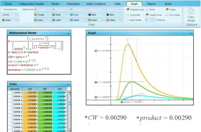
One of the advantages of using numerical solutions is to give introductory level students the opportunity to deduce Wien and Stefan-Boltzmann laws without having to perform the corresponding analytic derivations which are beyond the learning scope of most introductory courses. To deduce Wien displacement law students start by selecting one of the graphs representing B (λ) for a certain value of the
temperature T, for example, T = 400 K (see Figure 2). Selecting Tangent Lines in the Graph ribbon and using the mouse to move it along the graph, it is possible to visualize the tangent at every point along the curve and read in the abscissas axis the value of λ for which this tangent is horizontal. At this point λmax = 7.26×10⁻⁶ m, the
radiation power density attains its maximum value B (λmax) = 1.31×10⁸ W/m3.
Students can then compute the product λmaxT and verify that the numerical result is
approximately equal to the theoretical value of Wien’s constant, c W = 2.898×10⁻³ mK.
Students can interactively check that the fit between the computed and the theoretical Wien constant is improved when a smaller numerical step Δλ is used, and also that Wien’s law is similarly obtained using another B (λ) curve for a different value of T.
Figure 2: Modellus graphical deduction of Wien’s displacement law using a tangent line to the T = 400 K Planck density curve. To move the tangent line along the curve select and hold down the left mouse button or drag the Independent Variable button in the Animation Control bar. To select the curve maximum increase the number displaying precision selecting at least 5 decimal places in the Home ribbon. Then use the One step back or One step forward buttons and check the values in the Table window.
Finally, to deduce Stefan-Boltzmann law students use numerical integration to show that the power radiated per unit area E satisfies
∫ ( )
where σ = 5.67×10⁻⁸ W/(m2K4) is the Stefan-Boltzmann constant. The integration is programmed in the Mathematical Model window using the instruction (see Figure 1)
( )
with the initial condition E = 0. This is an application of the trapezoidal rule, a simple and useful numerical method for students just starting an introduction to scientific computation. The result of the integration can be visualized creating a Variable object ESB (see Figure 1) or plotting the graph of E as a function of λ. In figure 1 we show this graph as it is created by a Pen in the Animation area. The curve represents the accumulated area below B (λ) as λ runs through its domain and students can verify that it approaches a constant value approximately equal to the product σT 4.
4. Field actions discussion and conclusions
In this paper we have shown how Modellus can be used to develop interactive computational modelling activities that introduce mathematical physics models of interest in earth sciences contexts, to students with only basic secondary level knowledge of physics and mathematics and no prior knowledge of scientific computation. As an illustrative example, with insights on Modellus functionalities and potentialities for computer-assisted teaching and learning, we have described an activity about the blackbody radiation laws. This and other computational modelling activities have been field tested in introductory meteorology courses we have implemented for first cycle undergraduate university students at FCT/UAlg.
As shown by the average results of Likert scale questionnaires given at the end of each meteorology course (see Figure 3), the majority of students reacted very positively to the computational modelling activities. For example, defining the average opinion of a student as the average over all answers given by the student to the questionnaire statements, the results obtained for the 2011 edition of the introductory meteorology course showed that 95% of the students had a positive opinion, averaging 1 (30%), 2 (54%) or 3 (11%), 5% averaged no preferred opinion, and none of the students averaged a negative opinion. Students considered the activities useful for the learning processes in meteorology and for their professional training as a whole. In addition, Modellus was considered easy to learn, user-friendly and helpful for meaningful learning processes of mathematical physics models. The PDF documents used to present the activities were considered interesting and well designed. Students also considered favourably working in interactive engagement groups and using Modellus in other earth sciences subjects with appropriately adapted computational modelling activities.
On the other hand, content analysis of student coursework and evaluation tests has shown that the interactive computational modelling activities with Modellus and associated PDF documents were successful in identifying and resolving many student difficulties in aspects of physics, mathematics and scientific computation relevant for the meteorology course. In the 2011 edition the average grade was 70% and of the 53 students involved only 3 were not able to pass on the computational modelling component. The PDF documents proved to be very useful to explain the fundamental modelling ideas, problem solving processes and challenges to solve as well as to help students overcome more rapidly the initial difficulties of using Modellus. Students were able to create and explore the proposed mathematical physics models and simulations, establishing meaningful relations with the appropriate meteorological phenomena and operationally reifying many mathematical objects they previously considered worthless. To have real time visible correspondence between the animations with interactive objects, graphs, tables and
the mathematical model, with the opportunity to manipulate comparatively these different representations were again fundamental factors to achieve this. For example, the easy to draw Planck radiation curves helped students to better associate temperature with radiation emission and doing so by themselves constituted an extra motivation for learning. Student class performance and results on the activities also showed that introductory learning processes of mathematical physics models can involve differential equations solved by simple numerical methods and that students are able to appreciate the differences between numerical solutions and analytical solutions. The interactive engagement computational modelling activities with Modellus were thus successful in introducing mathematical physics models and scientific computation methods relevant for the earth sciences, helping students be better prepared for a posterior more advanced application of professional software systems or programming languages.
Figure 3: Introductory meteorology questionnaire and results for the 2011 course edition. For each questionnaire assertion the Likert scale starts at -3 and ends at +3, -3 stating complete disagreement, +3 complete agreement and 0 no preferred opinion. The bar graph shows the Likert scale distribution of the average student opinion per questionnaire assertion.
Future research will involve linking Modellus and other computer modelling systems, the development of new interactive digital documentation and software resources for earth sciences interactive engagement computational modelling activities, and new field research actions to test the new resources and analyse the corresponding learning and teaching processes.
5. Acknowledgments
We thank support by IDL, FCT/UAlg, UIED, FCT/UNL and Fundação para a Ciência e a Tecnologia, Ministério da Educação e Ciência (FCT/MEC), Programa Compromisso com a Ciência, Ciência 2007.
References
Bliss, J., & Ogborn, J. (1989). Tools for exploratory learning. Journal of Computer
Assisted Learning, 5, 37-50.
Blum, W., Galbraith, P., Henn, H.-W., & Niss, M. (Eds.) (2007). Modelling and
applications in mathematics education. New York: Springer.
Bork, A. (1967). Fortran for physics. Reading, MA: Addison-Wesley.
Chabay, R., & Sherwood, B. (2008). Computational physics in the introductory calculus-based course. American Journal of Physics, 76, 307-313.
Christian, W., & Esquembre, F. (2007). Modeling physics with Easy Java Simulations. The Physics Teacher, 45, 475-480.
diSessa, A. (2000). Changing minds: Computers, learning and literacy. Cambridge, MA: MIT Press.
Gould, H., Tobochnik, J., & Christian, W. (2007). An introduction to computer
simulation methods: Applications to physical systems. San Francisco, CA:
Addison-Wesley.
Halloun, I., & Hestenes, D. (1985a). The initial knowledge state of college physics students. American Journal of Physics, 53, 1043-1056.
Halloun, I., & Hestenes, D. (1985b). Common-sense concepts about motion.
American Journal of Physics, 53, 1056-1065.
Handelsman, J., Ebert-May, D., Beichner, R., Bruns, P., Chang, A., DeHaan, R., Gentile, J., Lauffer, S., Stewart, J., Tilghmen, S., & Wood, W. (2005). Education: Scientific teaching. Science, 304, 521-522.
Heck, A., Kadzierska, E., & Ellermeijer, T. (2009). Design and implementation of an integrated computer working environment. Journal of Computers in Mathematics
and Science Teaching, 28, 147-161.
Kortz, K., Smay, J., & Murray, D. (2008). Increasing student learning in introductory geoscience courses using Lecture Tutorials. Journal of Geoscience Education, 56, 280-290.
Libarkin, J., & Anderson, S. (2005). Assessment of Learning in Entry-Level Geoscience Courses: Results from the Geoscience Concept Inventory. Journal of
Geoscience Education, 53, 394-401.
McConnell, D., Steer, D., Owens, K., Borowski, W., Dick, J., Foos, A., Knott, J., Malone, M., McGrew, H., Van Horn, S., Greer, L., Heaney, P., 2006. Using Concept Tests to assess and improve student conceptual understanding in introductory geoscience courses. Journal of Geoscience Education, 54, 61-68. McDermott, L. (1991). Millikan lecture 1990: What we teach and what is learned
-closing the gap. American Journal of Physics, 59, 301-315.
McDermott, L., & Redish, E. (1999). Resource letter: Per-1: Physics education research. American Journal of Physics, 67, 755-767.
D. Meltzer, D., & Thornton, R. (2012). Resource Letter ALIP-1: Active-learning instruction in physics. American Journal of Physics, 80, 478-496.
Mintzes, J., Wandersee, J., & Novak, J. (2005). Teaching science for understanding:
A human constructivist view. Burlington, MA: Elsevier Academic Press.
Neves, R., Schwartz, J., Silva, J., Teodoro, V., & Vieira, P. (2012). Learning introductory physics with computational modelling and interactive environments. In A. Lindell, A.-L. Kähkönen, & J. Viiri (Eds.), Physics Alive: Proceedings of the
GIREP-EPEC 2011 Conference, (pp. 208-213). Jyväskylä: University of Jyväskylä.
Neves, R., Silva, J., & Teodoro, V. (2010). Computational modelling in science, technology, engineering and mathematics education. In Araújo, A., Fernandes, A., Azevedo, A., Rodrigues, J. (Eds.), Proceedings of the EIMI 2010 Conference:
Educational Interfaces between Mathematics and Industry (pp. 387-397). Bedford,
MA: Centro Internacional de Matemática and Comap Inc.
Neves, R., Silva, J., & Teodoro, V. (2011). Improving learning in science and mathematics with exploratory and interactive computational modelling. In G. Kaiser, W. Blum, R. Borromeo-Ferri, & G. Stillman (Eds.), International
perspectives on the teaching and learning of mathematical modelling: Vol. 1. ICTMA14 - Trends in teaching and learning of mathematical modelling (pp.
331-341). Dordrecht: Springer.
Neves, R., & Teodoro, V. (2010). Enhancing science and mathematics education with computational modelling. Journal of Mathematical Modelling and Application, 1, 2-15.
Ogborn, J. (1985). Dynamic modelling system. Harlow, Essex, UK: Longman.
Papert, S. (1980). Mindstorms: Children, computers and powerful ideas. New York: Basic Books.
Redish, E., Saul, J., & Steinberg, R. (1998). Student expectations in introductory physics. American Journal of Physics, 66, 212-224.
Redish, E., & Wilson, J. (1993). Student programming in the introductory physics course: MUPPET. American Journal of Physics, 61, 222-232.
Richmond, B. (2004). An introduction to systems thinking with Stella. Lebanon, NH: ISEE Systems, Inc.
Schwartz, J. (2007). Models, simulations, and exploratory environments: A tentative taxonomy. In R. Lesh, E. Hamilton, & J. Kaput (Eds.), Foundations for the future in
mathematics education (pp. 161-172). Mahwah, NJ: Lawrence Erlbaum
Associates.
Slooten, O., van den Berg, E., & Ellermeijer, T. (Eds.) (2006). Proceedings of the
GIREP 2006 conference: Modelling in physics and physics education. Amsterdam:
University of Amsterdam and European Physical Society.
Teodoro, V., & Neves, R. (2011). Mathematical modelling in science and mathematics education. Computer Physics Communications, 182, 8-10.
Teodoro, V., Schwartz, J., & Neves, R. (2012). Cognitive artifacts, technology, and physics learning. In N. M. Seel (Ed.), Encyclopedia of the Sciences of Learning (pp. 572-576). Dordrecht: Springer.
Wieman, C., Perkins, K., & Adams, W. (2008). Oersted medal lecture 2007: Interactive simulations for teaching physics: what works, what doesn’t and why.