TEM Journal 4(2):156-163
Transformation To Dual Physical Problems for
The Visualization of Abstract Topics
Suleyman Gokhun Tanyer
Department of Electrical – Electronics Engineering, Faculty of Engineering, Başkent University, Ankara, Turkey.
Abstract –Abstract topics are often very difficult to be visualized for the undergraduate students in mathematics, physics and engineering.Those problems could be represented by four fundamental examples; basic vector algebra, formation of standing waves, polarization of waves and optical filtering. In this work, the performance of teaching abstract topics using two different approaches are comparatively examined; the classical mathematical derivations and the transformation of abstract topics to visual dual physical problems. Efficiency of methodsare analysed statistically.Third year electrical engineering students’ exam results are examined using the empirical cumulative distribution function (ECDF). The transformation method is observed to be helpful, especially for below the average students. Formations of healthy normally distributed exam scores are observed.
Keywords – electromagnetics, empirical cumulative distribution function, optical filtering, performance measurement.
1. Introduction
Current undergraduate curriculum for mathematics, physics and engineering offer series of basic concepts for students. All these basics must be comprehended and be placed in the long term memories of each individual student to guarantee success in further education. More advanced lectures rely on the efficient utilization of those basics. Some problems are harder to be visualized than others due to the differences between their domains. The variance of the performance of a classroom increases due to the differences of each individual’s learning approach. Teaching abstract concepts requires understanding of the relationships of components of a set without the help of the basic senses of touching, seeing and hearing. This relationship of a set becomes even harder to be visualized in three dimensions when the process requiresrotations, projections and transpositions which could all be successively related. This is a common challengein teaching abstract topics to a classroom with a performance of high variance.
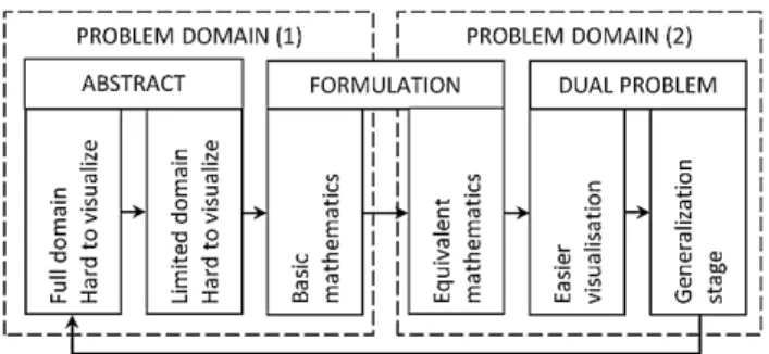
Fig. 1.Transformation of an abstract problem into a visual dual problem.
Some teachers are forced to aim the highest 70% of the classroom for success, leaving at least 30% just at the start. Some might think that this is fair enough, not to ‘waste the time’ of the majority. New programs are being developed to keep the whole classroom in contact; through interactions between classmates, utilizing visual simulation programs and supporting lectures with laboratories. Some examples
are: UC Berkeley’s webcast, Open Yale
Courses,MIT’s Open Courseware,Indian Institutes of Technology,and the Carnegie Mellon’s Open Learning Initiative [1–6]. Today, E-learningand mobile learning are educational research technologies of today [7–10].Those supporting materials are very helpful. Unfortunately, they can be used in “as is” format. Customizations are not possible due to their copyrights. It is not always possible to develop similar lecture materials due to the limitations oftime, effort and money. Visualizations are often ignored while teaching abstract topics due to the unavailability of practical solutions.Today, educational priorities and goals for curriculum development are being analyzedfor balancing the traditional and technological methods [11–13].
2. Transformation method for problem visualization
The problem of transforming an abstract problem into a visual one is not always an easy task. It is not possible to use the same practical solution for all problems. Thus, different approaches are necessary. A practical and systematic methodology is required.
In this work, a general procedure is proposed. It is summarized in five steps as shown in Fig. 1. First, the abstract problem domain is narrowed down to a single problem element. This allows easier handling of the abstract concept. In the second step, the problem is formulated using simpler mathematics. Third stage is the critical innovation stage where the instructor should be able to jump into a different domain using equivalent mathematics. If this is possible, simplified mathematics is used to introduce the new visual and hopefully more interestingproblem in the fourth step. Transformation of domains ishelpful since similar formulations are used. The instructor can spend more time on the formulation of a much easierproblem. This way leads to being understood by the whole classroom. Fourth step would be more successful if also supported by interactions between classmates. At the final stage, returning to the original problem requires much less concentration and background when compared to the original hard to handle abstract concept.When this transformation method is used several times, students are expected to follow more quickly and effectively.
3. Canonical Examples
Four canonical examples are selected in the field of fundamental electromagnetic wave theory; (1) basic vector decomposition using unit vectors, (2) formation of standing waves, (3) definitions of polarization, and (4) optical filtering using polarizing filters. The transformation method proposed herein is illustrated in the following examples.
a. Example 1 – Basic Vector Algebra
First example is the starting point invector algebra. It is widely selected by almost all universities around the world, since vectors are one of the most important basic tools in mathematics, physics and engineering. Vector algebra offers solutions in various fields in multidimensional problems including; statistical mathematics, control theory, electromagnetics, signal processing, power engineering, etc. Some drawings on the board are often found hard to be visualized by the undergraduate students, since often unskillfully drawn figuresare limited to two dimensions.
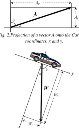
Fig. 2.Projection of a vector A onto the Cartesian coordinates, x and y.
Fig. 3. A car parked on a slope, its weight is the sum of parallel and perpendicular components with respect to the
road’s surface.
Drawing in perspective is not always possible. This is an important drawback in understanding of further topics.
Let us now analyze the problem of decomposition of a vector in space. Any vector A is equal to the sum of its projections defined by the three orthogonal unit vectors for some coordinate system. If Cartesiancoordinates are selected, vector A can be written as
�=����+����+���� (1)
whereux, uy, and uz are the unit vectors, and Ax, Ay,
and Az are the scalar projection values along the x, y
and z-axis[14, 15]. The projections can be found
using the dot product operator
��=�•�� =� cos(α) (2)
�� =�•�� =� cos(β) (3)
�� =�•�� =� cos(χ) (4)
whereα, β and χ are the directional cosines, A=|A| is the length of vector A. Now let us narrow our problem by assuming Ato be on the x-y plane defined by
TEM Journal 4(2):156-163
The graphical representation for (5) is given in Fig.2.Once the problem is simplified and formulated, it is now easier to transfer to a different problem domain. Students could easily examine forces acting on a car parked at a slope as shown in Fig. 3.The instructor could discuss the forward force component acting on the car. The visualization could be emphasized by examining the limiting cases; flat surface (α= 0)and the free fall (β= 0). Projections in three dimensions can be analyzed at the final generalization case.
b. Example 2 – Formation of Standing Waves
Propagation of a single electromagnetic (EM) wave is regarded as one of the hardest topics for an undergraduate student. Interactions of two EM waves propagating in opposite directions near a reflection point is far more complex to cope with. The dynamics are explained using mathematics, and sinusoidal waveforms are drawn for a stationary observer. EM waves travel at the speed of light, and must be slowed down. Further details force a dead end for visualizations. It is obvious that transfering to a different domain is necessary. Alternatively, thesound or water waves can be studied. They both have very similar dynamics; their propagation and standing wave mechanisms are almost equivalent. Sound wave alternative opens up whole new opportunities for the instructor. A guitar’s string, a flute or the harmonica which is frequently used in Baskent University.
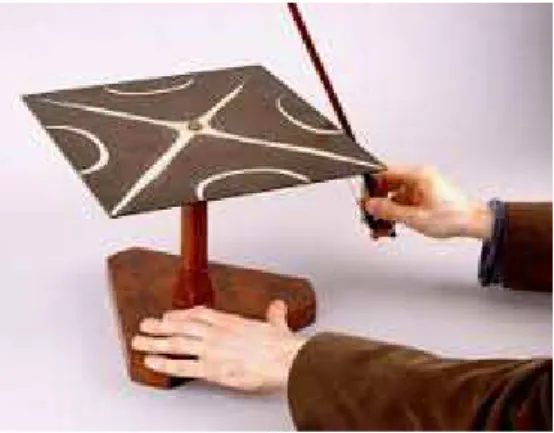
Simple demonstration tools can be developed; a stretched rope with one end tied to a wall, and the other is hold by hand. Up and down oscillationsapplied by the hand causes formation of standing waves in one dimension.Further, two dimensional standing wave formations can be observed by placing a50 ��x50 ��square metal plate on a comparable size speaker, or a simple excitation by a bow as illustrated in Fig. 4. For a list of similar examples visit [16–18].
If one sprinkles some amount of salt on the plate, salt particles are pushed towards the stationary nodes of the standing wave patterns, forming highly visual forms. It provides unforgettable experience for the students to observe various standing wave patterns forming instantaneously at different frequencies. Switching from the electromagnetic waves to sound waves enables students to develop very practical tools for visualizations. Musical instruments like; violin, guitar and drums are also good examples of standing wave generators. Numerous visualization solutions are possible.
Fig. 4.Formation of standing waves by the excitation of a metal plate by a bow.Note that, the salt crystals are
pushed to the stationary nodes [16].
c. Example 3 – Polarization of Transverse Electromagnetic (EM) Waves
Almost all textbooks introduce this topic by the list of possible polarizations; linear, circular and elliptical. Later, readers are informed by variations of circular and elliptical polarizations to be clockwise (CW) and counter clockwise (CCW) directions. They are forced to imagine looking towards the incoming wave to decide whether this rotation is CW or CCW. The mathematical derivations further complicates the problem. For a transverse EM wave propagating in an arbitrary direction defined by the spherical coordinates
�(�) = (�1�1cos(ω�+��+�2)
+�2�2cos(ω�+��+�2) (6)
wherer is the distance from the origin, �1 and �2 are the perpendicular unit vectors lying on the transverse plane[14]. Eq. (6) can be rewritten using phasors [19–25].
�(�,�) = (�1�1����+�2�2����)���•�. (7)
The rigorous analysis of the polarization using (6 and 7) is outside the scope of this work. Let us assumethat the wave propagation is along the +z-axis. Then, the electric field can be expressed as
�(�,�) =����cos(ω�+��+��)
+����cos�ω�+��+��� (8)
and similarly using the phasors,
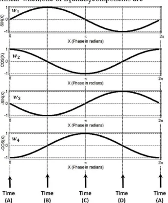
The polarization can be determined using the relative phase between the x and y components. Polarization islinear when;one of �xand�ycomponents are
Fig. 5. Sinusoidal waveforms �1, �2 and �3
representing phase values, (a) 0, (b) π/2, (c) -π/2 and (d) -1 respectively.
zero, or when they are in phase or out of phase by 180o.
∆�=��− ��=�π. (10)
Circular polarization is much harder to visualize. It is the case when �x=�y, and when
∆�=��− ��= (2�+ 1)π/2. (11)
It is defined to be clockwise and counter-clockwise when ∆θ= 900and −900, respectively. Elliptical polarization is the case when �x≠�y, and when
It is often very hard for the students to understand the physics behind the mathematics, especially when lecture lacks any visual support.
Polarization of an EM wave is defined by the motion of the tip of the electric wave vector, projected to the transverse field. This movement is a function of time and place, and the tip could travel with the speed of light in a helix trajectory. Unfortunately, the time and concentration allocated for this complex topic aregenerally very limited.
The polarization example can be analyzed by using a similar mathematical problem in mechanical engineering. Initially, the elliptical polarization can
(a)
(b)
Fig. 6. Motion of a mechanical piston at time instants A through D and back to A again (using the periodic waveform�1), shown in (a) one dimension, (b) two
dimensions.
be eliminated, and the phase of the phasor (∆θ) can be limited to four alternatives, and waveforms; �1
thru �4 are shown to oscillate out of phase according to Fig. 6. The phase differences are clear when they are evaluated at time instants; A, B, C and D. Now let us assume that each waveform represents the length of a mechanical piston as illustrated in Fig. 6 (a). The first piston’s motion is given in time (Fig. 6 (b)).
The piston modeling of the phase function is helpful for visualization the EM wave’s linear x-polarization. Linear y-polarization follows similarly. Combination of two pistons illustrated in Fig. 7 is much more visual when compared to the electric field formulated in (6–9). It is shown that at time instant (A) �1 = 0 along x-axis and �2= 1 as illustrated in Fig. 7 (a). Comparing also with Fig. 5, it is now obvious that �1 will increase from 0 to 1 while �2 will decrease from 1 to 0 along the circular
path to reach the point (B). This visualization is expected to be clear for 100% of the classroom to beclockwise. It should also be clear that polarization becomes counter-clockwise if �4 is used instead of
TEM Journal 4(2):156-163
�2 for the y-axis as shown in Fig. 7 (b). Eqns. (6-12)
state the same mechanism using mathematics.
(a)
(b)
Fig. 7.Motion of two mechanical pistons pushing in x and y axis, using waveforms �1 and �2 respectively, (a)
clockwise rotation, (b) counter-clockwise rotation.
d. Example 4 – Optical Filtering Using Polarizers
Polarizing filters are analyzed both in undergraduate and graduate level optics courses. A common example is studied here.
A total transverse EM wave propagating along the z-axis can be written as the sum of the two linearly polarized waves as given in (13).
���(�) =��(�) +��(�) (13) where
��(�) =�����−��� (14)
��(�) =�����−��� (15)
Let us place two polarizing filters in front of the propagating wave ��� as shown in Fig. 8 (a). The optical transfer functionsfor the polarizing filters are illustrated in Fig. 9.It is almost obvious that the output of Fig. 8 (a) is zero. First filter stops the x-polarized component given in (14) and the remaining y-polarized wave of (15) is stopped by the second filter. Students use this clear information to falsely deduce that it is also true for the case shown in Fig. 8
(b). Even rigorious derivationsare observed not to convince even top students in the class.
(a)
(b)
Fig. 8. Multiple stage optical filtering, ��� is the input and (a) two filtering stages, �� is the x-polarized and �� is the y-polarized filters, (b) similar to (a) but a third diagonally
polarized filter �� is placed in between the two filters.
Fig. 9.Three optical polarizing filters drawn on the transverse plane.
This example is a good validation of the visualization problem analyzed in this work. It is really hard to convince students that the output could be different from zero due to the presence of Fx and Fy. It seems almost true that; the x and y
polarized components of ��� are stopped by �x and
�y, and this must yield a zero output. The function of
the second optical filter,��, isnot very clear and is the source of this confusion. The related vector analysis is summarized in Fig. 10 (a). The input field ��� can be decomposed into x and y polarized waves (Fig. 2). �� stops the x-polarized component of ��� as illustrated in Fig. 10. (b) so that, the input to the filter�� is only the y-polarized �1. It is interesting to
observe that the output of ��, �2, does have an
x-polarized component. This is the missing link that even if �x stops all of the x-polarized wave initially, �d rotates its output so that x-polarization reappears.
fail to answer this exam question. This is possibly because complex mathematicalinformation
(a)
(b)
Fig. 10. Three stage optical filtering using ��, �� and ��, (a) simple two dimensional drawing, (b) summary of
vector projections of ��� through ����.
(a)
(b)
Fig.11. Sail boats moving with the force of wind, (a) two sail boats moving towards the wind flow (photograph),
http://news.mulletboatracing.co.nz/ (b) wind force components on sail boats for different angles (boats in
gray directions cannot profit from the wind).
is stored in the short-time memory if not supported visually.
It is necessary to move on to another domain to examine what is really going on. Following the steps
proposed in Fig. 1, the problem can be simplified and moved into a more visual domain that has equivalent
(a) (b)
Fig.12. Sail boats moving with the force of wind, (a) sail transfers wind forces component as �1, (b) the keel of the
boat projects sail’s force to the boat rudder.
Fig.13. The place and shape of the keel of the boat, http://en.wikipedia.org/wiki/Keel
mathematics as summarized in Fig. 10 (a). The new domain should illustrate the unpredictable nonzero outcome physically. For this example, the physics of sailing is examined. Sails travel towards the wind direction with the power of wind itself as shown in Fig. 11. Please notice the wind direction is aligned with the flags on the bridge. Both boats travel almost towards the wind, and it would not be wrong to say that it is unbelievable. Projections of wind power can be analyzed in three steps similar to the original problem. First, wind force is partially transferred to the boat by the sail as illustrated in Fig. 12 (a). Then, this force is projected once again as a forward force by the keel of the boat Fig. 12 (b). The keel is a long plate underneath the boat’s body as shown in Fig. 13. It is interesting that the wind force �1, and its projected force �out clearly have opposing vectoral force components along the axis of the boat.
4. Statistical Analysis of Exam Results
TEM Journal 4(2):156-163
often not very helpful. Statistical methods valid for finite setof observations should be used since the
(a)
(b)
Fig.14. (a) The CDF and its first and second derivatives for the standard normal distribution, (b) the ECDF and its first and second derivatives for 100 observed samples of
(a), 50 independent sets are used.
number of students could be as small as 10. In this work, the exam scores are examined using the empirical cumulative distribution function (ECDF) [26–28].
For an ordered set of N elements, Xn=
{xn: xn∈ℜ, n=1, 2, , N}where xp<xr for 1 ≤ p
<r ≤ N, the ECDF is defined as
���,�(�)
= � 0 �/�
1
�<�1 ��≤�≤��
��≤�
(1≤�≤� −1) (16)
wherethe ECDF, ���,�, converges to the CDF, �� for N →∞. Note also that the probability density function (pdf) and the CDF is related by
����{�<��} =��(��) = � ��(�) ��
−∞ �� (17)
��(��) =���� ��(�)��=�
�
. (18)
(a)
(b)
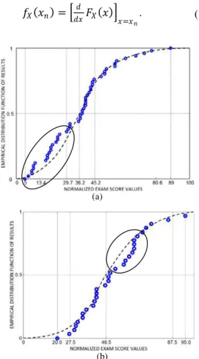
Fig. 15. The ECDF results for the EEM-323 for semesters; (a) Fall 2013, (b) Fall 2014.
The CDF and the pdf are the asymptotical functions valid only when N→∞. For a finite set of exam results, pdf can be estimated numerically. Least squares estimation for the pdf can be used as shown in Fig 14. Note that, the first derivative of the least squared estimation of ECDF (LSE-ECDF) is the least squared estimate of the empirical pdf (LSE–epdf). One further derivative of LSE–epdf illustrated in Fig. 14 (b) shows that the score domain can be divided into two regions where the zero crossing (middle) point is the observed value for the mean.
For small number of observations (exam scores), assumption of any type of distribution, including normal distribution is not accurate. Thus, mean and standard deviation values are not accurate. However, the EPDF and its derivatives provide statistical information for any type of observed distribution even for a classroom of just ten students. Note also that, it is possible to compare the EPDF results even if the number of students are not equal.
5. Numerical Results
Electromagnetic Wave Theory II (Fall2013 and Fall 2014 semesters). Both set of exams are developed to be equivalent. In the first year, conventional teaching method is used. In the following year, fundamental topics are taught using the transformation to visual dual problem domain analyzed in this work. The canonical questions given in Sect. 3 are used in preparing of the quizzes, midterm and final exams.Individual scores for those preselected questions are added to form a single reference test score. It is then normalized to 100 for each student. Those combined scores are statistically analyzed. The ECDF results are given in Fig. 15. Note that the students below the average form a statistically lagging group (shown inside the ellipse) as illustrated in Fig. 15 (a). On the following year, it is observed that visual transformation of the abstract topics helps those students to catch up with the rest of the class. It is interesting to observe that similar improvement is observed for the above the average students as shown inside the ellipse (Fig. 15 (b)).
6. Conclusion
It is observed that classical method of teaching could divide the classroom into two groups with different mean and standard deviation values. On the other hand, visualization of abstract topics helpsthe classroom’s observed scoresto form a population with the same distribution. The visualization method is found helpful to students, especially the below average students. They are observed to catch up with the rest of the class, forming a population of the same distribution.
References
[1]. Cihan P., Kalıpsız O., “Evaluation of students’
skills in software project,” TEM Journal, vol. 3, no. 1, 2014.
[2]. Webcast, University of California, Berkeley,
http://webcast.berkeley.edu/
[3]. Open Yale Courses, http://oyc.yale.edu/courses
[4]. Open Courseware, Massachusetts Institute of
Technology, http://ocw.mit.edu/index.htm
[5]. NPTel Channel List, Indian Institutes of
Technology http://www.youtube.com/user/nptelhrd
[6]. Open Learning Initiative, Carnegie Mellon
University, http://oli.cmu.edu/
[7]. Özyurt Ö., Baki A., Güven B., Karal H., “A fully
personalized adaptive and intelligent educational hypermedia system for individual mathematics teaching-learning,” TEM Journal, vol. 1, no. 4, 2012.
[8]. Kou H., Wan Z., “Research on E-learning-based
educational technology training model for college teachers,” Hybrid Intelligent Systems, HIS '09. Ninth International Conference on , vol. 3, 2009.
[9]. Saracevic M., Kozic M., Selimovic F., Fetaji B.,
“Improving university teaching using application
for mobile devices based on Netbiscuit platform and integration with the LMS,” TEM Journal, vol. 2, no. 1, 2013.
[10]. Ebibi M., Fetaji B., Fetaji M., “Combining and
supporting expert based learning and academic based learning in development mobile learning knowledge management system,” TEM Journal, vol. 1, no. 1, 2012.
[11]. Garrett J., Coleman, D. S., Austin L., Wells J.,
“Educational Research Priorities in Engineering,” 38th ASEE/IEEE Frontiers in Education Conference, 2008.
[12]. Hira R., “Undergraduate engineering education
curriculum and educational research,” IEEE International Symposium on Technology and Society, 1996.
[13]. Vasileva M. Bakeva V., Vasileva-Stojanovska T.,
Malinovski T., Trajkovik V., “Grandma’s games project: Bridging tradition and technology mediated education,” TEM Journal, vol. 3, no. 1, 2013.
[14]. Cheng D. K., Fundamentals of Engineering
Electromagnetics, Prentice Hall, 1992.
[15]. Halliday D., Resnick R., Krane K. S., Physics, Fifth
Ed., John Wiley & Sons Inc., New York, 2002.
[16]. A list of related links, Web portal for Physics 102,
Özcan E., Instructor in Physics, Boğaziçi
University,
Turkey,www.phys.boun.edu.tr/~ozcan/lectures-/phys102spring12/Phys102Spring12/links.html
[17]. The top five collections of free university courses:
http://www.openculture.com/2008/09/the_top_five_ open_course_collections.html
[18]. Top 10 Universities with free courses online:
http://www.jimmyr.com/blog/1_Top_10_Universiti es_With_Free_Courses_Online.php
[19]. Hecht E., Optics, 2nd Ed, Addison Wesley, 1987.
[20]. Guenther R., Modern Optics, Wiley 1990.
[21]. Waynant R. W., Ediger M. N., Editors,
Electro-Optics Handbook, Optical and Electro-Optical Engineering Series, McGraw-Hill, 1994.
[22]. Moller K. D., Optics, University Science Books,
1988.
[23]. Pedrotti F. L., PedrottiLS, Introduction to Optics,
Prentice-Hall, 1987.
[24]. Waynant R.,Ediger M., Electro-optics Handbook,
McGraw-Hill, 1994.
[25]. Born M., Wolf E., Principles of Optics, Pergamon
Press, Oxford, 1975.
[26]. Gentle J. E., Computational Statistics, Springer
Dordrecht Heidelberg, pp. 344–350, 2009.
[27]. Tanyer S. G., “Generation of quasi-random
numbers with exact statistics,” 22. Signal Process. Communicat. Applicat. Conf. (SIU), pp. 281–284, 2014.
[28]. Tanyer S. G., “True random number generation of
very high goodness-of-fit and randomness qualities,” 2014 Int. Conf. Math. Comput. in Sci.
and Industry, (Invited), Sept. 13–15, pp. 213-215,
2014.
Corresponding author: Gokhun Tanyer