HOW THE MAJOR CAPITAL MARKETS INTERACT IN THE
WORLD: A VAR APPROACH
António Pedro Cardoso Costa
Dissertation submitted as partial requirement for the Master’s
degree in Finance
Orientador(a):
Prof. Doutor José Dias Curto, Prof. Auxiliar, ISCTE Business School, Quantitative Methods Department
i
Abstract
For many years, financial data analysis, such as stock prices and returns, has been receiving a lot of attention from researchers. A variety of methods has been proposed and implemented in order to forecast these variables and also to study the relation and interaction between them.
The main goal of this thesis is to analyze the interaction between the following seven indexes the PSI20 (Portugal), CAC40 (France), IBEX35 (Spain), NIKKEI225 (Japan), DAX (Germany), NASDAQ (United States of America), and FOOTSIE100 (United Kingdom).
The analysis was based on a database with daily observations between 2000 and 2010, and the econometric methodology includes: Augmented Dickey-Fuller, KPSS, Granger causality test and VAR models.
Keywords: VAR models, Granger causality, Capital Markets, Returns
JEL Classification: G10 – General Financial Markets, C10 – Econometric and
ii
Resumo
Durante as últimas décadas, a análise de dados financeiros, tais como, os preços das acções e os seus respectivos retornos, tem sido alvo de muito estudo por parte dos investigadores. Existe uma variedade de métodos que têm sido propostos e implementados com o objectivo de prever essas variáveis e também de estudar as relações interacções que têm entre si.
Esta tese tem como principal objectivo analisar a interacção entre os seguintes sete índices: o PSI20 (Portugal), CAC40 (França), IBEX35 (Espanha), Nikkei225 (Japão), DAX (Alemanha), NASDAQ (Estados Unidos da América), e FOOTSIE100 (Reino Unido).
A análise efectuada teve como suporte uma base de dados com observações diárias entre os anos 2000 e 2010, e a metodologia econométrica incluí os testes: Augmented Dickey-Fuller, KPSS, causalidade de Granger e os modelos VAR.
Keywords: Modelos VAR, Causalidade de Granger, Mercados de Capitais, Acções
JEL Classification: G10 – General Financial Markets, C10 – Econometric and
iii
Agradecimentos
Ao meu orientador Professor Doutor José Dias Curto por todas as críticas construtivas, comentários, sugestões e disponibilidade que contribuíram para melhorar o input final.
A toda a minha família por todo o apoio, e força que me deram.
A todos os meus amigos que sempre me incentivaram a não desistir e a concluir esta tese.
E finalmente à Teresa por toda a paciência, e compreensão que evidenciou ao longo deste últimos tempos.
iv
Index
1 - Introduction ... 1
2 - Literature Review ... 4
3 - Methodology ... 9
3.1.1 - Augmented Dickey-Fuller test ... 10
3.1.2 - KPSS test ... 11
3.3 - Granger Causality ... 13
3.4 - Information Criterion ... 15
3.4.1 - Akaike Information Criterion ... 15
3.4.2 - Schwarz Criterion ... 15
3.5 - VAR methodology ... 16
4 - Econometric Methodology and Data Analysis... 18
4.1 - Data ... 18
4.2 - Econometric Methodology ... 19
4.3 - Granger causality test ... 23
4.4 - VAR Models ... 26
5 - Conclusions ... 33
References ... 35
Appendix ... 37
Appendix 1 - VAR equations obtained from the estimated output ... 38
v
Tables Index
Table 1 - ADF test results for Adj. closing prices ... 19
Table 2 - KPSS test results for Adj. closing prices ... 20
Table 3 - ADF test results for returns ... 21
Table 4 - KPSS test results for returns ... 21
Table 5 - Granger causality test for returns ... 23
Table 6 - Granger causality test for returns (conclusion) ... 25
Table 7 - Results of VAR for returns ... 27
Table 8 - Interpretation of VAR equation for CAC_RET ... 30
1
1 - Introduction
For many years, financial data analysis, such as stock prices and returns, has been receiving a lot of attention from researchers. They continue to make efforts in order to find more accurate ways to study and predict their behavior. A variety of methods has been proposed and implemented in order to forecast these variables and also to study their relation and interaction.
Usually, investors hold portfolios comprising more than one financial instrument, being of great importance to analyze each component of the portfolio and their relations. Thus, in practical terms, multivariate analysis of financial data might be more appropriate than univariate analysis.
To conduct our research we selected seven stocks indeces that are representative or developed capital markets in the world, thus, our selection is: the PSI20 (Portugal), CAC40 (France), IBEX35 (Spain), NIKKEI225 (Japan), DAX (Germany), NASDAQ (United States of America), and FOOTSIE100 (United Kingdom). Since, we decided to work with daily observations our data ranges from 2000 to 2010.
In the recent past years the Capital Market have been unstable and volatile.
In the last decade we had some financial crisis all over the world, but the subprime crisis was the one that affected all the markets on a worldwide scale. The terrorist attacks on September 11 in United States of America was the first occurence that led us to the subprime crisis, i.e., in order to minimize the effects of September 11 in the markets, the United States, started to lower its interest rates, and the banks made some high-risk loans even to people that do not have reliable goods or earnings to pay their loans. The banks and management funds, in order to earn more money, started to buy subprime titles, and then sold them to other companies. However when the interest rates raised and the real state market decreased people started to fail their loans payments, therefore some credit institutions, such as Lehman Brothers fell into bankrupt. With this
2 lack of liquidity the consumption fell and the industries had less earnings. The subprime conduct us to a deep and serious global crisis that snapeed in 2008.
On the next two semesters (the first of 2008 and the first of 2009) there was a large fall in GDP (Gross Domestic Product) not only in U.S. but also in Europe, and the global banking and financial system was on the verge of collapse.
With the intervention of the IMF – International Monetary Fund ( an organization that is controlled by the United States of America) the continuity of Euro currency was ensured, and with this intervention was also defined the aid financial packages to some European countries.
The financial aid packages to banks and financial markets launched by the governments of imperialist countries and also by some others countries like China and Brazil are an important moment in this global crisis. The imperialist states, which had previously driven the speculative process, had now a role of "insurance companies" in the financial sector, with debenture loans to directly inject liquidity into banks, or committing themselves to external entities through these financial aid packages. Thus, the governments managed to save banks and prevent a general collapse of the global financial system. On the other hand, these packages could also curb the dynamics of "free fall" of world economy, starting a fragile recovery in the second half of 2009.
But the great indebtedness of the states began to reach weaker countries like Greece and Portugal, because of this situation these countries cannot sustain the debt contracted, bringing two alternatives, i.e., or the countries begin to fail their payments, or they are nearly approaching that situation. Despite being small, these countries are part of one of the main world poles, the European Union. Thus, its economic and political situation has contagion effects in all Europe and also in the world economy. By lowering their ratings and classifying them as "junk", the U.S. rating agencies contributed to the increase of the refinance interest rates of public debt of these countries, and consequently to a devaluation of the euro against the dollar.
At this stage of the global crisis, the contagion effects have impact on a worldwide scale, since the banks in the United States banks have invested several billions of dollars in public debt of some important European countries (Germany, France, Spain, etc. ...).
3 Due to the interdependence on capital markets worldwide, the main purpose of this thesis is to prove how the stock markets interact among themselves. In order to evaluate and test that interaction we use the VAR methodology.
Through the VAR methodology we can conclude that the returns from the day before on the American index NASDAQ have impact in the current returns of all the indeces analyzed including NASDAQ itself. The German index DAX follows the same pattern with only one exception, the returns of the day before from DAX do not have impact on the present returns of DAX. In the opposite way we have NIKKEI225 and PSI20, the returns of these two markets are only influenced by returns of the day before from FOOTSIE100 and PSI20 itself, in the case of PSI20, and NIKKEI225 is influenced by NASDAQ and NIKKEI225 itself.
Regarding the structure of this thesis it is composed by 5 chapters, among which is included the introduction. On the next chapter we present a brief literature review enframing this theme in a theoretical way. On chapter 3 we briefly describe the tests that we will use such as: Augmented Dickey-Fuller Test, Pairwise Granger Causality, and Vector Auto regression (VAR) models. The empirical results of our work and their respective analysis will be presented on chapter 4. Finally, the last chapter will be dedicated to highlight the main conclusions of our research, and also to provide some guidelines for future researches on this theme.
4
2 - Literature Review
Due to a great popularity of VAR methodology, there are several studies that address its issue, relating different variables such as: macroeconomic variables (GDP, inflation, etc ...), capital market components (price, returns, etc ...), and commodities (oil, etc ...).
The papers referred below, point different relationships between variables with different periods of time. All use VAR models to describe the linear relationship between the variables under study and they are summarized in a chronological sequence.
Edwards (1998) used VAR methodology and the Granger causality test to study the behavior of interests rates Mexico, Argentina and Chile. The author selected a database with weekly and monthly observations between 1992 and mid 1998. Through the econometric methods applied, Edwards concluded that when the financial crisis burst contagion effects were significant.
Nagayasu (2000), had as main purpose to study the Asian financial crisis, using a database with daily observations related to capital markets and rates of change of the countries Thailand and Philippines for a period between 1996 and 1998. For this analysis the author used the following statistical and econometric tools: Unit root test, Granger causality test, VAR methodology and cointegration. Through this research Nagayasu (2000) observed that the price movement of some sectors of Thailand’s stock markets (particularly in banking and financial) was causing the statistical variations of Philippine currency. It can also be concluded that the correlation between some of the variables is stronger during the crisis period, which confirms the importance of interlinkages between financial markets.
Another relevant study that employed the VAR methodology was carried out by Bazdresch and Werner (2000). These authors sought to examine the relationship of contagion that Mexico suffered from the crises in Russia, Brazil and Asia in the period between 1997 and 1999. Bazdresch and Werner (2000) resorted to the VAR methodology in order to study these relationships and the findings suggested that the
5 crisis spreading to Mexico increased along the years with special emphasis when the Russian crisis intensified. Despite having suffered with this financial crisis it is important to refer that the United States economy had a positive effect in Mexico reducing the impact of the crisis.
Caiado (2002), used VAR models in his study with the aim of describing the relationship between interest rates and the inflation rate in Portugal, and also if the inflation rate has an impact in determining the future value of interest rates.
As a conclusion of this work the author refers, the existence of a non-reciprocal causal relationship between inflation and interest rates, which is decreasing after a total price liberalization of lending operations and deposit-taking. Throughout this study it is also possible to measure that bivariate VAR models are better to predict interest rates in the short term, compared with the univariate autoregressive models. Conversely the univariate models are more effective when include long-term values of interest rates as regressors.
Yang et al. (2004), applied both the Granger causality test and the VAR methodology to daily data for the stock markets of several Asian countries between the years 1990 and 2000. The aim was to test the evidence of contagion between stock markets (Hong Kong, Indonesia, Korea, Malaysia, Thailand, Philippines, Singapore, Taiwan, and Japan), as well as to explore the importance of interactions between stock markets and transmission channels during the crisis. The results pointed for the widespread existence of contagion effects following the Asian crisis of 1997.
In order to study the impact of the economic growth rate in Brazil, and taking into account the fiscal policy and technological changes, Dias and Assis (2005), chose a database with annual observations between the years 1951 and 2000. The authors concluded that during the period under review the economic growth was being driven by the increase of the two variables under study, According to these authors the greater the public investment and technological development are, the higher will be the economic growth rate.
Shachmurove (2005), tried to explain how a shock in the markets of the Middle East affects the other markets of this region. This work also analyzes the interdependence
6 between the returns on the capital markets Egypt, Israel, Jordan, Lebanon, Morocco, Oman, and Turkey.
The database used in this paper contains daily observations, and used the VAR methodology. Throughout this study it was concluded that none of the analyzed markets is totally independent, even though the interrelationships are not so large. Following this two further conclusions were obtained: first due to this small interdependence foreign investors benefit from this situation by including stocks of these countries in their portfolios. Second, these countries will take profit if their capital markets are more accessible to foreign investors, adapting them to international law in order to protect foreign investors.
Cheong et al. (2006), investigated possible interrelations between exchange rate uncertainty, international trade and competitiveness in trading prices, based on data from the UK. With the obtained results it was possible to conclude that a negative variation in the exchange rate’s volatility adversely affected the volume of exchanges. It was also possible to infer that a possible integration of the Euro in the UK would have a positive impact on the variables analyzed.
Lin et al (2008), examined the linkages between the expected growth rate implied by the prices of index futures and the rate of return of the underlying spot index market in Japan, United States of America and Taiwan, in order to perform the research the authors used VAR methodology and the Granger causality test. The main conclusions of the research were that these relationships are more evident in the Taiwanese market than in the Japanese and American market, and that this happens due to market imperfections, in this way, the greater the market imperfections are, higher the relationship between these two variables is.
Since the purpose of this study was to analyze the relationship between real estate investment funds, the stock market, and real economic activity in the United States of America, Laopodis (2009), VAR methodology was used to conduct this study using a database that ranges from 1971 to 2007. As main conclusions of this investigation, it was noted that the variables Equity and Mortgage have similar relationships with the stock market and industrial production, and also that REIT (Real Estate Investment Trusts) categories are more related with a sub index defined in the study than the market
7 share in general. However it was found that there are relations in short term between the variables since 1970.
Due to the existence of few studies regarding oil, Guidi (2010), employing the VAR methodology, examined the relationship between oil prices and the UK's manufacturing and services sectors performances, taking into account some macroeconomic variables, such as, product manufacturing (IPM), index production services (IPS), real wages manufacturing (RWM), real wages services (RWS), real effective exchange rate (REER), long-term interest rates (LR), short-term interest rates, and real oil prices (ROP).
Based on this research it was possible to conclude through linear specification that the variation of oil price affects more the manufacturing sector in a positive than in a negative way. The author also concluded that in a short period, wages are affected adversely.
Zeaiter (2010) conducted another study related with oil. The aim of this study was to examine the impact of the increase in the imported oil price on the U.S. Economic Activities prior to the 2007-08 oil crises. The author used quarterly data from 1948 to 2000, and he concluded that the net increase in the imported oil price had more influence in determined economic activities than in the rising price of oil produced domestically. It can also be concluded that both prices show similar significant effects on unemployment and output growth.
Since the main goal of this paper is to analyze the situation of Nigeria, Ndaka (2010) studied the long-term relationships between financial development and economic growth in Nigeria. For this study it was used a database with annual periodicity that ranges from 1960 to 2005. Through bi-directional causality was possible to conclude that a weak relationship between economic growth and financial development happens in Nigeria. Thus the author suggested that it would be necessary to produce sector reforms, and the authorities should have policies needed to reverse this trend.
As the sections attest, the VAR methodology and the granger causality test have been extensively applied. They have been employed to a multiplicity of countries and sectors, and have taken in consideration a very difference range of years and variables. The
8 results have, nevertheless, always been both enlightening and trustworthy, which has contributed to classify these procedures as reliably adjustable. These are the reasons why they were chosen as the methodologies the current study resorted to, and will be described throughout the next section.
9
3 - Methodology
The main goal of this chapter is to give a brief description of the statistical procedures and the tests used in our analysis. So, first we discuss the definition of stationarity that is included in the description of unit root tests, Augmented Dickey-Fuller, and KPSS, and then we present a brief description of the tests used in our analysis, Granger Causality, the Akaike Information Criterion, Schwarz Criterion and the Vector Auto regression (VAR) models.
In this work we deal with returns instead of prices, because returns are in general stationary. If we wanted to work directly with prices, we could use the cointegration technique. However, if we use directly prices without cointegration in our research we could incur in the spurious regression issue. The spurious regression is a phenomenon that happens when we try to do a regression of a stationary series in another non-stationary series. This type of regression is a meaningless regression, in which we observe a statistical relationship that does not exist in long term. For example the migration of storks and the birth of babies, by chance, these two variables can show a strong relation, but in reality these two variables do not have any kind of relation.
This chapter is based on the books: of Tsay (2005), Marques (1998), and on the paper of Caiado (2001).
10
3.1 - Unit root tests
3.1.1 - Augmented Dickey-Fuller test
The main objective of the Augmented Dickey-Fuller is to test the existence of a unit root or not. Both tests (Dickey-Fuller and the Augmented Dickey-Fuller) follow the same pattern, however in practice the Dickey-Fuller is not very useful to test the existence of unit roots because this test assumes that the residual variable is not autocorrelated, i.e, follows a random walk under the null hypothesis or an AR(1) under the alternative hypothesis. There are very few series that can be described by these simple processes. We know that in the regression
(1)
with , if is autocorrelated, then the OLS estimator ̂ is inconsistent. In a situation like that Dickey Fuller tests are not valid. In order to pass this situation Dickey and Fuller (1979) developed a test for a more general case where follows an auto regressive process of order p, AR (p)
∑
By the reparametrization of the model, the ADF can be presented as follows
∑
With this formula we can now perform the Augmented Dickey-Fuller test based on the following hypothesis:
11 {
If we don’t reject , we can say that exists at least one unit root, thus the variable under analysis is non-stationary. On the other hand if we reject we conclude that the series is stationary, i.e., there is no unit root.
As a side note, it should be mentioned that, stationary series can be evaluated in two different ways. Strict stationarity and weak stationarity, (in order to have a series that has strong stationarity all the variables must have the same distribution from 1 to , i.e., , generally this is very uncommon to observe, in order to have a series with weak stationary three conditions must be observed (constant mean and variance, and covariance) these conditions only take in account the first two moments of the probability distribution , due to that the series must have moments until the second order (mean, variance, and covariance). A series with weak stationarity has constant mean and variance.)
3.1.2 - KPSS test
The KPSS test was proposed by, Kwiatkowski, Phillips, Schmidt and Shin (1992). The main difference between KPSS and the other unit root test is that in the other tests the series is assumed to be (trend -) stationary under the null hypothesis. The KPSS statistic is based on the residuals from OLS regression on the exogenous variables
:
The LM statistic is defined as:
12 Where is an estimator of the residual at frequency zero and where is cumulative residual function:
∑ (7)
based on the residuals where We point out that the estimator used in this calculation is different from the one used by GLS since it is based on a regression involving the original data.
The KPSS test has the two following hypothesis:
{
If we reject , we can say that, the series is non-stationary, on the other hand if we don’t reject we conclude that the variable is stationary.
13
3.3 - Granger Causality
The Granger Causality concept was created by Granger (1969). This type of causality is often tested in the context of VAR models, and it contributed to Granger’s popularity. The basic idea of Granger causality states that X Granger causes Y, i.e., the past values of X contribute to improve the forecasts of the present value of Y, assuming everything else is constant.
The Granger causality tests show us the existence of causal relations in a purely statistical sense.
In order to proceed with the Granger causality test we have to respect the following steps:
1) Estimate the best auto-regressive model for ; 2) Add the lags that we want in the equation , i.e.,
3) We have to test the joint significance of the estimate for the parameters
;
4) In order to test the Granger causality stated in Section 2, we compute an F test with the following hypotheses:
{
Through the probability associated to the F test:
⁄ ⁄ ⁄ ⁄ (11)
14 we can conclude whether or not to reject , If we reject we conclude that X causes Y, if we don’t reject , we say that X does not cause Y.
Due to the interaction effect we can have an unilateral effect (example: X causes Y, and Y does not cause X), or a bilateral effect (example: X causes Y, and Y causes X).
15
3.4 - Information Criterion
3.4.1 - Akaike Information Criterion
The Akaike Information criterion is directly generalized to the multivariate case, and in the context of the VAR models is given by the following equation
|∑ |
(12)
The Akaike Information Criterion is a tool to select the best model, and we chose the largest lag that minimizes the AIC value.
3.4.2 - Schwarz Criterion
Schwarz has developed a criterion that is given by the following expression
|∑ |
(13)
The Schwarz Criterion like the AIC is also a tool to select the best model, and we must choose the lag that minimizes the SC value.
16
3.5 - VAR methodology
The vector autoregressions (VAR) models emerged in the 80’s by Sims. Since the VAR approach treat all variables symmetrically without imposing any restriction in the dependence and dependence between them, VAR methodology allows to describe each one of the endogenous variables in the system as a function of lagged values of all endogenous variables.
The main objective of VAR is to examine linear relationships between each variable and its lag values, all the other variables, and their lagged values.
This methodology examines the existence of interdependence relations between the variables and allows us to evaluate the dynamic impact of random disturbances on the variables of the system.
In VAR models, the number of lags is usually chosen based on statistical criterion such as Akaike or Schwarz.
The expression of VAR (p) is given by:
Where is a vector of endogenous variables, is a vector of exogenous variables, and are matrices of coefficients to be estimated, and is a vector of innovations that may be contemporaneously correlated but are uncorrelated with their own lagged values and uncorrelated with all of the right-hand side variables.
Only in the second members of VAR equations appear lags values of endogenous variables. The application of applying the ordinary least squares method (OLS) will produce consistent estimates in the estimation of each system equation, even if the errors are correlated.
17 So we will use all the method described above (the Augmented Dickey-Fuller, the KPSS, the Akaike information criterion, the Scharwz criterion, the Granger causality test, and the VAR methodology). The following section will focus not so much in the methods employed, but rather oh how the data were collected and then analyzed.
18
4 - Econometric Methodology and Data Analysis
4.1 - Data
The main goal of this dissertation is to observe how some of the Capital Markets in the world interact among them. The criterion used to choose the indices was based on the importance that the country to which the index belongs has to the world economy. Thus our data base is composed by the adjusted closing prices of seven indexes: PSI20 (Portugal), CAC40 (France), DAX (Germany), FOOTSIE100 (United Kingdom), IBEX35 (Spain), NIKKEI225 (Japan), and NASDAQ (United States). To perform our analysis we used a database with daily frequency that ranges from January 2000 to December 2010. Our database information was obtained via Yahoo Finance, except in the case of PSI20. In this case we obtained our data via Bloomberg, because Yahoo Finance only had daily adjusted closing prices of PSI 20 from January 24, 2000 to December 2010.
In order to analyze the same data for all indexes of the present dissertation, we had to model our database, i.e., if in Portugal there was no adjusted closing price for of March 2006, and in Germany we had an adjusted closing price for that day, we would choose to eliminate the observation of this day from our sample.
In total, after adjustments, we achieved a total number of observations of 2516. In the statistical tests we use 5% as the default significance level.
19
4.2 - Econometric Methodology
First, in order to apply the Granger test and VAR models we must have stationary series. A typical way to transform a nonstationary mean into a stationary one is to take out the differences.
We started by retrieving the time series of the adjusted closing price for our seven indexes. After computing the Augmented Dickey Fuller and the KPSS tests, we concluded that the series were nonstationary as we can see in tables 1 and 2.
Table 1 - ADF test results for Adj. closing prices
Stationary test results for Adj. Close prices with ADF Indexes T- test Probability
CAC40 -1.821879 (0.3701) DAX -1.462786 (0.5525) FOOTSIE100 -2.126887 (0.2341) IBEX35 -1.625442 (0.4694) NIKKEI225 -2.198404 (0.2070) PSI20 -1.480072 (0.5438) NASDAQ -3.076917 (0.0285)
Note: On the table presented above, first we have the test value, and then in brackets
20
Table 2 - KPSS test results for Adj. closing prices
Stationary test results for Adj. Close with KPSS Indexes 5% level LM-statistic
CAC40 0,463000 (0,851702) DAX 0,463000 (1,123415) FOOTSIE100 0,463000 (0,580559) IBEX35 0,463000 (2,047780) NIKKEI225 0,463000 (0,647261) PSI20 0,463000 (0,562961) NASDAQ 0,463000 (0,875906)
Note: On the table presented above first we have the critical value for a confidence
level of 5%, and then in brackets the LM-statistic.
As we can observe through the results of Augmented Dickey-Fuller test, we can conclude that the adjusted closing price of CAC40, DAX, FOOTSIE100, IBEX35, NIKKEI225, PSI20, are non-stationary series, because the probability associated to the test is higher than 0,05 (the confidence level considered by default), thus we do not reject . In the NASDAQ case we obtain a p-value value lower than 0,05, thus in NASDAQ levels we already have a stationary series. Through the KPSS results we can conclude that all the indexes analyzed are non-stationary thus, we reject the , i.e., as the value of LM-stat is higher than the value associated to the significance level considered (5%) we reject the null hypothesis and in this scenario we have a non-stationary series.
Since all the series were non-stationary we decided to compute the first difference of the natural log of price for the 7 indexes, using the continuously compounded rates of returns in order to overcome the non-stationarity problem observed in the levels of the indexes.
(
)
After differencing the original series we achieve our series by taking out the difference of the natural lags we achieve the results presented in the tables 3 and 4:
21
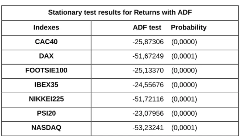
Table 3 - ADF test results for returns
Stationary test results for Returns with ADF Indexes ADF test Probability
CAC40 -25,87306 (0,0000) DAX -51,67249 (0,0001) FOOTSIE100 -25,13370 (0,0000) IBEX35 -24,55676 (0,0000) NIKKEI225 -51,72116 (0,0001) PSI20 -23,07956 (0,0000) NASDAQ -53,23241 (0,0001)
Note: The table includes the test value, and in brackets the probability associated to the
test.
Table 4 - KPSS test results for returns
Stationary test results for Returns with KPSS Indexes 5% level LM-statistic
CAC40 0,463000 (0,127395) DAX 0,463000 (0,218865) FOOTSIE100 0,463000 (0,195992) IBEX35 0,463000 (0,138946) NIKKEI225 0,463000 (0,156624) PSI20 0,463000 (0,199058) NASDAQ 0,463000 (0,314842)
Note: The table includes the critical value for a significance level of 5% and in brackets
the LM-statistic.
With the results, from the Augmented Dickey-Fuller test, we can see that the returns of the indexes analyzed are all stationary, because the probability associated to the test is lower than 0,05 (the confidence level considered by default), thus we reject (where a unit root is considered).
22 Considering the results from KPSS test we can also conclude that our indexes are all stationary because the LM-stat value is lower than the critical value considered for the significance level 5%, and due to that we don’t reject .
After computing the first differences of the log of prices as we obtained stationary series, we can now compute the Granger causality test and estimate the VAR models.
23
4.3 -
Granger causality test
As we have already discussed, if we have statistically significant values in Granger causality test we reject the null hypothesis, i.e, we assume that X Granger-causes Y.
On the Granger causality test we assume that current returns are influenced at maximum by returns of the two days before.
Table 5 present the results of Granger causality test, where the statistically significant values are highlighted.
Table 5 - Granger causality test for returns
Null Hypothesis: Obs F-Statistic Probability
DAX_RET does not Granger Cause CAC_RET 2513 27.4625 1.6E-12
CAC_RET does not Granger Cause DAX_RET 8.85040 0.00015
FOOTSIE_RET does not Granger Cause CAC_RET 2510 2.16606 0.11484
CAC_RET does not Granger Cause FOOTSIE_RET 0.16979 0.84385
IBEX_RET does not Granger Cause CAC_RET 2510 4.46122 0.01164
CAC_RET does not Granger Cause IBEX_RET 3.49386 0.03053
NASDAQ_RET does not Granger Cause CAC_RET 2513 106.880 2.9E-45
CAC_RET does not Granger Cause NASDAQ_RET 0.29321 0.74589
NIKKEI_RET does not Granger Cause CAC_RET 2510 0.58912 0.55489
CAC_RET does not Granger Cause NIKKEI_RET 156.418 9.7E-65
PSI20_RET does not Granger Cause CAC_RET 2510 4.30051 0.01366
CAC_RET does not Granger Cause PSI20_RET 2.24367 0.10628
FOOTSIE_RET does not Granger Cause DAX_RET 2510 1.06427 0.34514
DAX_RET does not Granger Cause FOOTSIE_RET 13.0676 2.3E-06
IBEX_RET does not Granger Cause DAX_RET 2510 1.71413 0.18033
DAX_RET does not Granger Cause IBEX_RET 6.57867 0.00141
NASDAQ_RET does not Granger Cause DAX_RET 2513 49.7117 6.7E-22
24
NIKKEI_RET does not Granger Cause DAX_RET 2510 0.81348 0.44343
DAX_RET does not Granger Cause NIKKEI_RET 181.285 3.0E-74
PSI20_RET does not Granger Cause DAX_RET 2510 1.88132 0.15260
DAX_RET does not Granger Cause PSI20_RET 2.16403 0.11508
IBEX_RET does not Granger Cause FOOTSIE_RET 2510 0.54065 0.58244
FOOTSIE_RET does not Granger Cause IBEX_RET 0.23991 0.78672
NASDAQ_RET does not Granger Cause FOOTSIE_RET 2510 96.7769 3.3E-41
FOOTSIE_RET does not Granger Cause NASDAQ_RET 0.24744 0.78082
NIKKEI_RET does not Granger Cause FOOTSIE_RET 2510 1.79379 0.16654
FOOTSIE_RET does not Granger Cause NIKKEI_RET 143.194 1.3E-59
PSI20_RET does not Granger Cause FOOTSIE_RET 2510 3.42077 0.03284
FOOTSIE_RET does not Granger Cause PSI20_RET 0.86442 0.42142
NASDAQ_RET does not Granger Cause IBEX_RET 2510 63.5960 1.1E-27
IBEX_RET does not Granger Cause NASDAQ_RET 1.42479 0.24075
NIKKEI_RET does not Granger Cause IBEX_RET 2510 0.17681 0.83795
IBEX_RET does not Granger Cause NIKKEI_RET 139.429 3.9E-58
PSI20_RET does not Granger Cause IBEX_RET 2510 1.92787 0.14567
IBEX_RET does not Granger Cause PSI20_RET 0.29196 0.74682
NIKKEI_RET does not Granger Cause NASDAQ_RET 2510 0.36719 0.69271
NASDAQ_RET does not Granger Cause NIKKEI_RET 266.418 1.E-105
PSI20_RET does not Granger Cause NASDAQ_RET 2510 2.74895 0.06419
NASDAQ_RET does not Granger Cause PSI20_RET 43.2697 3.4E-19
PSI20_RET does not Granger Cause NIKKEI_RET 2510 71.5671 5.9E-31
NIKKEI_RET does not Granger Cause PSI20_RET 6.91109 0.00102
As we can see in this test the probability associated with the F-test in DAX_RET does not Granger Cause CAC_RET, is 1.6E-12, thus lower than 0.05, which means that we reject in the Granger causality test. So past DAX returns help to forecast present CAC40 returns, the same happens on the opposite side, i.e., past CAC40 returns help to forecast present DAX returns, because the probability associated to the test is also lower than 0.05 (0.00015) thus we can conclude that there is a feedback between the two stocks returns. On the other hand when we are analyzing the probability associated with the F-test we observe that FOOTSIE_RET does not Granger cause CAC_RET, thus, we
25 see that the past returns of FOOTSIE100 will not help to forecast CAC40 returns, because its higher than 0.05 (0.11484) The same conclusion is verified when we analyze CAC_RET does not Granger Cause FOOTSIE_RET, because the probability associated to the test value is 0.84385.
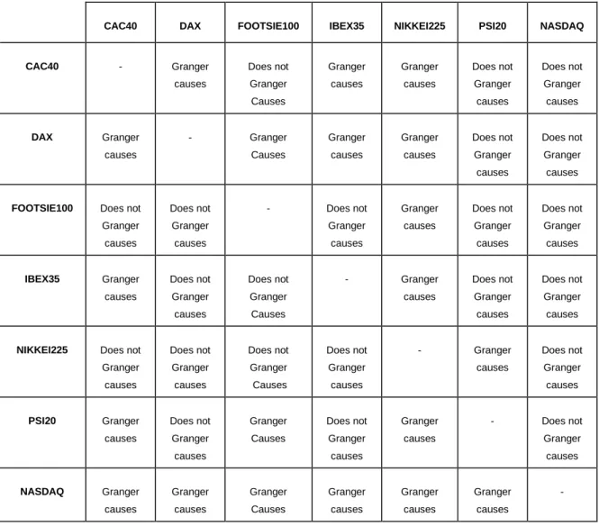
Following the criteria stated above, in table 6 we present the Granger causality results for the other stock indexes:
Table 6 - Granger causality test for returns (conclusion)
CAC40 DAX FOOTSIE100 IBEX35 NIKKEI225 PSI20 NASDAQ
CAC40 - Granger causes Does not Granger Causes Granger causes Granger causes Does not Granger causes Does not Granger causes DAX Granger causes - Granger Causes Granger causes Granger causes Does not Granger causes Does not Granger causes
FOOTSIE100 Does not Granger causes Does not Granger causes - Does not Granger causes Granger causes Does not Granger causes Does not Granger causes IBEX35 Granger causes Does not Granger causes Does not Granger Causes - Granger causes Does not Granger causes Does not Granger causes
NIKKEI225 Does not Granger causes Does not Granger causes Does not Granger Causes Does not Granger causes - Granger causes Does not Granger causes PSI20 Granger causes Does not Granger causes Granger Causes Does not Granger causes Granger causes - Does not Granger causes NASDAQ Granger causes Granger causes Granger Causes Granger causes Granger causes Granger causes -
26
4.4 - VAR Models
To estimate the VAR models we have defined as endogenous variables the returns of each index: CAC_RET, DAX_RET, FOOTSIE_RET and IBEX_RET, PSI20_RET and NASDAQ_RET, and as exogenous variables the past values (2 lags) of the same variables. The estimation sample, as already stated in the Data section, is associated with the period from 1st of January, 2000 to 31st of December, 2010. To define the lags we have estimated several VAR models and we noticed that as we increase the lags the Akaike Information Criterion shows slight decreases, contrary to Scharwz Criterion, and vice versa. Thus, we define the lags from 1 to 2. This seems an adjusted choice because it decreases the terms in the equation without compromising the final result (since the difference in the information criteria as we increase the lags is very tiny), and also because this way we keep the most recent observations.
Table 7 shows the results of the VAR model, where statistically significant values are highlighted. In the first part of the VAR model, three different types of values are presented: the estimation for the coefficients, the standard errors and the t-statistics. We define statistically significant values as those having a t-statistic absolute value (or modulus of t-statistic) higher than 2.
27
Table 7 - Results of VAR for returns
CAC_RET DAX_RET FOOTSIE_RET IBEX_RET NASDAQ_RET NIKKEI_RET PSI20_RET + CAC_RET(-1) -0.319768 -0.189902 -0.102611 -0.354271 0.001972 -0.022912 -0.220834 (0.06143) (0.06529) (0.05169) (0.06123) (0.08395) (0.05718) (0.04752) [-5.20518] [-2.90858] [-1.98523] [-5.78627] [ 0.02349] [-0.40070] [-4.64728] CAC_RET(-2) 0.058137 0.198932 0.036835 0.050970 -0.021847 0.190494 0.030347 (0.06121) (0.06505) (0.05150) (0.06100) (0.08364) (0.05 697) (0.04734) [ 0.94986] [ 3.05818] [ 0.71530] [ 0.83557] [-0.26119] [ 3.34383] [ 0.64101] DAX_RET(-1) 0.143364 -0.030043 0.091145 0.126738 0.115652 0.085841 0.089084 (0.04202) (0.04466) (0.03535) (0.04188) (0.05742) (0.03911) (0.03250) [ 3.41172] [-0.67272] [ 2.57801] [ 3.02624] [ 2.01398] [ 2.19474] [ 2.74073] DAX_RET(-2) -0.039700 -0.117307 -0.027843 -0.000573 0.015666 -0.015176 0.021704 (0.04187) (0.04450) (0.03523) (0.04173) (0.05721) (0.03897) (0.03238) [-0.94824] [-2.63635] [-0.79043] [-0.01372] [ 0.27381] [-0.38944] [ 0.67019] FOOTSIE_RET(-1) 0.075694 0.046350 -0.092629 0.102760 0.005098 0.131462 0.028376 (0.04951) (0.05262) (0.04165) (0.04934) (0.06766) (0.04608) (0.03830) [ 1.52892] [ 0.88090] [-2.22376] [ 2.08261] [ 0.07535] [ 2.85285] [ 0.74098] FOOTSIE_RET(-2) 0.030557 -0.023856 -0.029935 -0.014340 -0.006487 -0.042339 0.027111 (0.04912) (0.05220) (0.04133) (0.04895) (0.06712) (0.04572) (0.03799) [ 0.62213] [-0.45699] [-0.72436] [-0.29293] [-0.09665] [-0.92610] [ 0.71357] IBEX_RET(-1) -0.043768 0.021979 -0.048707 0.017999 -0.085623 0.085053 0.019013 (0.04481) (0.04762) (0.03770) (0.04466) (0.06123) (0.04171) (0.03466) [-0.97677] [ 0.46153] [-1.29195] [ 0.40305] [-1.39829] [ 2.03932] [ 0.54855] IBEX_RET(-2) -0.084054 -0.069380 -0.015373 -0.076505 0.010450 -0.078898 -0.072393 (0.04488) (0.04770) (0.03776) (0.04473) (0.06133) (0.04177) (0.03471) [-1.87293] [-1.45463] [-0.40713] [-1.71047] [ 0.17040] [-1.88880] [-2.08542] NASDAQ_RET(-1) 0.228078 0.185090 0.193910 0.184534 -0.062437 0.244703 0.126156 (0.01766) (0.01877) (0.01486) (0.01760) (0.02413) (0.01643) (0.01366) [ 12.9171] [ 9.86311] [ 13.0526] [ 10.4862] [-2.58756] [ 14.8893] [ 9.23674] NASDAQ_RET(-2) 0.064901 0.065567 0.047884 0.049431 -0.027151 0.013201 0.032466 (0.01870) (0.01987) (0.01573) (0.01863) (0.02555) (0.01740) (0.01446) [ 3.47107] [ 3.29950] [ 3.04380] [ 2.65262] [-1.06259] [ 0.75852] [ 2.24474] NIKKEI_RET(-1) -0.026756 -0.031602 -0.035589 -0.017098 -0.012540 -0.184757 -0.055365 (0.02331) (0.02478) (0.01962) (0.02324) (0.03186) (0.02170) (0.01803) [-1.14762] [-1.27538] [-1.81428] [-0.73585] [-0.39359] [-8.51382] [-3.06998] NIKKEI_RET(-2) -0.009628 -0.009495 -0.017100 0.008649 -0.011874 -0.011735 0.029514 (0.02132) (0.02266) (0.01794) (0.02125) (0.02914) (0.01985) (0.01649) [-0.45150] [-0.41897] [-0.95312] [ 0.40698] [-0.40745] [-0.59125] [ 1.78931] PSI20_RET(-1) -0.037136 -0.019399 -0.083422 -0.044293 -0.095003 -0.022201 0.062681 (0.03809) (0.04048) (0.03205) (0.03796) (0.05205) (0.03545) (0.02946) [-0.97499] [-0.47923] [-2.60319] [-1.16683] [-1.82521] [-0.62622] [ 2.12751] PSI20_RET(-2) -0.056233 -0.047331 -0.009077 -0.052551 0.016912 -0.051028 -0.055700 (0.03813) (0.04052) (0.03208) (0.03800) (0.05210) (0.03549) (0.02949) [-1.47489] [-1.16806] [-0.28297] [-1.38299] [ 0.32458] [-1.43792] [-1.88869] C -0.014787 0.004720 -0.003212 -0.004069 -0.022825 -0.019664 -0.015436 (0.03171) (0.03370) (0.02668) (0.03161) (0.04334) (0.02952) (0.02453) [-0.46630] [ 0.14004] [-0.12036] [-0.12874] [-0.52669] [-0.66618] [-0.62927] R-squared 0.093207 0.050910 0.092100 0.068579 0.009728 0.213234 0.058227 Adj. R-squared 0.088119 0.045584 0.087005 0.063353 0.004171 0.208819 0.052942 Sum sq. Resids 6283.218 7097.088 4447.831 6241.048 11734.05 5443.438 3759.403 S.E. equation 1.586923 1.686572 1.335177 1.581588 2.168646 1.477071 1.227508 F-statistic 18.31818 9.559548 18.07856 13.12165 1.750614 48.30060 11.01839 Log likelihood -4713.123 -4865.985 -4279.564 -4704.672 -5497.012 -4533.066 -4068.527 Akaike AIC 3.767429 3.889231 3.421963 3.760695 4.392042 3.623957 3.253807 Schwarz SC 3.802258 3.924060 3.456792 3.795523 4.426871 3.658786 3.288636 Mean dependent -0.014362 0.001290 -0.003610 -0.002563 -0.018866 -0.021260 -0.014971 S.D. dependent 1.661830 1.726379 1.397349 1.634201 2.173183 1.660594 1.261351 Determinant resid covariance (dof adj.) 1.529855
Determinant resid covariance 1.466993 Log likelihood -25411.68 Akaike information criterion 20.33202 Schwarz criterion 20.57582
28 From the first part of the VAR model we conclude the following:
For CAC40 returns, we found that the values of t-statistics associated with CAC_RET (-1), DAX_RET (-(-1), NASDAQ_RET (-(-1), and NASDAQ_RET (-2), are higher than 2 (in absolute values), which means that these observations are statistically relevant to explain the current value of CAC40. Consequently, we can conclude that the returns of CAC40, DAX, and NASDAQ with one lag and the returns of NASDAQ with two lags have impact on the current of CAC40 returns. The past returns of others variables do not explain the current value of the dependent variable once they have the absolute t-statistic value lower than 2.
For DAX returns, the values of t-statistics associated with CAC_RET (-1), CAC_RET (-2), DAX_RET (-2), NASDAQ (-1), and NASDAQ (-2)are higher than 2 (in absolute value) which means that the corresponding estimated coefficients are statistically significant. Consequently, we can conclude that the returns of CAC40, and NASDAQ with one lag and the returns of CAC40, and NASDAQ with two lags have impact on the present returns of DAX, and that DAX’s past returns with two lags are also useful in explaining their own present returns. The probabilities associated to the t-test of other variables are lower than 2 (in absolute values), so they do not explain the present of DAX_RET.
For FOOTSIE100 returns, we found that the values of t-statistics associated with DAX_RET (-1), FOOTSIE_RET (-1), NASDAQ_RET (-1), NASDAQ (-2), and PSI20_RET (-1) variables are higher than 2 (in absolute values), which means that these are statistically significant. Consequently, we can conclude that the returns of FOOTSIE100 can be impacted by its own returns and also by several other returns, such as, DAX, NASDAQ, and PSI20 with one lag, and by NASDAQ returns with two lags.
For IBEX35 returns, we can observe that the variables CAC_RET (-1), DAX_RET (-1), FOOTSIE_RET (-1), NASDAQ_RET (-1), and NASDAQ (-2), are statistically significant, i.e., CAC40, DAX, FOOTSIE and NASDAQ returns with one lag are able to influence the current returns of IBEX35, this is a situation that also happens with NASDAQ returns with two lags.
29 For NASDAQ returns we have only found two statistically significant values for the t-test, which means that from the seven indexes in analysis only the returns of DAX and NASDAQ itself with one lag have impact on NASDAQ current returns.
Considering now, the NIKKEI225 returns, we can observe that the values of t-statistics associated with CAC_RET (-2), DAX (-1), FOOTSIE (-1), IBEX_RET (-1), NASDAQ (-1), and the index’s own returns with one lag are statistically significant, because the variables are higher than 2 (in absolute values), so the returns of NASDAQ and NIKKEI225 with one lag and CAC40 returns with two lags have impact on current returns of NIKKEI225.
Finally, regarding the PSI20 returns we see that CAC_RET (-1), DAX_RET (-1), IBEX_RET (-2), NASDAQ_RET (-1), NIKKEI_RET (-1), and PSI20_RET (-1) with one lag, and IBEX_RET (-2) and also NASDAQ (-2), with two lags have influence on the current returns of PSI20.
Still related to the first part of the VAR model, we noticed that the returns of NASDAQ with one lag have impact in all the indexes current returns. Also, the returns of NASDAQ with two lags have impact in all indexes except on their own current returns and in NIKKEI225. The returns of FOOTSIE100, NIKKEI225, and PSI20 with two lags do not have impact in any current returns.
In the second part of the output, below the coefficient summary, we find standard OLS regression statistics for each equation.
Looking at R-Square, in the case of CAC40 returns, we can see that only 9.3207% of the dependent variable total variation is explained by the variation of the explanatory variables. The R-Square for the other indexes are 5.0910% for DAX returns, 9.2100% for FOOTSIE100 returns, 6.8579% for IBEX35 returns, and 5.8227% for PSI20. Though is still an insufficient value, NIKKEI225 is the index with the highest R-square value (21.3234%), while NASDAQ has the lowest with only 0.9728% of its returns (total variation) being explained by the variation on returns of the other indexes.
30 In the third part of the output, summary statistics for the VAR system as a whole are presented. The information criteria can be used for model selection, such as, determining the lag length of VAR, i.e., the model that present information criterion with smaller values is the preferred one.
Regarding the equation analysis from VAR models and, in order to observe the interaction on returns, we present a full example for the variable CAC_RET on table 8. Table 9 includes all variables.
To see a more detailed analysis you can see Appendices 1 and 2.
Table 8 - Interpretation of VAR equation for CAC_RET
Left side of
equation Right side of equation Interpretation
CAC_RET - 0.014787 In average terms, when all the others past stocks returns are zero, we expect a negative variation of 0.01% in CAC40 returns, assuming that the rest remains constant.
-0.319768*CAC_RET(-1) In average, when the CAC_ret from the day before increases by 1 pp the current returns from CAC decreases by -0.31%, assuming that the rest remains constant.
+0.143364*DAX_RET(-1) In average when DAX_ret from the day before increases by 1pp the current returns from CAC increases by 0.14%, assuming that the rest remains constant.
+0.075694*FOOTSIE_RET(-1)
In average when FOOTSIE_ret from the day before increases by 1pp the current returns from CAC increases by 0.07%, assuming that the rest remains constant.
- 0.043768 * IBEX_RET(-1) In average when IBEX_ret from the day before increases by 1pp the current returns from CAC decrease by 0.04%, assuming that the rest remains constant.
+ 0.228078*NASDAQ_RET(-1)
-0.026756*NIKKEI_RET(-1)
In average when NASDAQ_ret from the day before increases by 1 pp the current returns from CAC increases by 0.23%, assuming that the rest remains constant.
In average when NIKKEI_ret from the day before increases by 1pp the current returns from CAC decreases 0.03%, assuming that the rest remains constant.
- 0.037136 * PSI20_RET(-1) In average when PSI20_ret from the day before increases by 1pp the current returns from CAC decreases 0.04%, assuming that the rest remains constant.
31 + 0.058137 * CAC_RET(-2) In average when CAC_ret from the two days before increases by 1pp the
current returns from CAC increases 0.06%, assuming that the rest remains constant.
- 0.039700 * DAX_RET(-2) In average when DAX_ret from the two days before increases by 1pp the current returns from CAC decreases 0.04%, assuming that the rest remains constant.
+0.030557*FOOTSIE_RET(-2)
- 0.084054 * IBEX_RET(-2)
In average when FOOTSIE_ret from the two days before increases by 1pp the current returns from CAC increases 0.03%, assuming that the rest remains constant.
In average when IBEX_ret from the two days before increases by 1pp the current returns from CAC decreases 0.08%, assuming that the rest remains constant.
+0.064901*NASDAQ_RET(-2)
-0.009628*NIKKEI_RET(-2)
-0.056233* PSI20_RET(-2)
In average when NASDAQ_ret from the two days before increases by 1pp the current returns from CAC increases 0.06%, assuming that the rest remains constant.
In average when NIKKEI_ret from the two days before increases by 1pp the current returns from CAC decreases 0.01%, assuming that the rest remains constant.
In average when PSI20_ret from the two days before increases by 1pp the current returns from CAC decreases 0.06%, assuming that the rest remains constant.
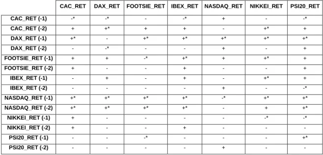
Table 9 – Signal and significance of the estimates in the VAR equations
CAC_RET DAX_RET FOOTSIE_RET IBEX_RET NASDAQ_RET NIKKEI_RET PSI20_RET CAC_RET (-1) -* -* - -* + - -* CAC_RET (-2) + +* + + - +* + DAX_RET (-1) +* - +* +* +* +* +* DAX_RET (-2) - -* - - + - + FOOTSIE_RET (-1) + + -* +* + +* + FOOTSIE_RET (-2) + - - + - - + IBEX_RET (-1) - + - + - +* + IBEX_RET (-2) - - - - + - -* NASDAQ_RET (-1) +* +* +* +* -* +* +* NASDAQ_RET (-2) +* +* +* +* - + +* NIKKEI_RET (-1) + - - - - -* -* NIKKEI_RET (-2) + - - + - - - PSI20_RET (-1) - - -* - - - +* PSI20_RET (-2) - - - - + - -
32 Through the table presented above we can conclude that the returns of NASDAQ from the day before and two days before have a positive and significant influence in the current returns of all the indices analyzed. The exception is when we analyze NASDAQ itself. In this case if we are considering the returns of the day before we have a significant and negative influence in the current returns of NASDAQ. However, if we are analyzing the returns from two days before we have a negative influence in the current returns of NASDAQ, but in this case is no longer significant.
33
5 - Conclusions
The main goal of this dissertation is to observe how some of the Capital Markets in the world interact among them, in order to test this interaction we used the Granger causality test, and the VAR methodology. The criterion used to choose the indices was based on the importance of the country to which the index belongs has to the world economy, in the Portugal case we decided to include this country in our analysis in order to observe which kind of behavior has the PSI20 against the most capital markets in the world.
Through the VAR methodology we can conclude that the returns from the day before on the American index NASDAQ have impact in the present returns of all the indexes analyzed including NASDAQ itself. The German index DAX follows the same pattern with only one exception the returns of the day before from DAX do not have impact on the present returns of DAX. In the opposite way we have NIKKEI225 and PSI20. The returns of these two markets are only influenced by returns of the day before from FOOTSIE100 and PSI20 itself, in the case of PSI20, and NIKKEI225 is influenced by NASDAQ and NIKKEI225 itself.
We can also observe that NASDAQ has a positive impact in all the other indexes, with only one exception NASDAQ itself. In this case current returns of NASDAQ have a negative influence on the returns from the day before and if we analyze the impact in returns from two days before we also observe a negative influence. However in this case is not statistically significant.
Regarding the Granger causality test we can also observe that NASDAQ returns granger cause the returns from all of the other indexes, i.e., the past returns from NASDAQ help to forecast the current returns from all of the indexes analyzed, we observe that the opposite happens when analyze if any of the other returns Granger cause NASDAQ returns, i.e., none of the past returns from all of the other indexes analyzed help to forecast the current returns of NASDAQ.
34 We can also conclude that FOOTSIE returns only Granger cause the returns of NIKKEI, and NIKKEI returns only Granger cause the returns of PSI20.
As future guidelines we suggest that a similar study should be done considering the markets analyzed in this dissertation, the major difference would be the frequency of the observations, i.e, we suggest that in future researches a database with weekly or monthly observations should be used, in order to check if the main conclusions from this thesis is still observed or not.
35
References
Edwards, S., (1998), “Interest Rate Volatility, Contagion and Convergence: An
Empirical Investigation of the cases of Argentina, Chile, and Mexico”, Journal of
Applied Economics, Vol I, Nº .1, pp 55-86
Nagayasu, J., (2000), “Currency Crisis and Contagion: Evidence from Exchange Rates
and Sectoral Stock Indices of the Philippines and Thailand”, International Monetary
Fund Working Paper
Bazdresch, S., and Werner, A., (2000), “Contagion of International Financial Crises:
The case of Mexico”, Dirección General de Investigación Económica
Caiado, J., (2002), “Modelos VAR, Taxas de Juro e Inflação”, Actas do 10th Portuguese Statistical Society Conference, pp 215-228
Yang, T., and Lim, J., (2004), “Crisis, Contagion, and East Asian Stock Markets”, World Scientific Publishing Co. and Center for PBBEF Research, Vol.7, Nº .1, pp 119-151
Dias, J., and Assis L., (2005), “ O impacto da política fiscal e do nível tecnológico
sobre o crescimento económico no Brasil: 1951/2000”, Cad. Fin. Públ., Brasília, Nº .6,
pp 5-59
Shachmurove, Y., (2005), “Dynamic Linkages Among the Emerging Middle Eastern
and the United States Stock Markets”, International Journal of Business
Cheong, C., Tesfa M., and Vaughan Williams, L. (2006), “Dynamic Links Between
Unexpected Exchange Rate Variation, Prices, and International Trade”, Open
36 Lin, C., Huang, C., and Wu, Y. (2008), “Effect of Market Imperfection on the
Relationship between future index prices and spot interest returns: An Empirical study”, International Journal of Management, Vol.25 Nº .2, pp 247-261
Laopodis, N. (2009), “REITs, the stock market and economic activity”, Journal of Property Investment & Finance, Vol. 27, Nº .6, pp 563-578
Guidi, F. (2010), “The Economic Effects of Oil Prices Shocks on the UK Manufacturing
and Services Sectors”, IUP
Zeaiter, H. (2010), “The Effect of Pre 2007-2008 Imported Crude Oil Prices Increases
on U.S. Economy”, The Business Review, Cambridge, Vol. 16, Nº .2
Ndaka, U. (2010), “Financial Development and Economic Growth: Evidence from
Nigeria”, IUP
Tsay, R. (2005), “Analysis of Financial Time Series”, A. John Wiley & Sons, Inc. Publication;
Robalo Marques, C. (1998), “Dynamic Models, Unit Roots, and Cointegration”, Edinova, Universidade Nova de Lisboa;
37
Appendix
38
Appendix 1 - VAR equations obtained from the estimated output
In this appendix we present the equations obtained from the estimated output.
Equation for CAC returns
- 0.014787 - 0.319768 * CAC_RET(-1) + 0.143364 * DAX_RET(-1) + 0.075694 * FOOTSIE_RET(-1) - 0.043768 * IBEX_RET(-1) + 0.228078 * NASDAQ_RET(-1) -0.026756 * NIKKEI_RET(-1) - 0.037136 * PSI20_RET(-1) + 0.058137 * CAC_RET(-2) - 0.039700 * DAX_RET(-2) + 0.030557 * FOOTSIE_RET(-2) - 0.084054 * IBEX_RET(-2) + 0.064901 * NASDAQ_RET(-2) - 0.009628 * NIKKEI_RET(-2) - 0.056233 * PSI20_RET(-2)
Equation for DAX returns
0.004720 - 0.189902 * CAC_RET(-1) - 0.030043 * DAX_RET(-1) + 0.046350 * FOOTSIE_RET(-1) + 0.021979 * IBEX_RET(-1) + 0.185090 * NASDAQ_RET(-1) - 0.031602 * NIKKEI_RET(-1) - 0.019399 * PSI20_RET(-1) + 0.198932 * CAC_RET(-2) - 0.117307 * DAX_RET(-2) - 0.023856 * FOOTSIE_RET(-2) - 0.069380 * IBEX_RET(-2) + 0.065567 * NASDAQ_RET(-2) - 0.009495 * NIKKEI_RET(-2) - 0.047331 * PSI20_RET(-2)
Equation for Footsie100 returns
- 0.003212 - 0.102611 * CAC_RET(-1) + 0.091145 * DAX_RET(-1) - 0.092629 * FOOTSIE_RET(-1) - 0.048707 * IBEX_RET(-1) + 0.193910 * NASDAQ_RET(-1) - 0.035589 * NIKKEI_RET(-1) - 0.083422 * PSI20_RET(-1) + 0.036835 * CAC_RET(-2) - 0.027843 * DAX_RET(-2) - 0.029935 * FOOTSIE_RET(-2) - 0.015373 * IBEX_RET(-2) + 0.047884 * NASDAQ_RET(-2) - 0.017100 * NIKKEI_RET(-2) - 0.009077 * PSI20_RET(-2)
Equation for Ibex35 returns
- 0.004069 - 0.354271 * CAC_RET(-1) + 0.126738 * DAX_RET(-1) + 0.102760 * FOOTSIE_RET(-1) + 0.017999 * IBEX_RET(-1) + 0.184534 * NASDAQ_RET(-IBEX_RET(-1) - 0.017098 * NIKKEI_RET(-IBEX_RET(-1) - 0.044293 * PSI20_RET(-IBEX_RET(-1) + 0.050970 * CAC_RET(-2) - 0.000573 * DAX_RET(-2) - 0.014340 * FOOTSIE_RET(-2) - 0.076505 * IBEX_RET(-2) + 0.049431 * NASDAQ_RET(-2) + 0.008649 * NIKKEI_RET(-2) - 0.052551 * PSI20_RET(-2)
Equation for NASDAQ returns
- 0.022825 + 0.001972 * CAC_RET(-1) + 0.115652 * DAX_RET(-1) + 0.005098 * FOOTSIE_RET(-1) - 0.085623 * IBEX_RET(-1) -0.062437 * NASDAQ_RET(-IBEX_RET(-1) - 0.012540 * NIKKEI_RET(-IBEX_RET(-1) - 0.095003 * PSI20_RET(-IBEX_RET(-1) - 0.021847 * CAC_RET(-2) + 0.015666 * DAX_RET(-2) - 0.006487 * FOOTSIE_RET(-2) + 0.010450 * IBEX_RET(-2) -0.027151 * NASDAQ_RET(-2) - 0.011874 * NIKKEI_RET(-2) + 0.016912 * PSI20_RET(-2)
Equation for Nikkei225 returns
- 0.019664 - 0.022912 * CAC_RET(-1) + 0.085841 * DAX_RET(-1) + 0.131462 * FOOTSIE_RET(-1) + 0.085053 * IBEX_RET(-1) + 0.244703 * NASDAQ_RET(-IBEX_RET(-1) - 0.184757 * NIKKEI_RET(-IBEX_RET(-1) - 0.022201 * PSI20_RET(-IBEX_RET(-1) + 0.190494 * CAC_RET(-2) - 0.015176 * DAX_RET(-2) - 0.042339 * FOOTSIE_RET(-2) - 0.078898 * IBEX_RET(-2) + 0.013201 * NASDAQ_RET(-2) - 0.011735 * NIKKEI_RET(-2) - 0.051028 * PSI20_RET(-2)
Equation for Psi20 returns
- 0.015436 - 0.220834 * CAC_RET(-1) + 0.089084 * DAX_RET(-1) + 0.028376 * FOOTSIE_RET(-1) + 0.019013 * IBEX_RET(-1) + 0.126156 * NASDAQ_RET(-IBEX_RET(-1) - 0.055365 * NIKKEI_RET(-IBEX_RET(-1) + 0.062681 * PSI20_RET(-IBEX_RET(-1) + 0.030347 * CAC_RET(-2) +
39 0.021704 * DAX_RET(-2) + 0.027111 * FOOTSIE_RET(-2) - 0.072393 * IBEX_RET(-2) + 0.032466 * NASDAQ_RET(-2) + 0.029514 * NIKKEI_RET(-2) – 0.055700 * PSI20_RET(-2)
Appendix 2 - Equations interpretation of VAR models
In this appendix we present an interpretation of the equations obtained through the VAR test, excluding the variable CAC_RET that is already stated on table 8.
Left side of
equation Right side of equation Interpretation
DAX_RET 0.004720 In average terms, when all the others past stocks returns are zero, we expect a positive variation of 0.005% in Dax returns, assuming that the rest remains constant.
-0.189902*CAC_RET(-1) In average when CAC_ret from the day before increases by 1pp the current returns from Dax decreases 0.19%, assuming that the rest remains constant.
-0.030043*DAX_RET(-1) In average when DAX_ret from the day before increases by 1pp the current returns from Dax decreases 0.03%, assuming that the rest remains constant.
+0.046350*FOOTSIE_RET(-1)
In average when FOOTSIE_ret from the day before increases by 1pp the current returns from Dax increases 0.05%, assuming that the rest remains constant.
+0.021979*IBEX_RET(-1) In average when IBEX_ret from the day before increases by 1pp the current returns from Dax increases 0.02%, assuming that the rest remains constant.
+0.185090*NASDAQ_RET(-1)
-0.031602*NIKKEI_RET(-1)
In average when NASDAQ_ret from the day before increases by 1pp the current returns from Dax increases 0.19%, assuming that the rest remains constant.
In average when NIKKEI_ret from the day before increases by 1pp the current returns from Dax decreases 0.03%, assuming that the rest remains constant.
-0.019399*PSI20_RET(-1) In average when PSI20_ret from the day before increases by 1pp the current returns from Dax decreases 0.02%, assuming that the rest remains constant.
+0.198932*CAC_RET(-2) In average when CAC_ret from the two days before increases by 1pp the current returns from Dax increases 0.20%, assuming that the rest remains constant.
-0.117307*DAX_RET(-2) In average when DAX_ret from the two days before increases by 1pp the current returns from Dax decreases 0.12%, assuming that the rest remains constant.
40 - 0.069380 * IBEX_RET(-2)
current returns from Dax decreases 0.02%, assuming that the rest remains constant.
In average when IBEX_ret from the two days before increases by 1pp the current returns from Dax decreases 0.07%, assuming that the rest remains constant.
+0.065567*NASDAQ_RET(-2)
-0.009495*NIKKEI_RET(-2)
-0.047331*PSI20_RET(-2)
In average when NASDAQ_ret from the two days before increases by 1pp the current returns from Dax increases 0.07%, assuming that the rest remains constant.
In average when NIKKEI_ret from the two days before increases by 1pp the current returns from Dax decreases 0.009%, assuming that the rest remains constant.
In average when PSI20_ret from the two days before increases by 1pp the current returns from Dax decreases 0.05%, assuming that the rest remains constant.
Left side of
equation Right side of equation Interpretation
FOOTSIE_RET -0.003212 In average terms, when all the others past stocks returns are zero, we expect a negative variation of 0.003% in Footsie returns, assuming that the rest remains constant.
-0.102611* CAC_RET(-1) In average when FOOTSIE_ret from the day before increases by 1pp the current returns from Footsie100 decreases by 0.10%, assuming that the rest remains constant.
+0.091145*DAX_RET(-1) In average when DAX_ret from the day before increases by 1pp the current returns from Footsie100 increases by 0.09%, assuming that the rest remains constant.
-0.092629*FOOTSIE_RET(-1)
In average when FOOTSIE_ret from the day before increases by 1pp the current returns from Footsie100 decreases by 0.09%, assuming that the rest remains constant.
-0.048707*IBEX_RET(-1) In average when IBEX_ret from the day before increases by 1pp the current returns from Footsie100 decreases by 0.05%, assuming that the rest remains constant.
+0.193910*NASDAQ_RET(-1)
-0.035589*NIKKEI_RET(-1)
In average when NASDAQ_ret from the day before increases by 1pp the current returns from Footsie100 increases by 0.19%, assuming that the rest remains constant.
In average when NIKKEI_ret from the day before increases by 1pp the current returns from Footsie100 decreases by 0.04%, assuming that the rest remains constant.
-0.083422*PSI20_RET(-1) In average when PSI20_ret from the day before increases by 1pp the current returns from Footsie100 decreases by 0.08%, assuming that the rest remains constant.