Reginaldo Antonio Medeiros , Haroldo Nogueira de Paiva , Flávio Siqueira D’Ávila and Helio Garcia Leite
(1)Instituto Federal de Educação, Ciência e Tecnologia de Mato Grosso, Campus Cáceres, Prof. Olegário Baldo, Avenida dos Ramires, s/no, Caixa Postal 244, CEP 78200-000 Cáceres, MT, Brazil. E-mail: reginaldo.medeiros@cas.ifmt.edu.br (2)Universidade Federal de Viçosa, Departamento de Engenharia Florestal, Avenida Purdue, s/no, Campus Universitário, Edifício Reinaldo de Jesus Araújo, CEP 36570-900 Viçosa, MG, Brazil. E-mail: hnpaiva@ufv.br, hgleite@gmail.com (3)Companhia do Vale do Araguaia, Fazenda São Jorge, Rodovia MT 240, Km 23, Zona Rural, CEP 78635-000 Água Boa, MT, Brazil. E-mail: fdavila@valedoaraguaia.com.br
Abstract – The objective of this work was to evaluate the growth and yieldofteak (Tectona grandis) stands at different spacing and in different soil classes. Twelve spacing were evaluated in an Inceptisol and Oxisol, in plots with an area of 1,505 or 1,548 m2, arranged in a completely randomized design with nine replicates. The
teak trees were measured at 26, 42, 50, and 78 months of age. Total tree height was less affected by spacing. Mean square diameter was greater in wider spacing, whereas basal area and total volume with bark were greater in closer spacing. An increase in volume with bark per tree was observed with the increase of useful area per plant. For teak trees, growth stagnation happens earlier, the growth rate is higher in closer spacing, and the plants grow more in the Inceptisol than in the Oxisol.
Index terms: Tectona grandis, initial spacing, modeling.
Crescimento e produção de povoamentos de teca em diferentes espaçamentos
Resumo – O objetivo deste trabalho foi avaliar o crescimento e a produção de povoamentos de teca (Tectona grandis) em diferentes espaçamentos e classes de solo. Foram avaliados 12 espaçamentos em Cambissolo e Latossolo, dispostos em parcelas com área de 1.505 ou 1.548 m2, em delineamento inteiramente casualizado,
com nove repetições. As plantas de teca foram medidas aos 26, 42, 50 e 78 meses de idade. A altura total das árvores foi menos influenciada pelos espaçamentos. O diâmetro quadrático médio foi superior nos maiores espaçamentos, enquanto a área basal e o volume total com casca foram superiores nos espaçamentos mais adensados. Observou-se aumento do volume com casca por árvore com o aumento da área útil por planta. Em teca, a estagnação do crescimento ocorre mais cedo, a taxa de crescimento é maior nos espaçamentos mais adensados e as plantas crescem mais em Cambissolo do que em Latossolo.
Termos para indexação: Tectona grandis, espaçamento inicial, modelagem.
Introduction
Teak (Tectona grandis L.f.), belonging to the
botanical family Lamiaceae (ex Verbenaceae), is native to tropical forests of Southeast Asia, including India, Myanmar, Thailand, and Laos, and is considered a noble species because of its high commercial value, stability, workability, strength, and natural durability (Reis & Paludzyszyn Filho, 2011). It is one of the main forest species cultivated worldwide, with a planted area of 6,887 million hectares in 2015 (Midgley et al., 2015). In Latin America, the largest planted area of 87,502 ha is found in Brazil (Ibá, 2017), where the state of Mato Grosso is the main producer.
The adaptation of teak to the edaphic and climatic conditions of Mato Grosso and the international value of wood has led to the recent expansion of the culture in the state. However, rather than increasing the
planted area, there is now a concern to increase crop productivity, especially through the selection of more productive genotypes, appropriate sites, and adequate management practices. Among management practices, the definition of initial plant spacing stands out.
which is very responsive to environmental conditions and to the management to which it is subjected to (Pelissari et al., 2014a; Medeiros, 2016).
In Brazil, several studies have been carried out to assess the effects of spacing on teak cultivation (Macedo et al., 2005; Rondon, 2006; Lima et al., 2009; Silva et al., 2016). However, these works have not addressed variations in plant spacing, which affect the quantitative and qualitative development of plant individuals and populations (Medeiros, 2016), causing problems related to productivity (Silva et al., 2016), technological properties of wood (Zahabu et al., 2015), handling regime (Pelissari et al., 2014a; Paiva & Leite, 2015), nutrition (Behling et al., 2014), and operational costs and yields (Pelissari et al., 2014a).
In addition, few known researches have evaluated teak development as affected by the productive capacity of the site (soil), which is defined as the potential of a given species or clone for the production of wood or another product in a given area (Oliveira et al., 2008). It should be noted that teak often presents growth and yield problems when grown in compacted, poorly-drained, shallow, and acidic soils with low natural fertility (Behling et al., 2014; Pelissari et al., 2012, 2014a; Midgley et al., 2105; Medeiros, 2016).
The objective of this work was to evaluate the growth and yield of teak stands at different spacing and in different soil classes.
Materials and Methods
The data used in the study were obtained from two experiments on spacing in teak plantations carried out in the municipality of Água Boa, in the eastern region of the state of Mato Grosso, Brazil. The experiments were established in 2009, in two sites at the following geographic coordinates, respectively: 13°59'54"S, 52°24'51"W, at 368 m altitude; and 14°00'33"S, 52°24'34"W, at 378 m altitude.
The climate of the region is of the Aw type – tropical, with a rainy summer from October to April and a dry winter from May to September –, with annual rainfall varying from 1,800 to 2,200 mm. In site 1, the soil is classified as a Cambissolo Háplico Tb distrófico (alumínico) endopetroplíntico, i.e., the Inceptisol haplic cambisol dystrophic Tb, with flat to gently undulated relief; and in site 2, as a Latossolo Vermelho distrófico típico, i.e., the Oxisol typical dystrophic, with flat to gently undulating relief (Table 1). In each experiment, 12 spacing were evaluated: 5.0×1.5, 3.5×2.2, 3.5×2.4, 3.5×2.6, 3.5×2.8, 4.0×3.0, 5.0×3.0, 4.0×4.0, 6.0×3.0, 5.0×4.0, 0.0×4.0, and 5.0×5.0 m, arranged in a completely randomized design, with nine replicates. The experimental units were composed of plots with
an area of 1,505 or 1,548 m2, totaling 18.48 ha in each
experiment.
The Inceptisol was prepared by ripping and subsoiling at the depths of 90 to 110 cm, which presented physical impediments (Santos et al., 2013), and the Oxisol by subsoiling at 45 to 50 cm. Seminal seedlings of teak were used, produced in tubes with a
capacity of 115 cm3. Planting was carried out manually,
and replanting was performed 40 days later. On this
occasion, 170 g N-P2O5-K2O (6:30:6) fertilizer were
applied per plant.
The control of invasive plants was accomplished by manual weeding (crowning), chemical weeding by applying the glyphosate herbicide between the lines and in the lines in wider spacing, and semi-mechanized mowing in the line and mechanized mowing between the lines. One year after planting, thinning was carried out.
The trees in the experimental plots were measured at 26, 42, 50, and 78 months after planting. At 26 and 42 months of age, the total height of the first ten trees of the plots was measured, and at 50 and 78 months the heights of the first five trees. The height of the other
Table 1. Chemical and physical characteristics of the soils of the experimental area.
Soil(1) Depth
(cm)
Ca Mg Ca+Mg Al H+Al K P-Mehlich S Zn SOM BS pH (H2O)
---(cmolc dm-3)--- --- (mg dm-3)---
---(%)---CXb2fd 0–20 1.7 0.45 2.15 0.65 2.3 34 162.2 0 1.3 1.3 46.7 5.4 20–40 1.6 0.75 2.3 0.6 2.7 30 14 0 1.1 1.05 47.0 5.2 LVd4d 0–20 1.6 1.05 2.65 0.35 4.15 52.5 7.35 0 2.05 1.55 40.1 5.5 20–40 0.9 0.6 1.45 0.65 4.2 28 4.7 0 1.95 1.35 26.4 5.2
(1)CXb2fd, Cambissolo Háplico Tb distrófico (alumínico) endopetroplíntico, an Inceptisol; and LVd4d, Latossolo Vermelho distrófico típico, an Oxisol.
trees was estimated by hypsometric relation (simple linear equation) – one for each soil class. The diameter of all trees was measured at 1.3 m height.
At 64 months, no measurements were performed in the field, and tree diameter and total height for each spacing and site were estimated using the equations obtained from the data available for the other ages, by adjusting the model of Piennar & Shiver (1981), according to the following equation:
y2=y1×exp
(
−α(
I2−I1)
)
+εβ β
where y is the total diameter or height in the current
(1) and future (2) ages (I); α and β are the model’s parameters; and ɛ is the random error. In all spacing
and sites evaluated, the parameters of the adjusted
equations were significant and the corresponding coefficients of correlation were higher than 95%.
The volume with bark was estimated by the company Companhia do Vale do Araguaia that owns the experimental area, using the Schumacher & Hall (1933) model.
To evaluate the effect of spacing on teak plants, the last measurement was taken at 78 months, which was considered the age of interest. For this, the analysis of variance was used, and, when significant, the means of the variables total height, mean square diameter, basal area, volume with bark, and survival were compared
using Tukey’s test, at 5% probability.
However, considering that it is possible to analyze data at a single age using the analysis of variance and the means test and over ages with modeling, the Gompertz model was adjusted to assess the growth trend for total height, mean square diameter, basal area per hectare, and volume with bark per hectare as affected by spacing, using the equation:
y=β0×exp (exp(− β1−β2I)+ε
where y is the variable considered at age I, β is the model’s parameter, and ɛ is the random error.
The model was adjusted for spacing and soil class, and the obtained equations were compared by model identity tests (Regazzi & Silva, 2010). For this, the following equation, under normal conditions, was used:
F n k Y Y Y Y
i j ij ij r i j ij ij c
=( − )×
(
−)
−(
−)
∑
∑
∑ ∑
1 2 2 . , . , k1 k2 i j Yij Yij c F K K and n K
2
1 2 1
−
( )×
∑ ∑
.(
− ,)
~ ( ;( − )) ( − )
α
degrees of freedom, where Ŷij,r is the jth estimated
observation of a Y variable of a reduced model, and
Ŷij,c is the jth estimated observation of a Y variable of a
complete model. In this case, Yji is the jth observation
of a Y variable in a i data set, where i = 1, 2, ..., H and j = 1, 2, ..., ni, where n i ni
H
=
=
∑
;1 and K1 and K2 are
the number of coefficients in a complete and reduced
model, respectively, for a H0 hypothesis (identity
hypothesis). Since the equations of the Gompertz model were compared two-by-two in the present study, H = 2, K1 = 6 (six coefficients), and K2 = 3 (three
coefficients).
The adjusted equations were evaluated based on
the coefficient of correlation (Ryŷ), residual standard
error (Syx), and graphical analysis of the percentage of
relative errors (ER), through the respective equations:
R n y y y y
n y y n
yy i i m i
n i m i n =
(
( − )( − ))
− ( )(
)
− = − =∑
∑
1 1 1 2 1 −− = − = = − ( )(
)
= = ( − ) − −∑
∑
∑
1 2 1 1 1 2 1 1y y y n y
S y y n p
E
i i n
m i i
n
yx i i i
n
;
R
R%=100((yI−yi) yi)
where yi and ŷi, respectively, are the observed and
estimated values of the dependent variable of interest; x is the independent variable; i is the ith observation of
the variable of interest; y̅ is the arithmetic mean of y;
ŷm is the mean of the estimates of y; n is the number
of observations; and p is the number of independent variables in the model.
Results and Discussion
At 78 months of age, regardless of the experimental site, spacing affected the variables mean height, mean square diameter, basal area, bark volume, and survival. Of these, mean height was the least affected (Figure 1), since trees with the greatest and lowest average heights were observed both in wider (5.0×5.0 and 6.0×3.0 m, respectively) and closer (3.5×2.8 and 5.0×1.5 m) spacing in the Inceptisol; similar results were found for the Oxisol.
The lowest average tree height at 78 months of age in both sites was verified at the 5.0×1.5 m spacing, considered the closest. Zahabu et al. (2015) found similar results when studying the effect of 2×2, 3×3, and 4×4 m spacing on the production and properties of teakwood in Tanzania. In the present work and in that of Zahabu et al. (2015), the lowest height was attributed to the competition among plants and to the productive capacity of the site, as also reported by Forrester et al. (2010) and Medeiros et al. (2017).
As the useful area per plant increased, there was a greater increase in mean diameter, but a reduction in total basal area and volume with bark. According to other studies on several forest species (Leite et al., 2006; Lima et al., 2009; Chotchutima et al., 2013; Zahabu et al., 2015; Silva et al., 2016), mean square diameter, basal area, and volume with bark were also affected by the same spacing assessed in the present work. Silva et al. (2016) evaluated the spacing of 3×2, 4×2, 5×2, 6×2, 3×2×2, 4×2×2, 5×2×2, and 6×2×2 m in teak populations at 192 months of age, and concluded that the lower the density of trees, the larger the
diameter, and the higher the density, the greater the basal area and the volume with bark per hectare.
The decrease in total volume from the closer to the wider spacing (Figure 1) is due to the number of individuals and the shape of the tree trunks. For the same diameter and total height, closer spacing resulted in greater volume (Nogueira et al., 2008), because the trees had a less conical trunk than in the wider spacing (Forrester et al., 2010).
Although the volume with bark per hectare was greater at the closer spacing of 5.0×1.5, 3.5×2.2, 3.5×2.4, and 3.5×2.8 m because of a greater number of individuals (Figure 1), the individual tree volume was lower (Figure 2), which was attributed to a smaller diameter, as also found by Paiva & Leite (2015) and Silva et al. (2016). In the spacing of 3.5×2.4 m, the average volume with bark was 93.01±4.42 and
91.39±7.10 m3 ha-1 in the Inceptisol and Oxisol,
respectively. That is, 49 and 44% higher than the volume with bark of 47.70±6.54 and 51.06±14.32
m3 ha-1 observed in the 6×4 m spacing for each soil
class, respectively. Moreover, the individual volume
Figure 1. Total height, mean square diameter, basal area per hectare, volume with bark per hectare, number of individuals
per hectare, and survival of teak (Tectona grandis) at 78 months of age in an Inceptisol (CXb2fd) and in an Oxisol
with bark in the 6×4 m spacing was 0.143±0.009 and
0.131±0.029 m3 per plant, in the Inceptisol and Oxisol,
respectively, which was 36 and 38% higher than the
individual volume of 0.131±0.0029 and 0.081±0.006 m3
per plant in the 3.5×2.4 m spacing for these same soils. Depending on the purpose of the wood, the total usable volume is more important than the total volume produced. However, very wide spacing can lead to the sub-occupation of the growing space and to a lower final production than that in the closer spacing. In this respect, optimal spacing is considered as the one capable of producing maximum wood regarding size, shape, and quality, at the lowest cost.
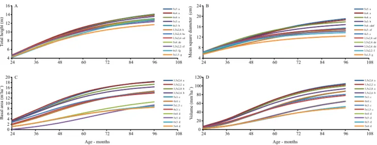
During rotation (Figures 3 and 4), it was observed that spacing affected all studied variables, with a less
significant effect on total height, showing that teak is sensitive to intraspecific competition (Caldeira & Oliveira, 2008; Pelissari et al., 2013). In the closer spacing, due to a higher demand for nutrients, water, and solar radiation, there may be a reduction in the number of buds, in the size of branches, and in the production of leaves (Forrester et al., 2010; Chotchutima et al., 2013). It should be pointed out that, although essential to explain growth and production, the effect of spacing on plant physiology was not assessed in the present study, indicating the need for new researches on the topic.
In the Inceptisol, the adjusted equations of the Gompertz model used to evaluate growth and production trends as affected by age showed, in most cases, a correlation coefficient above 90% and a low standard error among the dependent (total height, mean square diameter, basal area per hectare, and volume with bark per hectare) and independent (age) variables. The exception were the variables basal area and volume with bark at the spacing of 5.0×1.5 and 6.0×3.0 m, which presented lower statistics of accuracy and precision (Table 2). In the Oxisol, the lowest accuracies were obtained at the spacing of 5.0×1.5, 6.0x3.0, and 5.0×4.0 m, where lower survival rates of 86, 86, and 88% (Figure 1), respectively, were observed due to plant competition (Forrester et al.,
Figure 2. Average volume with bark (Vcc) per teak
(Tectona grandis) plant at different spacing and in different soil classes at 78 months of age. Within a single soil class, averages followed by equal letters do not differ from each
other by Tukey’s test, at 5% probability.
Figure 3. Growth trend for total height (A), mean square diameter (B), basal area per hectare (C), and volume with bark per
hectare (D) of teak (Tectona grandis) according to the plant spacing and ages evaluated in an Inceptisol (CXb2fd). Equal letters for each variable among treatments indicate equality in the growth trend by the F-test for model identity. CXb2fd,
Cambissolo Háplico Tb distrófico (alumínico) endopetroplíntico.
a a
b b bc
cd de
def ef
efg fg g
a a
a
ab
bc bcd bc bc bcd
bcd cd
d
0.00 0.05 0.10 0.15 0.20
5x5 6x4 4x4 5x3 5x4 6x3 4x3 3.5x2.8 3.5x2.4 3.5x2.6 3.5x2.2 5x1.5
Vcc (m plant
)
3
-1
2010) and the productive capacity of the site (Pelissari et al., 2014a).
The values of the asymptotes, i.e., β0 parameters of
the Gompertz model, were close to the mean values projected by the model for total height at 96 months (Table 2), which suggests that growth stagnation is imminent, regardless of spacing. This finding is more evident for mean square diameter, basal area per hectare, and volume with bark per hectare, which are more affected by spacing. For these variables, the asymptotic values and those projected by the 96-month model showed greater proximity at closer spacing (3.5×2.2, 3.5×2.4, 3.5×2.6, 3.5×2.8, and 4.0×3.0 m) than at wider spacing (5×3, 4.0×4.0, 6.0×3.0, 5.0×4.0, 6.0×40, and 5.0×5.0 m), indicating that growth stagnation is nearer (Leite et al., 2006).
For the same spacing, the asymptotes of the equations (Table 2), as well as mean square diameter (Figure 1) and average volume with bark per plant (Figure 2), were greater for teak grown in the Inceptisol than in the Oxisol. Although the Inceptisol is more restrictive to teak cultivation (Medeiros, 2016) due to the occurrence of rock fragments in the soil mass (Santos et al., 2013), plant growth can be benefited by the nutrient reserves present in the soil, as observed by Tonini et al. (2009) and Medeiros et al. (2015). In
addition, teak requires soils with higher phosphorus content and base saturation (Favare et al., 2012), and does not tolerate the presence of hydrogen and aluminum (Pelissari et al., 2014a, 2014b), which were found in the Inceptisol evaluated in this work (Table 1).
The growth rates for all variables, i.e., β2 parameters
of the Gompertz model (Table 2), were higher in the closer spacing than in the wider ones. This result may be due to a greater leaf area index in higher population densities, which allows canopies to intercept more light, increasing the efficiency in the use of the available resources, such as water, nutrients, and radiation, per area unit (Chotchutima et al., 2013). This allows for greater mass production at early ages; however, the production capacity of the site is reached faster, requiring earlier forestry interventions, such as thinning (Paiva & Leite, 2015).
The results obtained in the present study show the importance of monitoring the growth and production of a forest population, in order to determine the best time for the application of forestry practices aiming to avoid growth stagnation, especially for species with higher rotation, such as teak, and that require periodical forestry interventions, including stripping and thinning. The importance of using modeling in the analysis of experimental data on tree spacing was
Figure 4. Growth trend for total height (A), mean square diameter (B), basal area per hectare (C), and volume with bark per
hectare (D) of teak (Tectona grandis) according to the plant spacing and ages evaluated in an Oxisol (LVd4d). Equal letters for each variable among treatments indicate equality in the growth trend by the F-test for model identity. LVd4d, Latossolo
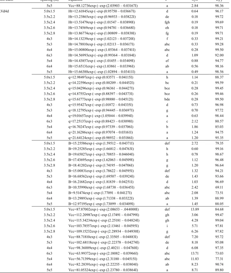
Table 2. Gompertz model parameters adjusted for the variables total height (Ht), mean square diameter (q), basal area (B), and volume with bark (Vcc) for teak planted in an Inceptisol (CXb2fd) and in an Oxisol (LVd4d), at different spacing, corresponding to the F-test for model identity (T) and to the accuracy (Syx) and precision statistics (Ry) of the equations.
Soil class(1) Spacing (m) Equation(2) T(3) Syx Ryŷ
CXb2fd 5.0x1.5 Ht=14.48510exp (–exp (0.91723 – 0.03245I) i 0.39 98.75 3.5x2.2 Ht=13.64814exp (–exp (1.01868 – 0.04013I) d 0.19 99.72 3.5x2.4 Ht=13.85619exp (–exp (0.90633 – 0.03754I) d 0.14 99.84 3.5x2.6 Ht=13.65077exp (–exp (0.97828 – 0.03958I) h 0.17 99.75 3.5x2.8 Ht=13.70071exp (–exp (0.98970 – 0.04050I) c 0.12 99.88 4x3 Ht=13.88912exp (–exp (0.99049 – 0.03953I) c 0.22 99.62 5x3 Ht=14.14371exp (–exp (0.99488 – 0.03892I) g 0.13 99.87 4x4 Ht=14.60825exp (–exp (0.99827 – 0.03674I) b 0.24 99.60 6x3 Ht=15.14113exp (–exp (0.90008 – 0.03085I) f 0.26 99.46 5x4 Ht=14.68740exp (–exp (0.94118 – 0.03410I) e 0.17 99.79 6x4 Ht=14.74694exp (–exp (0.98898 – 0.03636I) ab 0.13 99.88 5x5 Ht=14.56022exp (–exp (0.98850 – 0.03738I) a 0.13 99.87 5.0x1.5 q=16.22017exp (–exp (0.82057 – 0.03310I) h 0.85 95.24 3.5x2.2 q=15.62055exp (–exp (0.97344 – 0.04302I) a 0.49 98.44 3.5x2.4 q=16.61239exp (–exp (0.74664 – 0.03614I) g 0.27 99.48 3.5x2.6 q=15.56169exp (–exp (0.95456 – 0.04414I) a 0.48 98.42 3.5x2.8 q=16.34179exp (–exp (1.02284 – 0.04522I) b 0.44 98.88 4x3 q=17.36185exp (–exp (0.93481 – 0.03887I) b 0.68 97.60 5x3 q=19.89896exp (–exp (0.95439 – 0.03460I) c 0.58 98.66 4x4 q=21.58360exp (–exp (0.96538 – 0.03064I) c 0.59 98.72 6x3 q=22.05417exp (–exp (0.86551 – 0.02512I) f 0.68 97.95 5x4 q=21.74311exp (–exp (0.91114 – 0.02776I) e 0.54 98.82 6x4 q=25.44625exp (–exp (0.97139 – 0.02667I) d 0.55 99.09 5x5 q=24.17545exp (–exp (0.99300 – 0.02951I) d 0.57 99.05 5.0x1.5 B=25.87927exp (–exp (1.27868 – 0.01757I) cd 1.73 84.64 3.5x2.2 B=16.69650exp (–exp (1.75193 – 0.04671I) fg 0.99 97.15 3.5x2.4 B=22.09535exp (–exp (1.38699 – 0.03438I) j 1.02 97.47 3.5x2.6 B=16.67820exp (–exp (1.73077 – 0.04766I) eg 1.52 93.59 3.5x2.8 B=17.83193exp (–exp (1.70218 – 0.04571I) ef 1.39 95.09 4x3 B=14.74091exp (–exp (1.68579 – 0.04169I) i 1.06 95.52 5x3 B=15.25189exp (–exp (1.56531 – 0.03194I) bd 1.27 92.01 4x4 B=16.09103exp (–exp (1.63389 – 0.02990I) c 0.85 96.06 6x3 B=41.87357exp (–exp (1.55889 – 0.01128I) h 1.23 79.97 5x4 B=11.21519exp (–exp (1.62414 – 0.02925I) b 0.71 94.32 6x4 B=17.40204exp (–exp (1.68488 – 0.02624I) a 0.68 96.94 5x5 B=13.78795exp (–exp (1.69464 – 0.03011I) a 0.56 97.60 5.0x1.5 Vcc=401.25960exp (–exp (1.70787 – 0.01345I) bd 8.51 90.23 3.5x2.2 Vcc=99.05156exp (–exp (2.18990 – 0.04704I) f 4.46 98.54 3.5x2.4 Vcc=145.33808exp (–exp (1.78091 – 0.03332I) j 4.90 98.63 3.5x2.6 Vcc=98.48137exp (–exp (2.17458 – 0.04782I) ef 7.32 96.23 3.5x2.8 Vcc=111.34415exp (–exp (2.03064 – 0.04274I) e 6.64 97.18 4x3 Vcc=88.56325exp (–exp (2.11750 – 0.04291I) i 5.17 97.28 5x3 Vcc=102.64128exp (–exp (1.90093 – 0.03142I) cd 6.35 94.77 4x4 Vcc=104.34689exp (–exp (1.98558 – 0.03116I) bc 4.33 97.33 6x3 Vcc=291.88984exp (–exp (1.84271 – 0.01350I) h 6.29 85.26 5x4 Vcc=71.26788exp (–exp (1.99949 – 0.03103I) g 3.69 95.81 6x4 Vcc=107.31311exp (–exp (2.03195 – 0.02903I) a 3.50 97.81
Table 2. Continuation.
Soil class(1) Spacing (m) Equation(2) T(3) Syx Ryŷ
5x5 Vcc=88.12736exp (–exp (2.03903 – 0.03167I) a 2.84 98.36 LVd4d 5.0x1.5 Ht=12.61845exp (–exp (0.95750 – 0.03667I) d 0.64 96.17 3.5x2.2 Ht=13.23865exp (–exp (0.96933 – 0.03822I) de 0.18 99.72 3.5x2.4 Ht=13.51479exp (–exp (1.01547 – 0.03890I) fgh 0.19 99.69 3.5x2.6 Ht=13.74569exp (–exp (0.94781 – 0.03668I) eh 0.18 99.71 3.5x2.8 Ht=13.86774exp (–exp (1.00809 – 0.03838I) fg 0.19 99.71 4x3 Ht=14.13239exp (–exp (1.02123 – 0.03720I) f 0.33 99.21 5x3 Ht=14.78810exp (–exp (1.02113 – 0.03617I) abc 0.33 99.28 4x4 Ht=15.00800exp (–exp (1.05364 – 0.03741I) abc 0.28 99.50 6x3 Ht=14.56993exp (–exp (0.99364 – 0.03184I) d 1.09 92.00 5x4 Ht=14.43857exp (–exp (1.01455 – 0.03409I) ef 0.88 94.77 6x4 Ht=15.65131exp (–exp (1.03861 – 0.03396I) ab 0.56 98.16 5x5 Ht=15.66388exp (–exp (1.02894 – 0.03411I) a 0.49 98.56 5.0x1.5 q=12.98497exp (–exp (0.83571 – 0.04115I) h 1.14 88.37 3.5x2.2 q=14.22596exp (–exp (0.88209 – 0.04452I) bc 0.21 99.59 3.5x2.4 q=15.04296exp (–exp (0.96361 – 0.04427I) bce 0.28 99.45 3.5x2.6 q=14.87552exp (–exp (0.88397 – 0.04373I) bce 0.26 99.46 3.5x2.8 q=15.61773exp (–exp (0.98880 – 0.04512I) bde 0.28 99.50 4x3 q=15.95427exp (–exp (1.01872 – 0.04335I) d 0.73 96.98 5x3 q=18.12795exp (–exp (0.94445 – 0.03697I) g 0.70 97.72 4x4 q=19.01657exp (–exp (1.05044 – 0.03994I) a 0.63 98.44 6x3 q=17.25137exp (–exp (0.88423 – 0.03098I) c 2.12 80.57 5x4 q=16.70247exp (–exp (0.97339 – 0.03706I) b 1.86 85.03 6x4 q=21.16286exp (–exp (0.97074 – 0.03161I) a 1.24 94.75 5x5 q=21.64124exp (–exp (0.98932 – 0.03186I) a 1.20 95.35 5.0x1.5 B=15.25586exp (–exp (1.59512 – 0.04371I) def 2.72 79.35 3.5x2.2 B=19.25285exp (–exp (1.66812 – 0.04763I) h 0.60 99.16 3.5x2.4 B=19.65027exp (–exp (1.70853 – 0.04604I) h 0.78 98.67 3.5x2.6 B=17.43695exp (–exp (1.62063 – 0.04509I) g 1.12 96.48 3.5x2.8 B=18.41202exp (–exp (1.74195 – 0.04706I) g 1.20 96.64 4x3 B=15.00831exp (–exp (1.78622 – 0.04595I) def 1.32 94.21 5x3 B=16.68562exp (–exp (1.69507 – 0.03924I) de 1.43 93.66 4x4 B=16.21682exp (–exp (1.81839 – 0.04251I) d 1.03 96.69 6x3 B=10.55990exp (–exp (1.68738 – 0.03645I) abc 2.42 69.11 5x4 B=9.51474exp (–exp (1.77091 – 0.04127I) abc 2.08 73.51 6x4 B=13.29893exp (–exp (1.71338 – 0.03322I) ab 1.39 88.99 5x5 B=12.97195exp (–exp (1.73099 – 0.03409I) a 1.45 88.05 5.0x1.5 Vcc=87.87002exp (–exp (2.08653 – .044000I) def 13.89 84.68 3.5x2.2 Vcc=112.20987exp (–exp (2.17491 – 0.04799I) gh 3.06 99.47 3.5x2.4 Vcc=115.34234exp (–exp (2.25181 – 0.04824I) gh 4.28 99.04 3.5x2.6 Vcc=103.78557exp (–exp (2.13461 – 0.04595I) i 5.71 97.81 3.5x2.8 Vcc=109.15232exp (–exp (2.28934 – 0.04930I) g 6.26 97.82 4x3 Vcc=88.71810exp (–exp (2.33505 – 0.04883I) def 7.20 95.72 5x3 Vcc=102.68118exp (–exp (2.22378 – 0.04274I) de 8.18 95.08 4x4 Vcc=98.36009exp (–exp (2.40211 – 0.04760I) d 6.08 97.35 6x3 Vcc=63.99372exp (–exp (2.18082 – 0.03966I) abc 13.71 73.03 5x4 Vcc=56.71399exp (–exp (2.31180 – 0.04515I) abc 11.83 77.31 6x4 Vcc=82.28391exp (–exp (2.22255 – 0.03804I) ab 8.23 90.74 5x5 Vcc=81.05324exp (–exp (2.23780 – 0.03864I) a 8.71 89.80
(1)CXb2fd, Cambissolo Háplico Tb distrófico (alumínico) endopetroplíntico; and LVd4d, Latossolo Vermelho distrófico típico. (2)All coefficients were
also evidenced, in order to complement the analysis of variance and also to indicate growth tendencies and points of maximum growth and stabilization for decision making in forestry management.
Conclusions
1. Plant spacing between teak (Tectona grandis)
trees has a greater effect on the variables mean square diameter, basal area, and volume with bark, and a lower effect on total height.
2. The growth rate of trees in teak plantations is greater at closer spacing.
3. The stagnation of teak growth and production occurs earlier in closer spacing.
4. Teak plants grow more in the evaluated Inceptisol than in the Oxisol.
Acknowledgments
To Fundação de Amparo à Pesquisa do Estado de Mato Grosso (Fapemat), for scholarship granted to the first author; to Conselho Nacional de Desenvolvimento Científico e Tecnológico (CNPq), for the research grant on productivity to the second and fourth authors; and to Companhia do Vale do Araguaia (CVA), for support in carrying out this work.
References
BEHLING, M.; NEVES, J.C.L.; BARROS, N.F. de; KISHIMOTO, C.B.; SMIT, L. Eficiência de utilização de nutrientes para formação de raízes finas e médias em povoamento de teca. Revista Árvore, v.38, p.837-846, 2014. DOI: 10.1590/S0100-67622014000500008. CALDEIRA, S.F.; OLIVEIRA, D.L.C. Desbaste seletivo em povoamentos de Tectona grandis com diferentes idades. Acta
Amazônica, v.38, p.223-228, 2008. DOI:
10.1590/S0044-59672008000200005.
CHOTCHUTIMA, S.; KANGVANSAICHOL, K.; TUDSRI, S.; SRIPICHITT, P. Effect of spacing on growth, biomass yield and quality of Leucaena (Leucaena leucocephala (Lam.) de Wit.) for renewable energy in Thailand. Journal of Sustainable Bioenergy Systems, v.2013, p.48-56, 2013. DOI: 10.4236/jsbs.2013.31006. FAVARE, L.G. de; GUERRINI, I.A.; BACKES, C. Níveis crescentes de saturação por bases e desenvolvimento inicial de teca em um latossolo de textura média. Ciência Florestal, v.22, p.693-702, 2012. DOI: 10.5902/198050987551.
FORRESTER, D.I.; MEDHURST, J.L.; WOOD, M.; BEADLE, C.L.; VALENCIA, J.C. Growth and physiological responses to silviculture for producing solid-wood products from Eucalyptus
plantations: an Australian perspective. Forest Ecology and
Management, v.259, p.1819-1835, 2010. DOI: 10.1016/j.
foreco.2009.08.029.
IBÁ. Indústria Brasileira de Árvores. Relatório 2017. São Paulo, 2017. 77p.
LEITE, H.G.; NOGUEIRA, G.S.; MOREIRA, A.M. Efeito do espaçamento e da idade sobre variáveis de povoamentos de Pinus taeda L. Revista Árvore, v.30, p.603-612, 2006. DOI: 10.1590/ S0100-67622006000400013.
LIMA, I.L. de; FLORSHEIM, S.M.B.; LONGUI, E.L. Influência do espaçamento em algumas propriedades físicas da madeira de
Tectona grandis Linn. Cerne, v.15, p.244-250, 2009.
MACEDO, R.L.G.; GOMES, J.E.; VENTURIN, N.; SALGADO, B.G. Desenvolvimento inicial de Tectona grandis L.f. (teca) em diferentes espaçamentos no município de Paracatu, MG. Cerne, v.11, p.61-69, 2005.
MEDEIROS, R.A. Potencial produtivo, manejo e
experimentação em povoamentos de Tectona grandis L.f.
no Estado de Mato Grosso. 2016. 182p. Tese (Doutorado) –
Universidade Federal de Viçosa, Viçosa.
MEDEIROS, R.A.; PAIVA, H.N. de; SOARES, A.A.V.; CRUZ, J.P. da; LEITE, H.G. Thinning from below: effects on height of dominant trees and diameter distribution in eucalyptus stands.
Journal of Tropical Forest Science, v.29, p.238-247, 2017. MEDEIROS, R.A.; PAIVA, H.N.; LEITE, H.G.; OLIVEIRA NETO, S.N.; VENDRÚSCOLO, D.G.S.; SILVA, F.T. Análise silvicultural e econômica de plantios clonais e seminais de
Tectona grandis L.f. em sistema Taungya. Revista Árvore, v.39, p.893-903, 2015. DOI: 10.1590/0100-67622015000500012. MIDGLEY, S.; SOMAIYA, R.T.; STEVENS, P.R.; BROWN, A.; KIEN, N.D.; LAITY, R. Planted teak: global production and markets, with reference to Solomon Islands. Canberra: Australian Centre for International Agricultural Research, 2015. 92p. (ACIAR Technical Reports, 85).
NOGUEIRA, G.S.; LEITE, H.G.; REIS, G.G.; MOREIRA, A.M. Influência do espaçamento inicial sobre a forma do fuste de árvores de Pinus taeda L. Revista Árvore, v.32, p.855-860, 2008. DOI: 10.1590/S0100-67622008000500010.
OLIVEIRA, M.L.R. de; LEITE, H.G.; NOGUEIRA, G.S.; GARCIA, S.L.R.; SOUZA, A.L. de. Classificação da capacidade produtiva de povoamentos não desbastados de clones de eucalipto.
Pesquisa Agropecuária Brasileira, v.43, p.1559-1567, 2008. DOI: 10.1590/S0100-204X2008001100015.
PAIVA, H.N. de; LEITE, H.G. Desbastes e desramas em povoamentos de Eucalyptus. In: SCHUMACHER, M.V.; VIERA, M. (Org.). Silvicultura do eucalipto no Brasil. Santa Maria: Ed. da UFSM, 2015. p.83-112.
PELISSARI, A.L.; CALDEIRA, S.F.; DRESCHER, R. Desenvolvimento quantitativo e qualitativo de Tectona grandis
L.f. em Mato Grosso. Floresta e Ambiente, v.20, p.371-383, 2013. DOI: 10.4322/floram.2013.027.
PELISSARI, A.L.; CALDEIRA, S.F.; SANTOS, V.S. dos; SANTOS, J.O.P. dos. Correlação espacial dos atributos químicos do solo com o desenvolvimento da teca em Mato Grosso. Pesquisa Florestal Brasileira, v.32, p.247-256, 2012. DOI: 10.4336/2012. pf b.32.71.247.
PELISSARI, A.L.; GUIMARÃES, P.P.; BEHLING, A.; EBLING, Â.A. Cultivo da teca: características da espécie para implantação e condução de povoamentos florestais. Agrarian Academy, v.1, p.127-145, 2014a. DOI: 10.18677/Agrarian_Academy_2014_011. PIENNAAR, L.V.; SHIVER, B.D. Survival functions for site-prepared slash pine plantations in the flatwoods of Georgia and Northern Florida. Southern Journal of Applied Forestry, v.5, p.59-62, 1981. DOI: 10.1093/sjaf/5.2.59.
REGAZZI, A.J.; SILVA, C.H.O. Testes para verificar a igualdade de parâmetros e a identidade de modelos de regressão não-linear em dados de experimento com delineamento em blocos casualizados. Revista Ceres, v.57, p.315-320, 2010. DOI: 10.1590/ S0034-737X2010000300005.
REIS, C.A.F.; PALUDZYSZYN FILHO, E. Estado da arte de plantios com espécies florestais de interesse comercial para o Mato Grosso. Colombo: Embrapa Florestas, 2011. 65p. (Embrapa Florestas. Documentos, 215).
RONDON, E.V. Estudo de biomassa de Tectona grandis L.f. sob diferentes espaçamentos no Estado de Mato Grosso.
Revista Árvore, v.30, p.337-341, 2006. DOI: 10.1590/S0100-67622006000300003.
SANTOS, H.G. dos; JACOMINE, P.K.T.; ANJOS, L.H.C. dos; OLIVEIRA, V.Á. de; LUMBRERAS, J.F.; COELHO, M.R.; ALMEIDA, J.A. de; CUNHA, T.J.F.; OLIVEIRA, J.B. de.
Sistema brasileiro de classificação de solos. 3.ed. rev. e ampl. Brasília: Embrapa, 2013. 353p.
SCHUMACHER, F.X.; HALL, F. dos S. Logarithmic expression of timber-tree volume. Journal of Agricultural Research, v.47, p.719-734, 1933.
SILVA, R.S. da; VENDRUSCOLO, D.G.S.; ROCHA, J.R.M. da; CHAVES, A.G.S.; SOUZA, H.S.; MOTTA, A.S. da. Desempenho silvicultural de Tectona grandis L.f. em diferentes espaçamentos em Cáceres, MT. Floresta e Ambiente, v.23, p.397-405, 2016. DOI: 10.1590/2179-8087.143015.
TONINI, H.; COSTA, M.C.G.; SCHWENGBER, L.A.M. Crescimento da Teca (Tectona grandis) em reflorestamento na Amazônia Setentrional. Pesquisa Florestal Brasileira, n.59, p.5-14, 2009. DOI: 10.4336/2009.pf b.59.05.
ZAHABU, E.; RAPHAEL, T.; CHAMSHAMA, S.A.O.; IDDI, S.; MALIMBWI, R.E. Effect of spacing regimes on growth, yield, and wood properties of Tectona grandis at Longuza Forest Plantation, Tanzania. International Journal of Forestry Research, v.2015, art. ID469760, p.1-6, 2015. DOI: 10.1155/2015/469760.