Efficiency of finance education in ISCTE and in ISEG
Manuel Lupi Cary
Dissertationsubmitted as partial requirement for the conferral of
Master’s in Business
Supervisor
Professor Doutor Renato Lopes da Costa Professor Auxiliar, ISCTE Business School Departamento de Marketing, Operações e Gestão Geral
Co-supervisor:
Professor Doutor Renato Pereira
Professor Auxiliar Convidado, ISCTE Business School Departamento de Marketing, Operações e Gestão Geral
ii
Abstract
The paper of Finance as a discipline in the workplace has changed through the years and has changed from something that only a few worried about to a daily need for almost every position. Therefore, the push for a more capable and readier to work alumni group in finance has been a key question throughout these years. This thesis analysis the efficiency of the universities on delivering alumni that are ready to cope with those needs, focusing on the alumni from two different faculties, similar in size and reputation, and inquiring them to understand how many financial instruments, from a selected group, do they know when exiting the university. The study focus was on determining how big is the difference in knowledge between the financial course and the management course? If there is any difference between the two faculties in teaching efficiency? And made a self-criticizing inquiry around the usage of each of the chosen instruments on the financial work space? The results were in some way as expected and showed that the students are exiting the faculties with some knowledge on finance but the companies that receive them expect them to have a deeper knowledge of the subject.
iii
Resumo
O papel das Finanças como disciplina no local de trabalho mudou ao longo dos anos e passou de algo que poucos se preocupavam com uma necessidade diária de quase todos as posição. Portanto, a pressão por um grupo de ex-alunos mais capazes e prontos para trabalhar nas finanças tem sido uma questão-chave ao longo desses anos. Esta tese analisa a eficiência das universidades na entrega de ex-alunos que estão prontos para lidar com essas necessidades, concentrando-se nos ex-alunos de duas faculdades diferentes, semelhantes em tamanho e reputação, e perguntando-lhes, a fim de entender quantos instrumentos financeiros, de um grupo reduzido, eles sabem quando saem da universidade. O estudo focou-se em determinar o quão grande é a diferença de conhecimento entre o curso financeiro e o curso de gestão? Se há alguma diferença entre as duas faculdades no ensino da eficiência? E fez uma investigação de autocrítica em torno do uso de cada um dos instrumentos escolhidos no espaço de trabalho financeiro? Os resultados foram de alguma forma esperados e mostraram que os alunos estão saindo das faculdades com algum conhecimento sobre finanças, mas as empresas que os recebem esperam que eles tenham um conhecimento mais profundo do assunto.
iv
Index
Abstract ...ii
Resumo ... iii
Table’s index ... vi
Graph index ... viii
Cap I – Introduction ... 0
1.1 – Framework... 0
1.2 – Problems of the investigations ... 1
1.3 – Thesis structure ... 1
Cap II – Financial instruments and their analysis parameters ... 3
2.1 – Risk models ... 3
2.1.1 - CAPM, APM, Multi Factor and Proxy Models ... 3
2.1.2 - Betas ... 6
2.1.3 - Final considerations ... 7
2.2 - Investment decision rules ... 8
2.2.1 - Bases for investment decision rules ... 8
2.2.2 - The two instruments for discounted cash-flow decision rules ... 10
2.3 – Dividends ... 11
2.3.1 - Company philosophy about dividends ... 12
2.3.2 - Dividends based instruments to study the market ... 15
2.3.3 - Final considerations ... 16
2.4 - Internal analysis ... 17
2.4.1 - Noncash working capital ... 17
2.4.2 - Degree of Operational and Financial leverage ... 18
2.4.3 - Final considerations ... 19 2.5 – Ratios ... 20 2.5.1 - Liquidity ratios ... 20 2.5.2 – Financial ratios ... 21 2.5.3 - Profitability ratios ... 21 2.5.4 - Functional ratios ... 22 2.5.4 – Market ratios ... 23
2.6 - Optimal Financial Mix ... 24
2.6.1 - Advantages and Disadvantages of holding debt ... 24
2.6.2 - The methods to calculate the optimal debt amount ... 26
v
2.7 – Options ... 29
2.7.1 - The black-scholes model ... 29
2.7.2 - The option to delay, expand and abandon a project ... 30
Cap III – Theoretical approach ... 32
Cap IV – methodology ... 35 4.1 - Investigation model ... 35 4.1.2 - questionnaire form ... 38 4.1.3 - questionnaire content ... 39 4.2 - Analysis model... 42 4.2.1 - Empirical field ... 42 4.2.2 - Non-probabilistic sample ... 42
4.2.3 - Data collection method ... 43
4.3 – Research questions ... 43
Cap V - Sample characterization ... 45
5.1 - Analysis method ... 45
5.2 - General description of the sample ... 45
5.3 - Presentation of the data for the research question. ... 48
5.3.1 - RQ1 - Is there a difference of efficiency in teaching finance between UP1 and UP2? ... 48
5.3.2 - RQ 2 - Is there a difference of knowledge of financial instruments between the students from managing and finance? ... 49
5.3.3 - RQ 3 - Are the students working in the financial area ready to work, or are they lacking any knowledge? ... 50
Cap. VI – Empirical research presentation ... 52
6.1 - Data treatment ... 52
6.2 - Characterization of the results ... 52
6.2.1 - Characterizations of the results for RQ 1 ... 52
6.2.2 - Characterizations of the results for ROH 2 ... 59
6.2.3 - Characterizations of the results for ROH 3 ... 66
CAP VII – Data analysis ... 73
7.1 – Analysis of the general data. ... 73
7.2 – Discussion of the research question results ... 75
7.2.1 – Results analysis for research question 1 – Is there a difference of efficiency in teaching finance between UP1 and UP2? ... 76
7.2.1 – Results analysis for research question 2 – Is there a difference of knowledge of financial instruments between the students from managing, finance and marketing? ... 79
7.2.1 – Results analysis for research question 3 – Are the students working in the financial area ready to work, or are they lacking any knowledge? ... 81
vi
Cap VIII – Conclusions ... 84
8.1 – Conclusion of the Results analyses ... 84
8.2 – Final considerations ... 85
8.3 – implications to the universities ... 86
8.4 – Suggestions for future investigations ... 87
8.5 – Experience acquired ... 88
8.6 – Study limitations ... 88
Appendix... 90
Bibliography ... 116
Table’s index
Table 1- Investigation model ... 33Table 2- Questions map ... 36
Table 3- The analysis model ... 41
Table 4 – distribution of UP1, UP2 and others students, between masters and licentiate.48 Table 5 – distribution of finance, management and others students, between masters and licentiate. ... 48
Table 6 – distribution of finance, management and others students, between masters and licentiate degree, of ISCTE students. ... 50
Table 7 – RQ 1 data yes answers and mode for the risk models; ... 53
Table 8 - RQ 1 data no answers, distributed between UP1 and UP2 for risk models; .... 54
Table 9 - RQ 1 data yes answers and mode for the financial internal analysis ... 55
Table 10 – RQ 1 data no answers, distributed between UP1 and UP2 for financial internal analysis; ... 55
Table 11 - RQ 1 data yes answers and mode for the Optimal financial mix methods .... 56
Table 11 – RQ 1 data no answers, distributed between UP1 and UP2 for Optimal financial mix methods ... 57
Table 12 – RQ 1 data yes answers and mode for the Investment analysis tools and discount rates ... 57
Table 13 - RQ 1 data no answers, distributed between UP1 and UP2 for Investment analysis tools and discount rates; ... 58
Table 14 - RQ 1 data yes answers and mode for the Dividends theories and ratios; ... 58
Table 15 – RQ 1 data no answers, distributed between UP1 and UP2 for Dividends theories and ratio ... 59
Table 16 and 17 – RQ 1 data no answers, distributed between UP1 and UP2 for options; RQ 1 data yes answers and mode for options ... 59
vii
Table 18 - RQ 2 data yes answers and mode for risk models;~ ... 60 Table 19 – RQ 2 data no answers, distributed between finance and management for risk models; ... 61 Table 20 - RQ 2 data yes answers and mode for Financial internal analysis ... 61 Table 21 – RQ 2 data no answers, distributed between finance and management for Financial internal analysis; ... 62 Table 22 - RQ 2 data yes answers and mode for Optimal financial mix methods; ... 63 Table 23 – RQ 2 data no answers, distributed between finance and management for Optimal financial mix methods; ... 63 Table 24 - RQ 2 data yes answers and mode for Investment analysis tools and discount rates ... 64 Table 25 - RQ 2 data no answers, distributed between finance and management for Investment analysis tools and discount rates; ... 64 Table 26 - RQ 2 data yes answers and mode for Dividends theories and ratios ... 65 Table 27 – RQ 2 data no answers, distributed between finance and management for Dividends theories and ratios; ... 65 Table 28 and 29 – RQ 2 data no answers, distributed between finance and management for options; RQ 2 data yes answers and mode for options ... 66 Table 30 – RQ 3 data and altered data, average usage and standard deviation for risk models instruments ... 67 Table 31 – RQ 3 data and altered data, average usage and standard deviation for Financial internal analysis instruments ... 67 Table 32 – RQ 3 data and altered data, average usage and standard deviation for Financial Ratios instruments ... 68 Table 33 – RQ 3 data and altered data, average usage and standard deviation for Optimal financial mix methods instruments ... 70 Table 34 – RQ 3 data and altered data, average usage and standard deviation for Investment analysis tools and discount rates instruments ... 71 Table 35 – RQ 3 data and altered data, average usage and standard deviation for Dividends theories and ratios instruments ... 71 Table 36 – RQ 3 data and altered data, average usage and standard deviation for options instruments ... 72 Table 37 – No answers percentage for all instruments types, by the margin acceptable in each column ... 74 Table 38 – Average usage for each instrument type for the full data ... 75 Table 39 e 40 – Average number and percentage for the self-learning and workplace teaching origins; mode and mode percentage for the RQ 1 data and RQ 2 data ... 76 Table 41 – Yes answers difference between most known instruments and the least known instruments ... 77
viii
Table 42 – RQ 1 data no answers comparison between UP1 and UP2, for each instruments type, with the maximum of 50% and 25% ... Erro! Marcador não definido. Table 43 – distribution of average yes answers between UP1, UP2 and licentiate, master’s degree, for all data ... 78 Table 44 – distribution of average yes answers between UP1, UP2 and licentiate, master’s degree, for the finance students ... 78 Table 45 – Full data no answers, for each instrument type, distributed between UP1 and UP2 ... 79 Table 46 – RQ 2 data no answers comparison between finance and management courses, for each instruments type, with the maximum of 50% and 25% ... 80 Table 47 and 48 – Distribution of average yes answers between finance, management courses and licentiate, master’s degree, for the finance students of RQ 2 data (table 47) and for RQ 2 data (table 48) ... 81 Table 49 – Distribution of RQ 2 data no answer, between finance and management courses, and mode, for each instrument type ... 82 Table 50 – Standard deviation for the usage of each instrument type, for RQ 3 data and for RQ 3 corrected data, and the difference between the two ... 83 Table 51 – Comparison of the average usage, of each instrument type, between the RQ 3 data and the rest of the data ... 84 Table 52 – Relation RQ 3 data instruments average usage and yes answers ... 85
Graph index
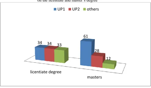
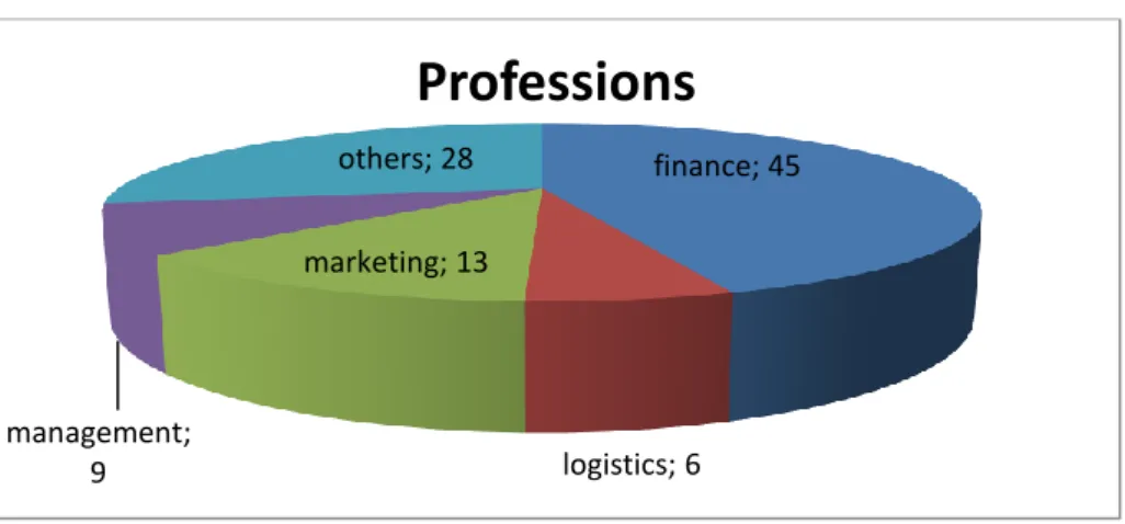
graphic 1 - sample characterization according to faculty frequented on the licentiate and master’s degree ... 45 graphic 2 - sample characterization according to faculty and course frequented on the licentiate degree ... 45 graphic 3 - sample characterization according to faculty and course frequented on the master’s degree ... 46 graphic 4 - sample characterization according to course frequented on the licentiate and master’s degree by the UP1 alumni ... 48 graphic 5 - sample characterization according to work area ... 49 graphic 6 & 7 - sample characterization according to university frequented on the licentiate and master’s degree by the alumni working in finance (graph 6); sample characterization according to course frequented on the licentiate and master’s degree by the alumni working in finance (graph 7) ... 50
0
Cap I – Introduction
1.1 – Framework
In today’s world, any job comes with a list of knowledges that one must have to apply but for almost all of them finance is a part of that list and therefore a critical discipline for the students to know. As a discipline, finance is also a complex and always evolving subject which makes it hard to teach but also critical to nail the basic instruments that compose it, to create a finance base that, if the finance world continues to evolve and change, can provide for the alumni the capacity to cope with this evolution and be able to learn the new instruments easier and quicker. The level of efficiency that this finance base is created is a key factor for each university to study and, therefore, it is the topic of this thesis.
To study it the first step was to define the financial instruments present on this financial base. A lot of different possible books were explored and to create this base, considering that the idea was to approach finance as an all and debate the efficiency of its teachings at a university level, the books read and studied should be the most influential and still actual books on the topic, regarding that all the books combined would explore all the existing financial fields. The two thesis advisors, professor Renato Costa and professor Renato Pereira, advised to read the following books in finance: Brealey and Mayer and Allen; 2016, Copeland and Weston and Shastri, 2013, Damodaran 2014, Carvalho das Neves, 2005. From them some financial instruments were chosen to create the questionnaire that although, as said before, the questionnaire was destined to the ex-students from ISCTE and ISEG, the financial instruments included are not chosen based on what is explored by the finance teaching programs of the two institutions but by their relevance to the financial field as a whole.
In order to simplify and gain some clarity, the teaching efficiency was studied in the contents efficiency rather than the teaching format efficiency, i.e., the questionnaire only focuses on if the alumni know the instrument and not if they know it well or poorly. This took the focus of the teachers and the financial program of each faculty.
The Two faculties were named Public university 1 (“universidade publica 1”) and public university 2 (“universidade publica 2”), or UP1 and UP2 for short. To keep some confidentiality on the subject there will be no information on which university is UP1 or UP2.
1
1.2 – Problems of the investigations
Due to how specific the topic is this thesis has some problems in the investigation process from the start. The ones identified may not be the only ones but are the ones that in some way were dealt with before the investigations started.
The first one is how difficult it is to define what comprehend the financial discipline and the way it was dealt with was already explained, by using different renown financial books and authors.
The second aspect was to define a true base of financial instruments for each financial field and it was dealt in a different way. All the authors had slightly different opinions about the same financial field and it was hard because of it determining a true base of financial instruments for each financial field. The problem was dealt with by selecting an author from the ones read, to base most of the financial fields and the one chosen was Damodaran 2014 due to being the author that dealt with every field and the most known one. This lead to the instruments selected for the questionnaire that are not to be considered fully representative of each financial field. There was a clear solution to this problem and it was to use the finance programs that the faculties had to define each area but doing so could bring some bias towards one of the faculties by choosing more instruments from UP1 or from UP2 to define a financial field. It could also violate the proposition of determining an independent base of instruments that could be applied to any university and be used in any student so for this reason, and the one before, this road was not taken.
The third problem was the sample equal distribution, of students from each university at the masters and licentiate degree level, needed to make the analysis fair. This was a problem because most students either take one of the degrees outside of these two universities or they take one of them at UP1 and the second one at the UP2, or vice versa, making it hard to construct a perfect sample. This problem was managed by selecting one of the two degrees to have a perfect distribution and then focusing on getting the other one as perfect as possible. The degree selected was the licentiate degree and the master’s degree data were always analyzed, knowing this problem.
1.3 – Thesis structure
The investigation process of this thesis relays almost entirely on the questionnaire and so the first step of this document was to define the structure of said questionnaire and from where to
2
take the instruments that compose it. This is present in the literature review as well as all the books used to produce it and the steps and decision behind the definition of each financial field. The second step relates to the methodology used when gathering the sample needed and analyzing it. This helps to have a clear picture of the methods used for the investigation and the assumptions taken to further it.
The third step is divided into two chapters, one that defines the sample characteristics and one that presents the data collected in the form of three tables, that collect the data used for this analysis. In the second chapter it will be presented as well as the data used on each research question study.
The fourth step comprehends the data analysis of this thesis, focusing more on explaining the results obtained and comparing them with the what were the initial expectations. The sample gathered was not perfect and therefore had some influence on the data gathered so in this chapter any misconception that could come from the sample distribution were discussed and defined as such.
Lastly the fifth step was the conclusions taken from this thesis analysis. They were done with the clear idea that this thesis proposition was not to achieve any specific objectives but to define and create a clear image of the teaching efficiency of finance. Some conclusion came as obvious due to how close the results came to the expectations but are not to be considered as final answers to the problems identified.
3
Cap II – Financial instruments and their analysis parameters
This literature review will try and explain the different financial instruments chosen while mentioning the books from where they were taken from. The explanations of every financial instrument will be very simple, in the hopes that any reader can make sense of some complex financial subjects and understand the reasons why we thought they were important enough to be included in the questionnaire. If by reading the explanations you still are confused about the reason some of the instrument are important enough to be included, we advise you to read the books mentioned on the explanation of each financial instrument. All the books are known worldwide and they all try to explain every dimension of finance, going in on each of these dimensions with different depth, and so most if not all of the financial instruments that are included in this questionnaire are present in more than one book. The books mentioned in each instrument are the ones that not only included the instrument on their book but also gave a more complex and complete explanation of what it is used for.
This chapter will be divided in 6 parts where each one will be about a specific aspect of finance and will be about more than one question asked on the questionnaire. There will be an explanation about what is the instrument, were the objective is to explain it in a way that is simple, short and intuitive; and then following this explanation there will be a procedure explanation where, without explaining all the formulas and their mathematical deduction, we will show what they are used for and how to achieve the final value. The order of the explanations will be different from the order of the questionnaire and the parts are: part 1 - risk models; part 2- investment decision rules; part 3 – dividends; part 4 - internal analysis; part 5 – ratios; part 6 - optimal financial mix and part 7 – option
2.1 – Risk models
2.1.1 - CAPM, APM, Multi Factor and Proxy Models
To determine if a new project is good enough to invest in, it´s important to account for all the variables that may affect the success of that investment, in other words, the risk of the project failing. To determine this risk, we must first understand that risk comes in two shapes, firm-specific risk and market risk. If you have all your money in one company, company X, you will be exposed to both types of risk, because you are vulnerable to company X firm-specific risks
4
and the market risks that affects all companies in the market. This is what happens to every owner of a company that has most its money invested in their own company. Despite these types of investors, most aren't like this, you can choose to invest in hundreds of companies and avoid being exposed to a firm's risk of failure and therefore be only exposed to market risk (Ullah et al 2017, Amaya et al. 2015).
This process is called diversification and it cuts down the firm specific risk to almost zero, gathering in the same portfolio more than one firm per market so that if you invest in two companies that compete in the same market, in the case of one of them failing, the other will raise in value, of setting the losses of the first one. However, it does not change market risk because if the market the two companies operates in drops in value you cannot off set this loss directly with a gain elsewhere making it impossible to eliminate market risk through diversification. These types of multiple investments are designated as market portfolios (Olsen 2016).
This market portfolios may reduce the volume of firm specific risk that you are affected by when making investments, but you still must calculate how much market risk affects each investment and to do so the financial instrument used are the market risk measuring models. They use a simple concept which states that in the market there are risk-free assets and risky assets and every investor holds a combination of both. To make an investment in a risky asset worth it the assets must first make a return higher than the return on a risk-free asset. Then you should consider how it will affect the return on the investor existing portfolio, i.e., on the investors existing investments. This concept is called the risk premium, or hurdle rate, because it's the premium return, or rate of return, demanded by an investor to change from a risk-free asset to a risky asset. The risk-free asset return will be calculated using the return on a govern treasury bond of the country the currency is from or, if the govern treasury bond isn't secure enough, by converting the investment currency to a more stable currency and using the return on the treasury bond. being the top traded currency and the most solid global economy, the USA treasury bond is the most used (Brealey et al. 2016).
The way a risky asset is calculated will depend on the model that you are using and is calculated through a variable called Beta. The models vary in what they think impacts market risk and the beta reflects the variation the asset makes in the variable being considered by that model. These returns are all calculated in percentages of the return on the initial investment making it independent of the volume of the initial investment.
5
In this questionnaire, there will be included two of the most known models, the APM and the CAPM, and two lesser known which the multi-factor models and the proxy models are. All the models are entirely dependent on the market portfolio and make some assumptions regarding every investor which are that there is no private information, there is no transaction costs, everyone holds a market portfolio and this market portfolio has every traded asset. With these assumptions, they consider the marginal investor, the stock holder that will be the first to sell, to be someone that matches all these definitions and that has a small quantity of the company. He will react to any bad investment and sell at a lower price than the value of the stock (Damodaran 2014).
The CAPM, or Capital Asset Pricing Model, defines market risk as the risk added by the
investment to the market portfolio and calculates the beta by relating the beta of the investment to the beta of the market portfolio (Fernandez 2015; Copeland et al. 2013; Carvalho das Neves. 2005).
𝐸(𝑅𝑖) = 𝑅𝑓 + 𝛽 ∗ [𝐸(𝑅𝑚) − 𝑅𝑓]
The APM, or Arbitrage Pricing Model, it tries to define what are the factors responsible for the
market risk that are common to every investment. The market risk is the risk exposure the investment made must the factors defined, and it uses multiple betas, each one related to a factor being considered (Davidson 2015; Damodaran. 2014).
𝐸(𝑅) = 𝑅𝑓 + 𝛽1 ∗ [𝐸(𝑅1) − 𝑅𝑓] + (… ) + 𝛽𝑛 ∗ [𝐸(𝑅𝑛) − 𝑅𝑓]
The Multi-factor model, expands on the APM and tries to define the factors responsible for
the market risk using only macro-economic factors, based on the premise that if market risk influences every investment, no matter where you are, then it must come from macroeconomic variables. It calculates market risk by analyzing the risk exposure to the specific asset as to the economic factors and as the APM uses multiple Betas that are al based upon macro-economic factor (Brealey et al. 2016; Lohrmann 2015).
The proxy model is the only one that explore a different method than the previous 3 models.
It uses the historical data on the returns of the previous investments and analyses the factors behind the differences in return from one investment to the other, in a year to year frequency. Uses proxy variables instead of betas and calculates them using a linear regression between the
6
factors responsible for the variances in the return. The market risk is captured in this proxy variables (Carlin 2015, Damodaran 2014).
𝑅𝑡 = 1.77% − 0.11 ∗ ln(𝑀𝑉) + 0.35 ∗ ln (𝐵𝑉 𝑀𝑉)
2.1.2 - Betas
The betas are a statistical variable that correlates the risk in investing in a specific asset with the risk of investing in an asset influenced only by a specific variable. This variable can be the risk of the market portfolio, as used by the CAPM, or a more specific variable such as changes in industrial production, as used in the APM or multi-factor model.
To calculate these betas there are three different methods that will all use the same concept of trying to determine how much does external factor change the earnings of a company from one year to the other and what are those external factors. Then they will try to compute a beta that retains all these factors (Brealey et al. 2016, Damodaran 2014, Carvalho das Neves, 2005). The first one is the Historical beta and it's the most common method used, mostly because it includes the service beta, but also because it is the simplest way of calculating the betas. It relies heavily on a good definition of a market portfolio and the accuracy of the historical data. The process of calculating it is by doing a linear regression between the return on an investment and the return on the market portfolio, the slope of this regression is the beta of your company (Serra 2018, Damodaran 2014).
𝑅𝑗 = 𝑅𝑓 + 𝛽 ∗ (𝑅𝑚 − 𝑅𝑓) ⇔ 𝑅𝑗 = 𝑅𝑓(1 − 𝛽) + 𝛽 ∗ 𝑅𝑚
The Service beta is, as mentioned above, included in the historical beta method because they are calculated using the same method. The process of calculating the beta can be complicated and tedious to do, in which you must consider a lot of different constants, so most companies use external services to obtain their beta and the beta associated with their next investment. They are calculated by private firms that profit from selling their beta calculator software to other firms. The reason they are considered a different classification is because, although all the service betas are calculated with the same base method of linear regression, each firm has a slightly different method of calculating their beta that they don't reveal to the public (Otuteye et al, 2017; Damodaran 2014).
7
The second one is the Fundamental beta which focus on the fundamentals of a company and uses this to then compute the value of the beta. This is based on the premise that the company is not defined by their return history but by the decisions it made on where to investments their money and the overall philosophy it follows. The beta is influenced by three factors: the type of business the firm is in; the degree of operating leverage; and the financial leverage it uses to finance each investment. The first factor considers the pre-existing beta and compares it to the market averages, the second one considers how the firm’s operations are financed and their cost composition; the third one adds the financial structure of the firm to the beta. By combining these three factors we have a beta that can easily be applied to compare your firm to the market, even one that is not publicly traded by using directly the average of the market. It's also more dynamic, changing from one investment to the other on multiple factors at a time, making it more sensitive to different investments on the firm (Brealey et al. 2016; Kwan 2016).
𝑑𝑒𝑔𝑟𝑒𝑒 𝑜𝑓 𝑜𝑝𝑒𝑟𝑎𝑡𝑖𝑛𝑔 𝑙𝑒𝑣𝑒𝑟𝑎𝑔𝑒 = %𝑐ℎ𝑎𝑛𝑔𝑒 𝑖𝑛 𝐸𝐵𝐼𝑇 % 𝑐ℎ𝑎𝑛𝑔𝑒 𝑖𝑛 𝑠𝑎𝑙𝑒𝑠 𝛽𝑢 =𝛽𝑙
[1 + (1 − 𝑡) ∗ (𝐷𝐸)] ⁄
The last one is the Accounting beta that uses accounting earnings instead of traded prices or market values. This method measures the beta again with a linear regression but instead of using market return on investment and return on the market portfolio as the two variables, it uses the changes on accounting earnings, in the firm or in a division of the firm, versus the changes in earnings for the market. Although it is a more intuitive method it has some downfalls, as accounting earnings are vulnerable to the accountant’s allocation of expenses and income, to the non-operating factors; such as depreciation; and to the number of observation used on linear regression, which is substantially less than the other methods, because accounting earnings are only computed, at best, on a quarterly basis and the market value are computed daily (Brealey et al. 2016; Copeland et al. 2013; Damodaran 2014).
2.1.3 - Final considerations
For this part of the questionnaire we have decided to include some method of calculating risk that aren't the most commonly use on the books, the multi-factor model and the proxy model. The most common models are the CAPM and the APM but they have one problem which is
8
they both rely too much on the existence of an effective market portfolio which the proxy model does not rely as much. They also lack the problem of using either only one beta to explain all the risk, the CAPM, or on multiple but unspecified beta to explain the risk, the APM. This last characteristic is also a problem on these two risk models, that is solved by the multi-factor model that tries to also explain the risk in multiple factors, identifying that the use of only one beta can be limited, yet it also tries to give a more specific answer to what betas should be used by using only macro factors.
2.2 - Investment decision rules
Investing in a project is not only about considering the risk involved and the return around it, it's also about the earnings and cash flow that come with the new project. By relating the hurdle rate and the earnings we can directly determine if a project will bring value to the company or not but there is a problem, they can't be directly related. This is because the hurdle rate returns a percental value and the earnings and cash flows return a value in dollars, so we must use a financial instrument, explained in this part 2, that will serve as a tool to indirectly relate these two variables and allow us to use this method to accept or decline a project, based on the value it will bring to the company (Brealey et al. 2016).
2.2.1 - Bases for investment decision rules
There are 3 different types of instruments that can be used to make investment decisions using the earnings, they are the accounting earnings based decision, the cash flow based decision and the incremental cash flows based decision. Every company has their own rules to make investment decisions and they normally use more than one of this investment decision rule but to assure that they are useful and well defined it should have a balance between allowing the influence of the manager to help the decision and be able to analyse every investment consistently, no matter the volume of earnings it has. They also have to prioritize investments that bring value to the company and must work to every different kind of investment. In a company that uses more than one investment rule, one of them is defined as a primary rule, so that it can work as a tie breaker. Here follow the three types of investment decision rules:
9
The accounting income-based decision rules is defined by drawing the earnings data from the accounting statements and accounting measures of income. This method uses the accounting values for earnings and divides them with the average book value of the investment in the project. It can deliver two different values depending on the value s you consider, if you use the total accounting earnings and the book value of the investment, then it is called the return on capital; if it uses only the equity invested in the project and the net income, also known as the income to equity investors, it is called return on equity. These two financial instruments of return give a percentage value of the earnings gained on the investment and therefore can be compared to the appropriate hurdle rate, return on capital to the cost of capital, and the return on equity to the cost of equity. If the return is higher than the hurdle rate, then the investment
will bring value to the company and should be accepted (Rohrbeck et al. 2018, Copeland et al.
2013, Damodaran 2014).
In the questionnaire, these types of investments decision rules will not appear in this part because they will be used in one of the methods to calculate the optimal financial mix, to assure that the questionnaire isn't at any point repetitive and because these two instruments aren't solely recognized as an investment decision rule but also as part of different financial processes. The cash flow-based decision rules result of the inefficiency of the accounting earnings to always being right. Sometimes the cash flows and accounting earnings deviate and when these cases happen the use of the cash flows value is preferred therefore there is an investment decision rule that uses cash flows instead. There are two perspectives on this instrument and the first one is not a different instrument but rather the use of the return on capital and equity with cash flows and cash returns rather than with accounting values. The other perspective involves a new method but again not necessarily a different financial instrument. It's called the payback and it is the amount of time the project takes to return the initial investment, also known as the payback period of the project, upon which the project becomes a source of profit. The payback is a way to quickly and intuitively determine if a project has a low risk by using the payback period as a measuring system. If the project has a low payback period then it's reasonable to assume it has a low risk, since a significant portion of the risk in an investment is related to the possibility of losing the initial investment (Adamczyk et al 2017, Brealey et al. 2016, Campos et al 2016, Copeland et al. 2013).
For this part of the questionnaire there are also no questions about these types of investment decision rules. The decision was not made based on the usefulness or capacity to work on any
10
case of both the instruments because both are considered, specially the payback, by all the authors in the literature review, as being exceptional and used by most if not all the investors. The decision was made in a more practical perspective of how to include them in the questionnaire. The first one is an adaptation of the return on capital and equity previously discussed on the accounting based decision rules and the second is not a clear financial instrument and cannot be used as an individual investment decision tool, so the decision was to not include any of the two-cash flow-based decision rules on the questionnaire (Damodaran 2014).
The discounted cash flow-based rules goes one step forward than the previous rule and substitutes the accounting income with discounted cash-flows, considering here the time value of money. The two instruments in this investment rule are the net present value and the internal rate of return and are considering competitors, among investors, for the most used investment decision rules, and the reason is obvious, they are the only ones that use discounted cash-flows. The discounted cash flows come as a necessity to consider the time value of money, very easy concept to understand that states that a dollar today is more valuable today that it will be tomorrow. This comes by the fact that if you have one dollar today instead of tomorrow you can invest it at the tax rate and tomorrow they will value more than the original dollar. Applying this concept to an investment with a more than one year life span, using this idea to look ahead, you can conclude that one dollar tomorrow will value less than one dollar today so, when adding up all the value this investment will bring to the company today, you can't add them all without considering this. Here comes the discount rate that will reflect just that and will represent the actual value of all the cash flows on that project. This rate is most times considered to be the cost of capital or the cost of equity (Brealey et al. 2016; Declerck 2016; Damodaran 2014; Copeland et al. 2013).
2.2.2 - The two instruments for discounted cash-flow decision rules
The net present value, also known as NPV, is calculated by adding up all the cash flows, positive or negative, that a project will have in each year including the initial investment considered in year zero. In this process, it will use a discount rate depending of what cash flows it is considering. This returns a dollar value that reflects the value the project will return to the firm at the end of its lifetime.
11
This financial instrument has two perspectives to consider. The equity investors perspective that will be calculated using the cash flows to equity, discounting them using the cost of equity and netting out the initial equity investment and the perspective of all the investors that will be calculated with the use of the cash flows to the firm, discounting them with the cost of capital and considering the total initial investment (Willigers et al 2017; Brealey et al. 2016).
The internal rate of return, also known as IRR, is the value of the discount rate that will bring the NPV down to zero. In a more conceptual way it is a perceptual measure of the return you are getting in an investment, towards the discounted cash flows. It is a simple way of considering the NPV and throw it reaching a percentage value for the return which makes it more useful and easy to then compare to the hurdle rate defined. If his percentage value will be higher than the hurdle rate then the project should be accepted, if it is lower than it then the project should be denied.
Again, it can be used with two perspectives, the equity investors and all the investors. The first one demands the use of only cash flows to equity investors to calculate the NPV and then the comparison with the cost of equity. The second one uses the NPV of all the cash flows and
compares it with the cost of capital (Gharari et al 2015;Damodaran 2014).
𝑁𝑃𝑉 = ∑ 𝐶𝑡 (1 + 𝑟)^𝑡 𝑡 𝑡−1 − 𝐶0 𝐼𝑅𝑅 𝐼𝑠 𝑤ℎ𝑒𝑛 𝑁𝑃𝑉 = 0 ⇔ ∑ 𝐶𝑡 (1 + 𝐼𝑅𝑅)𝑡 𝑡 𝑡−1 − 𝐶0 = 0 2.3 – Dividends
In this chapter, we go through the two aspects related to the dividend decision, the first one is the process of deciding what philosophy the company will follow of how much to pay in dividends and how to determine that value, and the second one is how does the market react to the amount of dividends paid by a company and the instruments used to measure it (Eldomiaty et al 2015)
12
2.3.1 - Company philosophy about dividends
Dividends are an integral part of the business of every firm that they, once a year, must think about and decide whether or not to distribute them and how much they should distribute. In the case of publicly traded firms this is a bigger problem related to how much money to distribute to get a respectful amount per stockholders, in contrast with privately owned firms where it is simpler but also something to be considered. In their case instead of having multiple stockholders to distribute the dividends you only have a few, so the amount per stockholder will be larger, but because it is harder to a private firm to get financial aid they have to consider a larger portion of the earnings to reinvest in the firm.
The reaction of the market, or the changes on the stock price due to the amount of dividends paid will mostly happen on two dates set by the board of directors; first is the dividend declaration date, when the board of directors declares how much money they will pay on dividends and if they will decrease, increase or maintain the value of dividends paid in the previous year. This is the date on which markets will react to these changes in the dividends paid so if they due occurs then the market value of the firm's stock will also change accordingly in that date. Then follows the ex-dividend date that establishes the date after which, if someone buys the stock, they will no longer receive dividends. At this point the price of the stock will fall to reflect the value received in dividends that will no longer happen (Ivanovski et al 2015; Damodaran 2014; Copeland et al. 2013).
In the dividend decision process, there are three different schools of thought, the one that states that dividends are irrelevant, the one that defends that dividends are bad to the stockholder and the one that says that dividends are good to the stockholders.
The "dividends are irrelevant" follows the principle that there are no tax disadvantages for the stockholders from receiving dividends and that firms have no additional issuance costs when raising funds in capital markets for a new investment, so there is no benefit from holding on to earnings to make new investments. Adding to this, this theory also relays on the premise that, the operating cash flows don't change with the variation of the dividends paid and that the managers will not use the free cash flows to pursue their own interests such as investing in bad projects to hurt the firm but favour them (Brealey et al. 2016; Copeland et al. 2013).
Although strange this is common when the managers have a lot of power over the board of directors and therefore don't have to follow the stockholders needs opting to use the firm to achieve their own goals that may or may not lead to value maximization of the firm. This was
13
a big problem in the 90's that got resolved with creation of new laws that protect the stockholders and create more effective board of directors, such as having outside of the firm members on the board of directors (Damodaran 2014).
The dividend policy will also be irrelevant, meaning that the amount of dividend you pay will not be related to the earnings in that year and will not directly affect the value of the equity. This however will not change the fall on stock price value after the ex-dividend date because at that point in time the amount of dividends paid is not responsible for the fall of the stock price, there is no amount of dividends paid that can cover the fact that after that date no dividends will be received so, if you buy the stock, the value of the stock must go down to reflect that loss
(Brealey et al. 2016; Varma et al 2016; Copeland et al. 2013).
The second school of thought, "dividends are bad", argues that receiving dividends brings a tax disadvantage to the stockholders. To understand this, it's important to first explain what happens if the firm does not give dividends. The extra income stay's in the company as free cash flow and can either be used to repurchase stock, make new investments that add value to the firm or just to accumulate the money for any eventuality. All these activities have one thing in common, they all raise the initial value of the firm's equity, that then raises the overall value of the firm, consequentially increasing the stock price value. This increase on the stock price is considered to the stockholder as a capital gain. If the company decides to distribute dividends instead of retaining them or applying them the stock value will remain the same and the stockholder receives an ordinary income.
Here lays the problem with the tax disadvantage, because the ordinary income has, in some countries, a different, much higher tax rate than the capital gain has, which leads to this dividend school of thought conclusion that paying a high dividend will reduce the firm's stock price, because stockholders will value this stocks at a lower price than other stocks that pay less dividends due to the advantage of receiving their money through capital gains instead of
dividends (Angulo-Ruiz et al 2018;Brealey et al. 2016; Damodaran 2014).
This school of thought only works on one assumption, that the marginal investor, i.e., the stockholder most vulnerable to changes making him the first to sell the firm's stock if something does change, is an individual investor and not a pension funds and institutional investors. These two types of investors don't share the same tax problem as the individual investor because they are tax-exempt, so firms with stockholders predominantly from pension funds or institutional
14
investors may not create a tax disadvantage problem to their investors, and therefore are ok with paying a high dividend (Damodaran 2014; Copeland et al. 2013).
With this tax disadvantage comes also an investment opportunity. After the ex-dividend date, the fall on the value of the stock happens to reflect the preference for dividends. With this theory of a harder taxation of the ordinary income, the fall should be considerably smaller than the amount of dividends paid to accommodate the tax preferences of the marginal investor. Considering this premise there is a possibility for an investor to trade around the ex-dividend day and make excess returns, as long as its tax benefits are higher than the ones of the marginal investor. This action is called dividend capture or dividend arbitrage and is a very risky process and only works on stocks with high dividend yield due to the transaction costs associated with it (Damodaran 2014, Copeland et al. 2013).
The third and last theory is the "dividends are good" which says that notwithstanding the existence of a tax disadvantage, firms still pay dividends so there must be some good reasons to do it and here we will first discuss two ideas that aren't entirely true and then present two real advantages of using this dividend school of thought.
The first reason is related to the stockholder perspective of capital gains, that see it as an uncertain source of cash when compared to the immediate cash return from the dividends. They prefer the later form of income, more specifically, they prefer receiving dividends now and not capital gain in some point in the future, ignoring the tax disadvantage associated with it (Brealey et al. 2016, Damodaran 2014).
This is a false argument for two reasons, The first one is because, as it has been discussed in the "dividends are irrelevant" portion, the reaction of the stock price to the payments of dividends occurs at the same time as dividends are paid to the investors, decreasing the value of stock slightly less than the value of dividends being paid, so it is reasonable to believe that the capital gains, resulting from paying less dividends, will happen in the present and not in the future. The second one is, if a company decides to pay more dividends but doesn't change their investment policy, to invest in new projects it will have to finance them by issuing more stock which will cause a decrease in the stock price and lead to the stockholder that prefers a higher dividend to lose more money in price appreciation, than they will in dividend gain (Damodaran 2014).
15
The second reason to consider in the dividends are good school of thought is the temporary excess cash available at the end of the semester. Companies tend to fall to the temptation of using this extra income to pay an extra dividend to their stockholders and stockholders prefer them to do so to avoid managers having excess cash available. By doing so the expectation for the next year will be to receive a high dividend again. If this cash excess is a temporary phenomenon, then the company must issue more stock to finance the high dividend it started to pay which again does not bring any advantage to the stockholders (Damodaran 2014).
There is obviously some validation to this dividend policy, that brings some valid arguments with it and the first one has already been referred previously which is investors that have low taxes or none, like to receive dividends because, in contrary to an individual investor, after taxes what they get from dividends is higher than what they would get in capital gain. There are also investors that have some valid reasons to prefer receiving dividends, such as the need of a regular cash flow from the dividends to make their own investments or because they don't have an easy way of liquidising their capital gains. Companies with an history of paying high dividends have mostly investors with these characteristics and because of that paying dividends will be a good thing to their stockholders. Companies may also use dividends to reach their optimal financial mix, to reduce the amount of free cash flow available to the incompetent managers and therefore control the conflicts between managers and stockholders; and to use it as a way of signalling the markets that the company will have some positive future years (Brealey et al. 2016, Damodaran 2014, Copeland et al. 2013).
2.3.2 - Dividends based instruments to study the market
This last point is the focus of the second part of our questionnaire surrounding dividends. The markets use that information to understand the future of the company and react to these changes in the dividends policy. A company only raises dividends if it is confident that they will be able to pay them not only in the present year but also in the future with cash flows and not with contracting debt and knowing of this relation between dividends and cash flows, the markets will react positively to the raise of dividends, and negatively if the dividends fall (Brealey et al. 2016, Copeland et al. 2013).
To analyse these changes and then compare them to other firms there are two important ratios used by most analysts, the dividend yield and the dividend payout ratio.
16
The dividend yield is the ratio between the amount of dividends paid and the stock price and, when added the price appreciation, it is used to calculate the return on the stock. It can also be used as a measure of risk and as an investment screen, meaning, as a direct way to tell if a stock will have a good return or not (Brealey et al. 2016, Damodaran 2014, Copeland et al. 2013)
𝑑𝑖𝑣𝑖𝑑𝑒𝑛𝑑 𝑦𝑒𝑙𝑑 = annual dividends per share 𝑝𝑟𝑖𝑐𝑒 𝑝𝑒𝑟 𝑠ℎ𝑎𝑟𝑒
The other ratio is the dividend payout ratio which will relate the dividends to the earnings of the firm and can be used in valuation of a firm, in calculating the retention rate that gives an
insight in future growth of earnings and in determining the current life cycle of a firm(Brealey
et al. 2016) and (Copeland et al. 2013).
𝑑𝑖𝑣𝑖𝑑𝑒𝑛𝑑 𝑝𝑎𝑦𝑜𝑢𝑡 𝑟𝑎𝑡𝑖𝑜 =𝑑𝑖𝑣𝑖𝑑𝑒𝑛𝑑𝑠 𝑝𝑒𝑟 𝑐𝑜𝑚𝑚𝑜𝑛 𝑠ℎ𝑎𝑟𝑒 𝑒𝑎𝑟𝑛𝑖𝑛𝑔𝑠 𝑝𝑒𝑟 𝑠ℎ𝑎𝑟𝑒
2.3.3 - Final considerations
One cannot apply these ratios to analyse a firm’s future without understanding how the relation between dividends and earnings work. They are positively related, this means that if earnings rise or fall dividends will also rise or fall but they will do this with a certain lag, changing sometime after the changes in earnings has occur. The dividends are also sticky, which means that once they are following a rising or falling trend, they will hardly change in the future, because managers are reluctant to change the amount of dividends they pay, afraid of the possible negative reaction markets have when the dividends change and the expectations they create with that change. As said before the dividends will raise with the earnings but this fear leads managers to be more inclined to slightly increasing the dividends even if the earnings are decreasing, which means that dividends will take more time than the earnings to adjust to the real value they should be, leading sometimes to misleading information taken from the dividend payout ratio or the dividend yield. These two instruments are two key methods of taking information's from the markets and therefore they are included in the questionnaire in this part as a way of acknowledging that dividends are indeed a quick way of understanding a company's future cash flows and life cycles (Damodaran 2014).
17
2.4 - Internal analysis
Until this point all the investments were long term and therefore discussed in the point of long term actions and financing, but there are also short-term needs from every project, especially in financing the business cycle operations of a project. To understand this concept and to apply it we must first understand that these are also investments but smaller ones and considered internal investments, made to cover the operational needs of a company in the short-term for all their current projects. This value although part of the short-term interests of a firm, can influence and condition the long-term investments by taking up a big part of the financial leverage a firm has, that could have been used to finance long-term projects. There are a lot of financial instruments that can be used to do this analysis but there are 3 key ones that we decided to include in this questionnaire: the working capital needs, the financial leverage and the operational leverage; and they are explained in the following chapters (Hofmann et al 2016; Damodaran 2014; Carvalho das Neves, 2005; Capizzi 2005).
2.4.1 - Noncash working capital
In the mathematical formula, the working capital is the difference between the current assets and the current liabilities, which in practice reflects the operational needs of the company in each business cycle. The current assets are considered to be all the assets that are in the form of cash or will be converted to cash in the short term, that is in less one year, and generally include the inventory, cash, marketable securities and accounts receivable. The current liabilities are all the company's debts and obligations in the short-term and they include the short-term debt,
accrued liabilities and accounts payable (Brealey et al. 2016; Hofmann et al 2016;Carvalho das
Neves, 2005).
because in the duration of the investment it will be necessary money to produce the product or service, either with investments in inventory or with investments in qualified people because of this, when making a new investment, it's necessary to consider the working capital. This will tie up some additional cash flows to the initial investment in the project because these working capital investments are cyclical, so they will happen every year, and if you don't consider the working capital of a new project you may end up with no financial capacity in the short term to run said project.
18
After defining what is the working capital we can now understand that in every business cycle the amount of working capital may change depending on a variety of factor, such as the number of units a company projects to sell, how much the account receivables and payables are expected to grow or how much of these changes will be paid with short term debt, etc. As you can see there are a lot of variables that come to play so we can consider that the working capital is driven by demand and it is necessary to estimate the working capital needs every year. To do it we must relate it with another financial variable and consider it as a percentage of that variable. The most common variables used to calculate the working capital as a percentage of, are the revenues, the operating expenses or to calculate it per the number of units sold. As in every step of a new investment, the estimates for the working capital becomes more accurate if the firm has done similar projects in the past (Damodaran 2014).
This method of estimating the working capital needs is only an average number, that does not represent directly the real expenses of working capital. As said in the beginning of this chapter there is a formula to calculate the working capital using the data available of the previous year. It uses this data to determine how much working capital expenses the firm had in that year and then estimates the next years working capital needs. This is the formula present in the questionnaire because it is the most common method in all the books and the most accurate one
(Brealey et al. 2016; Lourenço et al 2009;Carvalho das Neves, 2005).
𝑤𝑜𝑟𝑘𝑖𝑛𝑔 𝑐𝑎𝑝𝑖𝑡𝑎𝑙 = 𝑐𝑢𝑟𝑟𝑒𝑛𝑡 𝑎𝑠𝑠𝑒𝑡𝑠 − 𝑐𝑢𝑟𝑟𝑒𝑛𝑡 𝑙𝑖𝑎𝑏𝑖𝑙𝑖𝑡𝑖𝑒𝑠
𝑁𝐹𝑀 = 𝑐𝑖𝑙𝑖𝑐𝑎𝑙 𝑛𝑒𝑒𝑑𝑠 − 𝑐𝑖𝑐𝑙𝑖𝑐𝑎𝑙 𝑟𝑒𝑠𝑜𝑢𝑟𝑐𝑒𝑠
2.4.2 - Degree of Operational and Financial leverage
When analysing a firm stability, it's important to analyse the operational and financial volatility. To do it we have to look for the income statements of the previous years to see how much is the variation in operational costs or how much debt dependant is a company to then determine the component of risk associated with these two variables.
The operational costs come in two types, the fixed cost, that will remain the same if the company increases the volume of production, and the variable cost, that vary with the volume of product output, rising if the production increases and falling if it decreases. A company with a higher percentage of fixed costs will have a high operational leverage. This is a situation to be avoid
19
by a company with volatile sales because they will have a more than proportional effect on operational profits, making a bigger impact if sales drop, but to be embraced by a company if the sales have a tendency of rising because in this case having a bigger percentage of fixed costs will provide a more than proportional rise in operational profits (Brealey et al. 2016;
Damodaran 2014; JORDAN et al 2008).
The financial leverage is an important tool when analysing the financial structure of a company so that you can ascertain their ability to pay the financial obligation towards debt owner in the short or long term. Even a company with a perfectly balanced financial structure may not earn enough from sales to pay their short-term commitments, so to determine how vulnerable a firm is to the use of debt to finance itself, analysts use the financial leverage that will relate the operational profits to the current earnings. These financial instruments also allow to determine if using debt will have a positive or negative influence in the profitability of a firm (Damodaran 2014; Vieira et al 2006; Carvalho das Neves, 2005).
To understand how vulnerable a firm is to changes in operational and financial leverage we can use the degree of operational and financial leverage that will deliver a value independent of the dimension of a specific company and can then be used to compare with the companies in the same sector and determine if there should or not be an adjustment to the operational costs or the financial structure. We will ask in this questionnaire about the degrees of financial and operational leverage due to their ability of either use it to understand your own vulnerability or
to compare yourself to the markets (Devashish 2017;Damodaran 2014; Carvalho das Neves,
2005). 𝑑𝑒𝑔𝑟𝑒𝑒 𝑜𝑓 𝑜𝑝𝑒𝑟𝑎𝑡𝑖𝑛𝑔 𝑙𝑒𝑣𝑒𝑟𝑎𝑔𝑒 = %𝑐ℎ𝑎𝑛𝑔𝑒𝑠 𝑖𝑛 𝐸𝐵𝐼𝑇 %𝑐ℎ𝑎𝑛𝑔𝑒𝑠 𝑖𝑛 𝑠𝑎𝑙𝑒𝑠 𝐷𝑒𝑔𝑟𝑒𝑒 𝑜𝑓 𝑓𝑖𝑛𝑎𝑛𝑐𝑖𝑎𝑙 𝑙𝑒𝑣𝑒𝑟𝑎𝑔𝑒 = 𝐸𝐵𝐼𝑇 𝐸𝐵𝐼𝑇 − 𝑖𝑛𝑡𝑒𝑟𝑒𝑠𝑡 𝑒𝑥𝑝𝑒𝑛𝑠𝑒 2.4.3 - Final considerations
These last two instruments are repeated in the questionnaire and represent the only exception to this rule. The exception happens because although the use of these instruments is also present in the fundamental beta and represent almost the same thing as in this part, it's greater use is to make internal analysis of a company, which is the previous part we discussed. There aren't
20
really any other instruments that can do this type of internal analysis that are represented at the same time in more than one book, as the degree of operational and financial leverage are, so to make a section dedicated to the study of internal analysis instruments we had to include them (Graham 2017).
2.5 – Ratios
Ratios are the most used technique by financial analysts to relate different financial-economic variables that otherwise would have no reaction. They are used to synthesize the abundant amount of financial data available and try and make some use of it. They are arranged or constructed to give an inside view of a company to then compare it to other similar companies, to give a quick and easy way to relate two variables that originally would not be related and to help managers make strategic decisions. In a world where speed is of the essence, having a quick way of processing the constant renewing of information is a key factor between failure or success and because of their importance the questionnaire has a dedicate part to the most commonly used ratios on the industry and the ones that were more common in (Brealey et al. 2016, Damodaran 2014, Copeland et al. 2013, Carvalho das Neves, 2005).
To facilitate their recognition and to provide a cleaner look to the questionnaire the ratios are divided in five categories, Liquidity, Financial, Profitability, Functional and Market ratios
2.5.1 - Liquidity ratios
liquidity ratios are used to evaluate the capacity a firm has to pay its own debt with the financial
assets it has in the short-term. These ratios are used mostly by banks when they are coinciding debt to other firms and they are calculated using fiscal units, such as money, time, and workers. They are considered as a marginal security measured by the banks to know how much they will lose if the company they are borrowing money goes bankrupt, ascertaining how much they can take out of them in that situation. The ratios analysed in this part of the questionnaire are "general liquidity", that is used to determine if a company is well balanced or not, and "immediate liquidity", that serves as a tool to know the capacity a firm has to pay their debt with all the available assets (Ismail 2016).
21 𝐺𝑒𝑛𝑒𝑟𝑎𝑙 𝑙𝑖𝑞𝑢𝑖𝑑𝑖𝑡𝑦 = 𝑐𝑢𝑟𝑟𝑒𝑛𝑡 𝑎𝑠𝑠𝑒𝑡𝑠 𝑐𝑢𝑟𝑟𝑒𝑛𝑡 𝑙𝑖𝑎𝑏𝑖𝑙𝑖𝑡𝑦 𝐼𝑚𝑚𝑒𝑑𝑖𝑎𝑡𝑒 𝐿𝑖𝑞𝑢𝑖𝑑𝑖𝑡𝑦 = 𝑏𝑎𝑛𝑘 𝑑𝑒𝑝𝑜𝑠𝑖𝑡𝑠 + 𝑐𝑎𝑠ℎ𝑓𝑙𝑜𝑤 + 𝑛𝑒𝑔𝑜𝑡𝑖𝑎𝑏𝑙𝑒 𝑡𝑖𝑡𝑙𝑒𝑠 𝑐𝑢𝑟𝑟𝑒𝑛𝑡 𝑙𝑖𝑎𝑏𝑖𝑙𝑖𝑡𝑦 2.5.2 – Financial ratios
Financial and operational leverage ratios are the basis of ascertaining the risk of bankruptcy
of a company and determining how much adding more debt to that company will affect said risk. They analyse the operational financial needs of the firm's business cycle and how much of it is already financed by debt, then consider how much of that debt is long term or short term. Finally, these ratios also give a look of the percentage of the current debt that is covered by the cash flows directly from sales or the main source of money of that company. The ratios analysed
in this part of the questionnaire are the " indebtedness”, that ascertains to what extent the
company uses debt to finance itself, the "debt to equity", that does the same thing, the “financial costs coverage", measures the capacity the operational income must pay the financial burdens of the company, and the "results variability" is used to determine if there is risk involved in the firm’s operations. (Mrša et all 2016).
𝑟𝑒𝑠𝑢𝑙𝑡𝑠 𝑣𝑎𝑟𝑖𝑎𝑏𝑖𝑙𝑖𝑡𝑦 = 𝑅𝑂𝑡− 𝑅𝑂𝑡−1 𝑅𝑂 𝑎𝑣𝑒𝑟𝑎𝑔𝑒 𝑓𝑖𝑛𝑎𝑛𝑐𝑖𝑎𝑙 𝑐𝑜𝑠𝑡𝑠 𝑐𝑜𝑣𝑒𝑟𝑎𝑔𝑒 = 𝑜𝑝𝑒𝑟𝑎𝑡𝑖𝑜𝑛𝑎𝑙 𝑟𝑒𝑠𝑢𝑙𝑡𝑠 𝑒𝑛𝑐𝑎𝑟𝑔𝑜𝑠 𝑓𝑖𝑛𝑎𝑛𝑐𝑒𝑖𝑟𝑜𝑠 𝑑𝑒𝑏𝑡 𝑡𝑜 𝑒𝑞𝑢𝑖𝑡𝑦 𝑟𝑎𝑡𝑖𝑜 =𝑒𝑞𝑢𝑖𝑡𝑦 𝑑𝑒𝑏𝑡 𝑖𝑛𝑑𝑒𝑏𝑡𝑒𝑑𝑛𝑒𝑠𝑠 = 𝑏𝑜𝑟𝑟𝑜𝑤𝑒𝑑 𝑐𝑎𝑝𝑖𝑡𝑎𝑙 𝑡𝑜𝑡𝑎𝑙 𝑐𝑎𝑝𝑖𝑡𝑎𝑙 2.5.3 - Profitability ratios
Profitability ratios are as the name says, indicators of how profitability is a company. They
measure this by relating the financial earnings to another capital variable, for example sales. This can also be calculated to be delivering different amounts and return profitability measured per days it takes for a company to be profitable in a business cycle, to the percentage of volume
22
of sales, etc. so that investors can view profitability from different perspectives. It allows the stockholder and the manager to conclude if the profitability of the equity invested is at the level of all the competition, taking into consideration that it is also dependent of the financing policy of the company. Investors overall consider these types of ratio the most impartial indicator to compare one firm to the other. The ratios analysed in this part of the questionnaire are the "sales operation profitability", which computes how much impact sales had in the operational results, the "own capitals profitability", which is used to see how efficient are the investments made with the equity and considers the financial policy of the company, the "assets profitability" and "invested capital profitability", that will do the same as the last ratio but related to the efficiency of the assets and all of the invested capital, respectfully, and therefore will not consider the financial policy of the company (Jubaedah et all 2016).
𝑠𝑎𝑙𝑒𝑠 𝑜𝑝𝑒𝑟𝑎𝑡𝑖𝑜𝑛 𝑝𝑟𝑜𝑓𝑖𝑡𝑎𝑏𝑖𝑙𝑖𝑡𝑦 = 𝑜𝑝𝑒𝑟𝑎𝑡𝑖𝑜𝑛𝑎𝑙 𝑟𝑒𝑠𝑢𝑙𝑡𝑠 𝑏𝑢𝑠𝑖𝑛𝑒𝑠𝑠 𝑣𝑜𝑙𝑢𝑚𝑒 𝑜𝑤𝑛 𝑐𝑎𝑝𝑖𝑡𝑎𝑙𝑠 𝑝𝑟𝑜𝑓𝑖𝑡𝑎𝑏𝑖𝑙𝑖𝑡𝑦 = 𝑛𝑒𝑡 𝑟𝑒𝑠𝑢𝑙𝑡𝑠 𝑜𝑤𝑛 𝑐𝑎𝑝𝑖𝑡𝑎𝑙𝑠 𝑎𝑠𝑠𝑒𝑡𝑠 𝑝𝑟𝑜𝑓𝑖𝑡𝑎𝑏𝑖𝑙𝑖𝑡𝑦 =𝑜𝑝𝑒𝑟𝑎𝑡𝑖𝑜𝑛𝑎𝑙 𝑟𝑒𝑠𝑢𝑙𝑡𝑠 𝑎𝑠𝑠𝑒𝑡 𝑖𝑛𝑣𝑒𝑠𝑡𝑒𝑑 𝑐𝑎𝑝𝑖𝑡𝑎𝑙 𝑝𝑟𝑜𝑓𝑖𝑡𝑎𝑏𝑖𝑙𝑖𝑡𝑦 = 𝑜𝑝𝑒𝑟𝑎𝑡𝑖𝑜𝑛𝑎𝑙 𝑟𝑒𝑠𝑢𝑙𝑡𝑠 𝑖𝑛𝑣𝑒𝑠𝑡𝑒𝑑 𝑐𝑎𝑝𝑖𝑡𝑎𝑙 2.5.4 - Functional ratios
Functional ratios serve to analyse how efficient are the decisions made by the firm and are
usually calculated in terms of product rotation or days of operation. These ratios are specific to each sector because any business sector work in different ways and have different standards for operation, which is fundamental to consider in these types of ratios and therefore they should only be used to compare firms in the same business sector. They can be used to detect how efficient is the use of your assets and to understand if the firm is at maximum capacity, therefore at their own limit or if at the minimum capacity, underutilizing their assets. With these types of ratios, we can also use them to understand how well a firm rotates their stock to understand how quickly a firm receives the money from their sales or business activities. The ratios analysed in this part of the questionnaire are the "invested capital rotation", measures the degree of the assets usage, the "merchandise average storage time", is used to determine the same thing