Adaptive complex system modeling for realistic modern ground warfare simulation analysis based on evolutionary multi-objective meta-heuristic techniques

(1)

MSc Thesis in

Computer Science - Mobile Computing

Adaptive complex system modeling for realistic

modern ground warfare simulation analysis based

on evolutionary multi-objective meta-heuristic

techniques

Diogo Alexandre Breites de Campos Proença

MSc Thesis directed by Professor Silvio Priem Mendes of the School of Technology and Management, Polytechnic Institute of Leiria and co-directed by Juan António

Gomez-Pulido of the University of Extremadura, Spain.

(2)

(3)

II

(4)

III

(5)

IV

Abstract

The battlefield is a harsh and inhuman environment, where deaths and destruction take lead role. Through many millennia there was blood shed all over the world, people who many time died in a battle that sometimes they didn‘t even care about.

Today, the battle field is very different, machines take most damage and there are less casualties, this is because of the advancements made in the fields of aeronautics, weaponry, nautical, vehicles, armor, and psychology.

Also there is another important party that throughout the last decades made a special and decisive advantage to the side which is more advanced in this field, it is intelligence and simulation. Intelligence today gives enormous advantage to one country as you ―see and feel‖ the battlefield hundreds or thousands kilometers away. Then, with the data provided by intelligence, countries can simulate the battle in order to deploy the most efficient units into battle.

In this thesis we propose a warfare simulator analysis tool using a multi-objective approach and artificial intelligence. Further on, the 1991 Gulf war scenario is used to simulate and the results are presented and analyzed.

The approach used in this thesis is difficult to be used in games due to its processing complexity and computing demands.

Keywords: Meta-heuristic, Warfare simulator, Multi-objective optimization, Artificial intelligence, Evolutionary algorithms.

(6)

V

(7)

VI

Resumo

O campo de batalha é um meio adverso e inumano, onde a morte de seres humanos e a destruição têm o papel principal. Desde há muito tempo que sangue é derramado por todas as partes do globo, e muitos desses seres humanos morrem numa guerra que não é sua e pela qual não têm o mínimo apreço.

Atualmente, o campo de batalha é muito diferente, as máquinas é que sofrem o maior dano e há menos mortes. Isto deve-se aos avanços feitos nas áreas da aeronáutica, do armamento, da náutica, dos veículos terrestres, da proteção e da psicologia.

Nas últimas décadas, a informação secreta e as simulações, também tem tido um papel preponderante para as nações mais desenvolvidas. As informações secretas do campo de batalha trazem uma grande vantagem para as nações uma vez que podem ―sentir‖ o campo de batalha a centenas ou milhares de quilómetros de distância. Depois, com a informação recolhida pelos serviços secretos, os corpos militares podem simular o campo de batalha, para que deste modo possam mobilizar as unidades de combate mais eficientes para a batalha em questão.

Nesta dissertação é proposto um simulador de guerra e uma ferramenta de análise utilizando métodos de otimização multi-objectivo e inteligência artificial. A batalha da guerra do golfo de 1991 é utilizada para simular e os resultados são posteriormente apresentados e analisados.

Os métodos utilizados nesta dissertação dificilmente poderão ser utilizados em jogos devido à sua complexidade de processamento e requisitos de computacionais.

Palavras-chave: Meta heurística, Simulador de combate, Otimização Multi-objectivo, Inteligência artificial, Algoritmos evolucionários.

(8)

VII

(9)

VIII

List of figures

Fig. 1. US Deaths in Vietnam and Iraq [37] ... 2

Fig. 2. Terrain representations in highly aggregated constructive simulations [38]. ... 7

Fig. 3. Units case example ... 16

Fig. 4. The general scheme of an Evolutionary Algorithm as a flow-chart [46]. ... 23

Fig. 5. Typical progress of an EA illustrated in terms of population distribution [47]. ... 32

Fig. 6. Typical progress of an EA illustrated in terms of development of the best fitness (objective function to be maximized) value within population in time [47]. ... 33

Fig. 7. Illustrating why heuristic initialization might not be worth. Level a show the best fitness in a randomly initialized population, level belongs to heuristic initialization [47]. ... 34

Fig. 8. Illustrating why long runs might not be worth. X shows the progress in terms of fitness increase in the first half of the run, Y belongs to the second half [47]. ... 34

Fig. 9. 1980's view on EA performance after Goldberg [58][47]. ... 35

Fig. 10. Illustration of Wright's adaptive landscape with two traits [47]. ... 37

Fig. 11. KMeans working example [62]... 46

Fig. 12. KMeans working example 2 [62]... 47

Fig. 13. MOEGWAO static model ... 49

Fig. 14. MOEGWAO Meta-heuristic logic overview ... 50

Fig. 15. Example of combat CRT mapping... 58

Fig. 16. Desert Storm historical deployment [31] ... 70

Fig. 17. Unit Legend ... 72

Fig. 18. Configurations Explanation Map ... 73

Fig. 19. Comparison between units destroyed and targets destroyed... 82

Fig. 20. Comparison between targets destroyed and occupation zone fitness ... 83

Fig. 21. Time slots required by configuration ... 84

Fig. 22. Comparison between configurations regarding targets destroyed, targets deserted and units destroyed ... 84

Fig. 23. Comparison between configurations regarding oilfield occupation ... 85

Fig. 24. Comparison between configurations regarding occupation zone ... 86

Fig. 25. Comparison between waypoint fitness and enemy fitness ... 86

Fig. 26. Comparison between weather region fitness and waypoint fitness ... 87

Fig. 27. Comparison between ammo fitness and supplies fitness ... 88

Fig. 28. Comparison between configurations regarding supplies spent per time slot (days) ... 89

Fig. 29. Comparison between configurations regarding ammo spent per time slot (days) ... 90

(10)

IX

(11)

X

List of tables

Table 1. High-resolution constructive simulation systems. ... 6

Table 2. Highly aggregated constructive simulation systems. ... 8

Table 3. Canonical Complexity Classes ... 12

Table 4. NP Sub Classes ... 13

Table 5. List of well-known multi-objective EA ... 41

Table 6. CRT Table [30] ... 59

Table 7. Weather Region Penalty with adapted values from [30]. Values adapted for use with the A-star algorithm. ... 60

Table 8. Main objectives to be analyzed ... 71

Table 9. Unit Sizes Legend ... 72

Table 10. Mechanized Unit Types Legend ... 72

Table 11. Non-Mechanized Unit Types Legend ... 72

Table 12. Map Legend ... 75

Table 13. Simulation Example ... 75

Table 14. Time slots required per configuration ... 92

Table 15. Enemy fitness per configuration ... 92

Table 16. Waypoint fitness per configuration ... 93

Table 17. Weather Region fitness per configuration ... 93

Table 18. Supplies fitness per configuration ... 93

Table 19. Ammo fitness per configuration ... 94

Table 20. Oilfield occupation fitness per configuration ... 94

Table 21. Occupation Zone fitness per configuration ... 94

Table 22. Targets destroyed per configuration ... 95

Table 23. Targets deserted per configuration ... 95

(12)

XI

(13)

XII

Code Listing

Listing 1. Pseudo-code of an EA general scheme ... 23

Listing 2. Procedure for finding the means ... 45

Listing 3. Pseudo-code of the attack builder operator ... 51

Listing 4. Pseudo-code of the group state machine operator... 53

Listing 5. Pseudo-code of the group state machine operator (continued) ... 54

Listing 6. Pseudo-code of the group state machine operator (continued) ... 55

Listing 7. Pseudo-code of the movement operator ... 56

Listing 8. Pseudo-code of the ranking operator ... 57

(14)

XIII

(15)

XIV

Acronyms

ATKIS Authoritative Topographic Cartographic Information System

AWAC Airborne early warning and control C2 Command and Control Systems

CIA Central Intelligence Agency CRT Combat Results Table DHM Digital Height Model

DFAD Digital Feature Analysis Data DTED Digital Terrain Elevation Data DTEF Digital Terrain Elevation Format EA Evolutionary Algorithm

EP Evolutionary Programming ES Evolution Strategies

GA Genetic Algorithm

GeoTIFF Geographic Tagged Image File Format GNP Gross National Product

GP Genetic Programming NL Logarithmic Space

NP Non-deterministic polynomial Time P Polynomial Time

PDF Probability distribution function RAM Random-access machine TM Turing machine

(16)

XV

(17)

XVI

Introduction

1.1. Warfare Scope

Contemporary warfare paradigms and the complexity of operations introduce new challenges for the decision-making and operational planning processes and operating procedures of headquarters. Operational headquarters are often composite organizations made up of international military staff augmented by governmental and nongovernmental, national or international, organizations. This fact exacerbates new challenges introduced by the new generation of warfare, which makes the training of headquarters more and more complex. Emerging combat modeling and information technologies offer effective approaches that can tackle the complexities of this task. Therefore, computer-assisted simulation exercises aim to immerse the training audience in an environment as realistic as possible and to support exercise planning and control personnel in such a way that they can steer the exercise process toward the exercise objectives as effectively as possible. It has become the main tool for the headquarter training.

With aim on Researchers, military strategists and analysts, this thesis introduces the reader to Adaptive complex system modeling for realistic modern ground warfare simulation analysis based on evolutionary multi-objective meta-heuristic techniques.

The term warfare simulation can be used to cover a wide spectrum of activities, ranging from full scale field exercises to abstract computerized models that can proceed with little or no human involvement. This thesis focuses on the computerized models with the objective of being the most realistic a computer model can possibly be. The objective is to provide the analyst or strategist a series of data which he will analyze and derive the best option based on his expertise.

The military area is an area that benefits from the most detailed and realistic simulations, due to enormous resources needed in war, both material and human. If a battle

(22)

2

can be to some extent predicted before it happens the troops will be more effective in reaching their goals, there will be less casualties and the resources used will be optimized.

Figure 1 shows the difference between the Vietnam and Iraqui war regarding the number of deaths.

Fig. 1. US Deaths in Vietnam and Iraq [37]

The main difference between these figures is due to intelligence and sophistication in the battle field which reduced dramatically the number of deaths. So, as simulations begin to become more and more realistic this figures tend to low even more as the parts involved in the conflict go better prepared to combat with much more intelligence than ever before.

Due to the overwhelming nature of war planning, this thesis will focus on ground warfare, and will not simulate supply, air warfare or marine operations. It will however take into account the nature of the terrain the battle will evolve and the obstacles on site. In order for this simulation to be the most realistic, the most reliable data must be provided. Also, the approach used in this thesis is difficult to be used in games due to its processing complexity and computing demands.

(23)

3

As with all subjects in the warfare paradigm, this thesis might bring some ethical considerations because it will be widely spread over the internet and other mediums. Anyone can read it, make use of it and even expand the model presented. Following this reasoning, some terrorists, people or groups, might make use of it to plan attacks or learn how to think like military corps. However, this is not the use intended for this thesis.

DISCLAIMER: We are not responsible for, and expressly disclaim all liability for, damages of any kind arising out of use, reference to, or reliance on any information within this thesis. Some of the content found in this thesis may be offensive to some people. We do not have any affiliation with any future, present, or past political parties, military organization, or religious orders.

To solve the problem presented, we are going to propose a meta-heuristic which will make use of known algorithms and meta-heuristics, such as, evolutionary models, A-star pathfinder, KMeans clustering algorithms, among others. Then, we will propose an analysis framework, in order to simplify the analysis of the resulting data.

1.2. Thesis Structure

This thesis is divided into eight sections. First, it will begin by presenting some models already being used by some military corps. The second section will demonstrate the approach used to solve the problem; it will detail the problem complexity and multi-objective optimization. Then, the third section will introduce the background canonical models used, such as, the evolutionary, A-star and KMeans clustering algorithms. Next, the meta-heuristic created as the proposed solution for this problem will be detailed and decomposed into operators. In the fifth section the problem instance will be detailed, this thesis will use the Gulf War of 1991 as the instance to solve. After introducing the instance of the problem, in the seventh section, an example of a solution is given with the resulting maps. Then, in the seventh section, the results achieved will be presented, discussed and an analysis model will be presented. Finally, in the final section, some conclusions will be drawn and some future work will be proposed as continuity for the approach proposed by this thesis.

(24)

(25)

5

Related Work

Warfare simulation is still one of the areas which is highly confidential and most time hidden from public view. So, there isn‘t much information about the systems used by military corps other than names and simple descriptions, this section will list some simulations from

two different categories, high-resolution constructive simulations and highly aggregated

constructive simulations. The list is far from being exhaustive. The aim is to provide a set of examples to give insight in this area. As a final remark, the examples given in this section only focus on the simulation aspect and are not an analysis tool with well defined metrics.

2.1. High-Resolution Constructive Simulations

High-resolution constructive simulations are typically for tactical levels starting from a single troop up to several brigades. The terrain, weather, and entities are simulated detailed in these models. Each weapon, individual soldier, and combat system can be a simulated entity. Terrain modeling can be as detailed as centimeters, leaves of trees, and furniture in a room. Engagements are modeled typically between entities. Computations can be done for each single bullet shot by a troop.

As the level of detail increases, the more detailed data and the higher hardware capacities (i.e., memory and computational power) are required. Hardware capacities introduce limits on the size of simulation (i.e., the number of entities and the size of the simulation area). Therefore, there is a trade-off between the level of detail and the size of a simulation. As the hardware capacities increase, the limitations on the size of simulation disappears. For example, a typical play box for a high resolution constructive simulation system used to be 200 kilometers x 200 kilometers a decade ago. Nowadays, there are high resolution constructive simulation systems that can simulate as many as 50,000 entities in an area as large as 2000 kilometers x 2000 kilometers [39].

(26)

6

Apart from the hardware constraint, the other factors like the level of planning and the number of operators also affect the selection between a high-resolution or highly aggregated simulations. The higher the level of detail a model has, the more manpower is required to run the model because more details are needed in the commands.

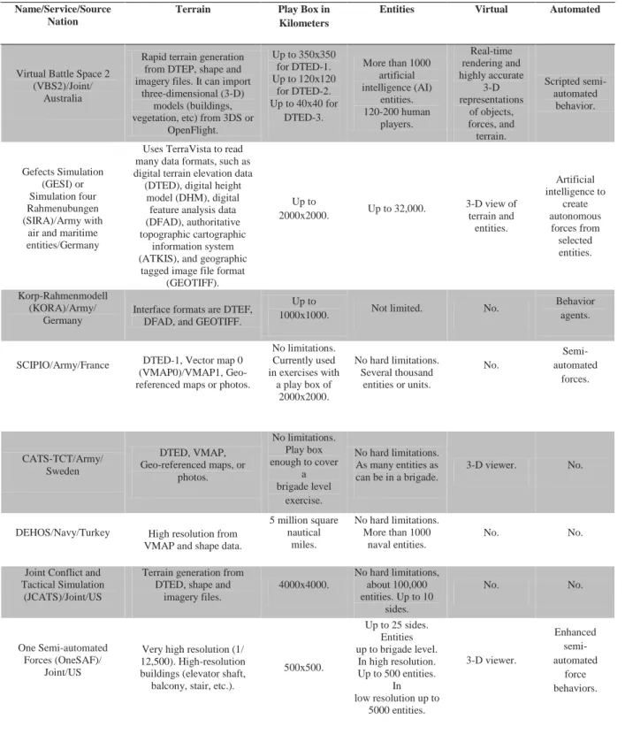
Table 1. High-resolution constructive simulation systems.

Name/Service/Source Nation

Terrain Play Box in

Kilometers

Entities Virtual Automated

Virtual Battle Space 2 (VBS2)/Joint/

Australia

Rapid terrain generation from DTEP, shape and imagery files. It can import

three-dimensional (3-D) models (buildings, vegetation, etc) from 3DS or

OpenFlight. Up to 350x350 for DTED-1. Up to 120x120 for DTED-2. Up to 40x40 for DTED-3. More than 1000 artificial intelligence (AI) entities. 120-200 human players. Real-time rendering and highly accurate 3-D representations of objects, forces, and terrain. Scripted semi-automated behavior. Gefects Simulation (GESI) or Simulation four Rahmenubungen (SIRA)/Army with

air and maritime entities/Germany

Uses TerraVista to read many data formats, such as digital terrain elevation data (DTED), digital height

model (DHM), digital feature analysis data (DFAD), authoritative topographic cartographic

information system (ATKIS), and geographic

tagged image file format (GEOTIFF). Up to 2000x2000. Up to 32,000. 3-D view of terrain and entities. Artificial intelligence to create autonomous forces from selected entities. Korp-Rahmenmodell (KORA)/Army/ Germany

Interface formats are DTEF, DFAD, and GEOTIFF.

Up to

1000x1000. Not limited. No.

Behavior agents. SCIPIO/Army/France DTED-1, Vector map 0

(VMAP0)/VMAP1, Geo-referenced maps or photos.

No limitations. Currently used in exercises with a play box of 2000x2000. No hard limitations. Several thousand entities or units. No. Semi-automated forces. CATS-TCT/Army/ Sweden DTED, VMAP, Geo-referenced maps, or photos. No limitations. Play box enough to cover a brigade level exercise. No hard limitations. As many entities as can be in a brigade. 3-D viewer. No.

DEHOS/Navy/Turkey High resolution from VMAP and shape data.

5 million square nautical miles. No hard limitations. More than 1000 naval entities. No. No. Joint Conflict and

Tactical Simulation (JCATS)/Joint/US

Terrain generation from DTED, shape and

imagery files. 4000x4000. No hard limitations, about 100,000 entities. Up to 10 sides. No. No. One Semi-automated Forces (OneSAF)/ Joint/US

Very high resolution (1/ 12,500). High-resolution buildings (elevator shaft, balcony, stair, etc.).

500x500. Up to 25 sides. Entities up to brigade level. In high resolution. Up to 500 entities. In low resolution up to 5000 entities. 3-D viewer. Enhanced semi-automated force behaviors.

(27)

7

2.2. Highly Aggregated Constructive Simulations

Examples for the highly aggregated constructive simulation systems are listed in table 2, which is again far from being exhaustive.

The major difference visible to users between high-resolution and highly aggregated simulation systems is the representation of the terrain and environment. In highly aggregated systems, the play box is tessellated with either hexagons or squares, and each of these hexagons or squares represents the following:

 Terrain characteristics (i.e., forest, ocean, desert, etc.)

 Mobility characteristics (i.e., good, bad, no mobility, etc.)

 Altitude or depth

Fig. 2. Terrain representations in highly aggregated constructive simulations [38].

Moreover, the sides of these hexagons or squares are used to introduce obstacles like rivers, tank ditches, shores, minefields, and so on. For example, a river that can be an obstacle for the unit mobility must follow the edges of these geometric shapes. This approach may not look very realistic, and sometimes the results from simulation do not match with the maps and the data in C2 systems. For example, the real location of the river may be several kilometers different from a hexagon edge. Because the model uses the hexagon edge as an obstacle, a unit may stuck somewhere that does not look realistic.

(28)

8

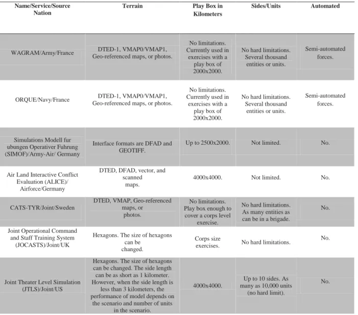
Table 2. Highly aggregated constructive simulation systems.

Name/Service/Source Nation

Terrain Play Box in

Kilometers

Sides/Units Automated

WAGRAM/Army/France _{Geo-referenced maps, or photos.}DTED-1, VMAP0/VMAP1,

No limitations. Currently used in exercises with a play box of 2000x2000. No hard limitations. Several thousand entities or units. Semi-automated forces.

ORQUE/Navy/France DTED-1, VMAP0/VMAP1, Geo-referenced maps, or photos.

No limitations. Currently used in exercises with a play box of 2000x2000. No hard limitations. Several thousand entities or units. Semi-automated forces.

Simulations Modell fur ubungen Operativer Fuhrung (SIMOF)/Army-Air/ Germany

Interface formats are DFAD and GEOTIFF.

Up to 2500x2000. Not limited. No. Air Land Interactive Conflict

Evaluation (ALICE)/ Airforce/Germany

DTED, DFAD, vector, and scanned

maps.

4000x4000. Not limited. No. CATS-TYR/Joint/Sweden

DTED, VMAP, Geo-referenced maps, or

photos.

No limitations. Play box enough to

cover a corps level exercise.

No hard limitations. As many entities as can be in a brigade.

No. Joint Operational Command

and Staff Training System (JOCASTS)/Joint/UK

Hexagons. The size of hexagons can be

changed.

Corps size

exercises. No hard limitations.

No.

Joint Theater Level Simulation (JTLS)/Joint/US

Hexagons. The size of hexagons can be changed. The side length can be as short as 1 kilometer. However, when the side length is

less than 3 kilometers, the performance of model depends on

the scenario and number of units in the scenario.

4000x4000.

Up to 10 sides. As many as 10,000 units

(no hard limit).

(29)

9

Approach

This thesis will explore current, and introduce new techniques with the aim of improving the reliability of warfare computer simulation. Such techniques can bring significant advantages in numerous real life scenarios.

After reviewing the state-of-the-art, we reach the conclusion that none of solutions addressed this matter in an efficient way. Also, there is not much information about them as they are closed systems used by governments to simulate battlefield scenarios.

Accordingly, this thesis proposes a new simulation meta-heuristic based on an evolutionary approach with the use of evolutionary algorithms. This meta-heuristic will behave, much as possible, as the military would do in the battlefield. And mainly will be opened to everyone.

3.1. Design challenges and considerations

Warfare simulation, while theoretically a very attractive proposition, faces additional design and implementation hurdles when compared to other types of simulation. Thus, special care must be taken when designing a meta-heuristic which purpose is to simulate the battlefield.

3.1.1. Problem Complexity

Computational complexity is a branch of the theory of computation in theoretical computer science and mathematics that focuses on classifying computational problems according to their inherent difficulty. In this context, a computational problem is understood

(30)

10

to be a task that is in principle possible of being solved by a computer (which basically means that the problem can be stated by a set of mathematical instructions). Informally, a computational problem consists of problem instances and solutions to these problem instances. For example, primality testing is the problem of determining whether a given number is prime or not. The instances of this problem are natural numbers, and the solution to an instance is yes or no based on whether the number is prime or not.

A problem is regarded as inherently difficult if its solution requires significant resources, whatever the algorithm used. The theory formalizes this intuition, by introducing mathematical models of computation to study these problems and quantifying the amount of resources needed to solve them, such as time and storage. One of the roles of computational complexity theory is to determine the practical limits on what computers can and cannot do.

Closely related fields in theoretical computer science are analysis of algorithms and computability theory. A key distinction between analysis of algorithms and computational complexity theory is that the former is devoted to analyzing the amount of resources needed by a particular algorithm to solve a problem, whereas the latter asks a more general question about all possible algorithms that could be used to solve the same problem. More precisely, it tries to classify problems that can or cannot be solved with appropriately restricted resources. In turn, imposing restrictions on the available resources is what distinguishes computational complexity from computability theory: the latter theory asks what kind of problems can, in principle, be solved algorithmically.

 Complexity classes

 What is a complexity class?

Typically, a complexity class is defined by (1) a model of computation, (2) a resource (or collection of resources), and (3) a function known as the complexity bound for each resource [40].

The models used to define complexity classes fall into two main categories: (1) machine-based models, and (2) circuit-machine-based models. Turing machines (TMs) and random-access machines (RAMs) are the two principal families of machine models. There are different kinds of (Turing) machines, such deterministic, non-deterministic, alternating, and oracle machines which are out of the scope of this thesis.

(31)

11

When there is the necessity to model real computations, deterministic machines and circuits are our closest links to reality. Then why consider the other kinds of machines? There are two main reasons.

The most potent reason comes from the computational problems whose complexity we are trying to understand. The most notorious examples are the hundreds of natural NP-complete problems [1]. To the extent that we understand anything about the complexity of these problems, it is because of the model of non-deterministic Turing machines. Non-deterministic machines do not model physical computation devices, but they do model real computational problems. There are many other examples where a particular model of computation has been introduced in order to capture some well-known computational problem in a complexity class. The second reason is related to the first. Our desire to understand real computational problems has forced upon us a repertoire of models of computation and resource bounds. In order to understand the relationships between these models and bounds, we combine and mix them and attempt to discover their relative power. Consider, for example, non-determinism. By considering the complements of languages accepted by non-deterministic machines, researchers were naturally led to the notion of alternating machines. When alternating machines and deterministic machines were compared, a surprising virtual identity of deterministic space and alternating time emerged.

Subsequently, alternation was found to be a useful way to model efficient parallel computation. This phenomenon, whereby models of computation are generalized and modified in order to clarify their relative complexity, has occurred often through the brief history of complexity theory, and has generated some of the most important new insights [41].

Other underlying principles in complexity theory emerge from the major theorems showing relationships between complexity classes. These theorems fall into two broad categories. Simulation theorems show that computations in one class can be simulated by computations that meet the defining resource bounds of another class. The containment of non-deterministic logarithmic space (NL) in polynomial time (P), and the equality of the class P with alternating logarithmic space, are simulation theorems. Separation theorems show that certain complexity classes are distinct.

(32)

12

Complexity theory currently has precious few of these. The main tool used in those separation theorems we have is called diagonalization. This ties in to the general feeling in computer science that lower bounds are hard to prove. Our current inability to separate many complexity classes from each other is perhaps the greatest challenge posed by computational complexity theory.

 Time and Space Complexity Classes

Fundamental time classes and fundamental space classes, given functions and :

1. is the class of languages decided by deterministic Turing machines of

time complexity ;

2. is the class of languages decided by non-deterministic Turing machines

of time complexity t(n);

3. is the class of languages decided by deterministic Turing machines of

space complexity ;

4. is the class of languages decided by non-deterministic Turing

machines of space complexity .

 Canonical Complexity Classes

Table 3. Canonical Complexity Classes

Complexity class Time/Space class decomposition Class Name

Deterministic log space

Non-deterministic log space

Polynomial time Non-deterministic polynomial time Polynomial space

Deterministic exponential time

Non-deterministic exponential

time

Exponential space

NP is the set of all decision problems for which the instances where the answer is ―yes‖ have efficiently verifiable proofs of the fact that the answer is indeed ―yes‖. More

(33)

13

precisely, these proofs have to be verifiable in polynomial time by a deterministic Turing machine. In an equivalent formal definition, NP is the set of decision problems where the ―yes‖ instances can be recognized in polynomial time by a non-deterministic Turing machine. The equivalence of the two definitions follows from the fact that an algorithm on such a non-deterministic machine consists of two phases, the first of which consists of a guess about the solution which is generated in a non-deterministic way, while the second consists of a deterministic algorithm which verifies or rejects the guess as a valid solution to the problem [2].

The complexity class P is contained in NP, but NP contains many important problems, the hardest of which are called NP-complete problems, for which no polynomial-time algorithms are known. The most important open question in complexity theory, the P = NP problem, asks whether such algorithms actually exist for NP-complete, and by corollary, all NP problems. It is widely believed that this is not the case [42].

As described before, the complexity class NP can be defined in terms of NTIME as follows:

(1)

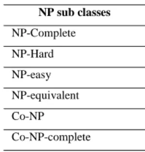
The NP class has several sub classes, as presented in table 4.

Table 4. NP Sub Classes

NP sub classes NP-Complete NP-Hard NP-easy NP-equivalent Co-NP Co-NP-complete

(34)

14

 NP-Hard

NP-hard (non-deterministic polynomial-time hard), is a class of problems that are, informally, ―at least as hard as the hardest problems in NP‖. A problem H is NP-hard if and only if there is an NP-complete problem that is polynomial time Turing-reducible to (i.e.,

TH). In other words, L can be solved in polynomial time by an oracle machine with an

oracle for . Informally, we can think of an algorithm that can call such an oracle machine as

a subroutine for solving , and solves in polynomial time, if the subroutine call takes only

one step to compute. NP-hard problems may be of any type: decision problems, search problems, or optimization problems.

As consequences of definition (note that these are claims, not definitions) [43]:

 Problem is at least as hard as , because can be used to solve ;

 Since is NP-complete, and hence the hardest in class NP, also problem is at

least as hard as NP, but does not have to be in NP and hence does not have to be a decision problem (even if it is a decision problem, it need not be in NP);

 Since NP-complete problems transform to each other by polynomial-time many-one reduction (also called polynomial transformation), all NP-complete problems

can be solved in polynomial time by a reduction to , thus all problems in NP

reduce to ; note, however, that this involves combining two different

transformations: from NP-complete decision problems to NP-complete problem

by polynomial transformation, and from to H by polynomial Turing reduction;  If there is a polynomial algorithm for any NP-hard problem, then there are

polynomial algorithms for all problems in NP, and hence ;

 If , then NP-hard problems have no solutions in polynomial time, while

does not resolve whether the NP-hard problems can be solved in polynomial time;

 If an optimization problem has an NP-complete decision version , then is

NP-hard.

A common mistake is to think that the NP in NP-hard stands for non-polynomial. Although it is widely suspected that there are no polynomial-time algorithms for NP-hard

(35)

15

problems, this has never been proven. Moreover, the class NP also contains all problems which can be solved in polynomial time.

The traditional lines of attack for NP-hard problems are the Following:

 Devising algorithms for finding exact solutions (they will work reasonably fast only for relatively small problem sizes);

 Devising ―suboptimal‖ or heuristic algorithms, i.e., algorithms that deliver either seemingly or probably good solutions, but which could not be proved to be optimal; Such algorithms can be: genetic algorithms, tabu search, ant algorithms, among others.  Finding special cases for the problem (―sub problems‖) for which either better or exact

algorithms are available.

 The Units Movement case

In this case the goal is to minimize the total movement cost between the targets having to pass to each one of them; this case is similar to the traveling salesman problem. So, one wants the best path which corresponds to a sequence of targets. In order to enumerate the set of paths, first is chosen one target, then another one, and so on.

Number of different paths: If is the number of targets, then, at each step there can be chosen between targets.

So,

Complexity: The complexity is . As expected, this approach leads to an

(hyper-)exponential algorithm. (the factorial function is hyper-exponential:

(36)

16

The best route is DACBE costing 185.

Complexity of verification: If a solution (i.e. a sequence of targets) is given, how long is it to compute its cost?

Only one path to explore, with targets, so the complexity of verification is

linear: .

So, this case is in NP and is hard because it is an optimization problem with the objective of finding the least-cost path through all the targets of a weighted map and the decision problem (―given the cost and a number x, decide whether there is a path cheaper than x‖) is NP-Complete. If there was a non-deterministic Turing machine, all the paths could be explored in one go, with linear complexity.

Following this reasoning, the complexity of this optimization involves at least one NP-hard problem making it NP-NP-hard.

3.1.2. Multi-objective optimization

For multiple-objective problems, the objectives are generally conflicting, preventing simultaneous optimization of each objective. Many, or even most, real engineering problems

(37)

17

actually do have multiple objectives, i.e., minimize cost, maximize performance, maximize reliability, etc. These are difficult but realistic problems. EAs are a popular meta-heuristic that is particularly well-suited for this class of problems. Traditional EAs are customized to accommodate multi-objective problems by using specialized fitness functions and introducing methods to promote solution diversity.

There are two general approaches to multiple-objective optimization. One is to combine the individual objective functions into a single composite function or move all but one objective to the constraint set. In the former case, determination of a single objective is possible with methods such as utility theory, weighted sum method, etc., but the problem lies in the proper selection of the weights or utility functions to characterize the decision-maker‘s preferences.

In practice, it can be very difficult to precisely and accurately select these weights, even for someone familiar with the problem domain. Compounding this drawback is that scaling amongst objectives is needed and small perturbations in the weights can sometimes lead to quite different solutions. In the latter case, the problem is that to move objectives to the constraint set, a constraining value must be established for each of these former objectives.

This can be rather arbitrary. In both cases, an optimization method would return a single solution rather than a set of solutions that can be examined for trade-offs [44]. For this reason, decision-makers often prefer a set of good solutions considering the multiple objectives.

The second general approach is to determine an entire Pareto optimal solution set or a representative subset. A Pareto optimal set is a set of solutions that are non-dominated with respect to each other. While moving from one Pareto solution to another, there is always a certain amount of sacrifice in one objective(s) to achieve a certain amount of gain in the other(s). Pareto optimal solution sets are often preferred to single solutions because they can be practical when considering real-life problems since the final solution of the decision-maker is always a trade-off. Pareto optimal sets can be of varied sizes, but the size of the Pareto set usually increases with the increase in the number of objectives.

(38)

18

 Multi-objective optimization formulation

Consider a decision-maker who wishes to optimize objectives such that the objectives

are non-commensurable and the decision-maker has no clear preference of the objectives relative to each other. Without loss of generality, all objectives are of the minimization type — a minimization type objective can be converted to a maximization type by multiplying

negative one. A minimization multi-objective decision problem with objectives is defined

as follows:

Given an -dimensional decision variable vector in the solution space ,

find a vector that minimizes a given set of objective functions

. The solution space is generally restricted by a series of

constraints, such as for , and bounds on the decision variables.

In many real-life problems, objectives under consideration conflict with each other.

Hence, optimizing with respect to a single objective often results in unacceptable results

with respect to the other objectives. Therefore, a perfect multi-objective solution that simultaneously optimizes each objective function is almost impossible. A reasonable solution to a multi-objective problem is to investigate a set of solutions, each of which satisfies the objectives at an acceptable level without being dominated by any other solution.

If all objective functions are for minimization, a feasible solution is said to dominate

another feasible solution , if and only if, for and

for least one objective function . A solution is said to be Pareto optimal if it is not dominated by any other solution in the solution space. A Pareto optimal solution cannot be improved with respect to any objective without worsening at least one other objective. The set

of all feasible non-dominated solutions in is referred to as the Pareto optimal set, and for a

given Pareto optimal set, the corresponding objective function values in the objective space are called the Pareto front. For many problems, the number of Pareto optimal solutions is enormous (perhaps infinite) [45].

The ultimate goal of a multi-objective optimization algorithm is to identify solutions in the Pareto optimal set. However, identifying the entire Pareto optimal set, for many multi-objective problems, is practically impossible due to its size. In addition, for many problems,

(39)

19

especially for combinatorial optimization problems, proof of solution optimality is computationally infeasible. Therefore, a practical approach to multi-objective optimization is to investigate a set of solutions (the best-known Pareto set) that represent the Pareto optimal set as well as possible. With these concerns in mind, a multi-objective optimization approach should achieve the following three conflicting goals [3]:

1. The best-known Pareto front should be as close as possible to the true Pareto front. Ideally, the best-known Pareto set should be a subset of the Pareto optimal set;

2. Solutions in the best-known Pareto set should be uniformly distributed and diverse over of the Pareto front in order to provide the decision-maker a true picture of trade-offs;

3. The best-known Pareto front should capture the whole spectrum of the Pareto front. This requires investigating solutions at the extreme ends of the objective function space.

For a given computational time limit, the first goal is best served by focusing (intensifying) the search on a particular region of the Pareto front. On the contrary, the second goal demands the search effort to be uniformly distributed over the Pareto front. The third goal aims at extending the Pareto front at both ends, exploring new extreme solutions.

(40)

(41)

21

Background Canonical Models

4.1. Supporting procedures and mechanisms

As stated before the problem which we are trying to solve with the meta-heuristic described later in this thesis is somehow complex and demanding, so there are several well known canonical models and algorithms used for solving the problem which are described in this section. This section aims that the reader understands all the terms and algorithm principles used throughout the thesis, although it is not exhaustive.

4.1.1. Evolutionary algorithms

 Aims of this section

The most important aim of this section is to describe what an Evolutionary Algorithm (EA) is. This description is deliberately based on a unifying view presenting a general scheme that forms the common basis of all Evolutionary Algorithm variants. The main components of EAs are discussed, explaining their role and related issues of terminology. Further on the general issues for EAs are discussed concerning their working. Finally, EAs are put into a broader context and their relation is explained with other global optimization techniques.

 What is an Evolutionary Algorithm?

As the history of the field suggests there are many different variants of EAs. The common underlying idea behind all these techniques is the same: given a population of individuals the environmental pressure causes natural selection (survival of the fittest) and

(42)

22

this causes a rise in the fitness of the population. Given a quality function to be maximized we can randomly create a set of candidate solutions, i.e., elements of the function's domain, and apply the quality function as an abstract fitness measure - the higher the better. Based on this fitness, some of the better candidates are chosen to seed the next generation by applying recombination and/or mutation to them. Recombination is an operator applied to two or more selected candidates (the so-called parents) and results one or more new candidates (the children). Mutation is applied to one candidate and results in one new candidate.

Executing recombination and mutation leads to a set of new candidates (the offspring) that compete - based on their fitness (and possibly age) - with the old ones for a place in the next generation. This process can be iterated until a candidate with sufficient quality (a solution) is found or a previously set computational limit is reached. In this process there are two fundamental forces that form the basis of evolutionary systems.

 Variation operators (recombination and mutation) create the necessary diversity and

thereby facilitate novelty, while

 selection acts as a force pushing quality.

The combined application of variation and selection generally leads to improving fitness values in consecutive populations. It is easy (although somewhat misleading) to see such a process as if the evolution is optimizing, or at least ―approximating‖, by approaching optimal values closer and closer over its course. Alternatively, evolution it is often seen as a process of adaptation.

From this perspective, the fitness is not seen as an objective function to be optimized, but as an expression of environmental requirements. Matching these requirements more closely implies an increased viability, reflected in a higher number of offspring. The evolutionary process makes the population adapt to the environment better and better.

Note that many components of such an evolutionary process are stochastic. During selection fitter individuals have a higher chance to be selected than less fit ones, but typically even the weak individuals have a chance to become a parent or to survive. For recombination of individuals the choice of which pieces will be recombined is random. Similarly for mutation, the pieces that will be mutated within a candidate solution, and the new pieces

(43)

23

replacing them, are chosen randomly. The general scheme of an EA can is given in listing 1 in a pseudo-code fashion; figure 3 shows a diagram.

It is easy to see that this scheme falls in the category of generate-and-test algorithms. The evaluation (fitness) function represents a heuristic estimation of solution quality and the search process is driven by the variation and the selection operators. EAs posses a number of features that can help to position them within in the family of generate-and-test methods:

 EAs are population based, i.e., they process a whole collection of candidate solutions

simultaneously;

 EAs mostly use recombination to mix information of more candidate solutions into a

new one;

 EAs are stochastic1.

1

Stochastic refers to systems whose behavior is intrinsically non-deterministic. A stochastic process is one whose behavior is non-deterministic, in that a system's subsequent state is determined both by the process's predictable actions and by a random element.

BEGIN

INITIALIZE population with random candidate solutions; EVALUATE each candidate;

REPEAT UNTIL (TERMINATION CONDITION is satisfied) DO 1 SELECT parents;

2 RECOMBINE pairs of parents; 3 MUTATE the resulting offspring; 4 EVALUATE new candidates;

5 SELECT individuals for the next generation; END REPEAT

END

Fig. 4. The general scheme of an Evolutionary Algorithm as a flow-chart [46]. Listing 1. Pseudo-code of an EA general scheme

(44)

24

The various dialects of evolutionary computing that were mentioned previously all follow the general outlines in figure 4, and differ only in technical details. For instance, the representation of a candidate solution is often used to characterize different streams. Typically, the candidates are represented by (i.e., the data structure encoding a solution has the form of) strings over a finite alphabet in Genetic Algorithms (GA), real-valued vectors in Evolution Strategies (ES), finite state machines in classical Evolutionary Programming (EP) and trees in Genetic Programming (GP). These differences have a mainly historical origin. Technically, a given representation might be preferable over others if it matches the given problem better, that is, it makes the encoding of candidate solutions easier or more natural. For instance, for solving a satisfiability problem the straightforward choice is to use

bit-strings of length , where is the number of logical variables, hence the appropriate EA

would be a Genetic Algorithm.

For evolving a computer program that can play checkers, trees are well-suited (namely, the parse trees of the syntactic expressions forming the programs), thus a GP approach is likely. It is important to note that the recombination and mutation operators working on candidates must match the given representation. Thus for instance in GP the recombination operator works on trees, while in GAs it operates on strings. As opposed to variation operators, selection takes only the fitness information into account, hence it works independently from the actual representation. Differences in the commonly applied selection mechanisms in each stream are therefore rather a tradition than a technical necessity.

 Components of Evolutionary Algorithms

In this section is discussed EAs in detail. EAs have a number of components, procedures or operators that must be specified in order to define a particular EA. The most important components, indicated by italics in listing 1, are:

 representation (definition of individuals);

 evaluation function (or fitness function);

 population;

 parent selection mechanism;

(45)

25

 survivor selection mechanism (replacement).

Each of these components must be specified in order to define a particular EA. Furthermore, to obtain a running algorithm the initialization procedure and a termination condition must be also defined.

 Representation (Definition of Individuals)

The first step in defining an EA is to link the ―real world‖ to the ―EA world‖, that is to set up a bridge between the original problem context and the problem solving space where evolution will take place. Objects forming possible solutions within the original problem context are referred to as phenotypes, their encoding, the individuals within the EA, are called genotypes. The first design step is commonly called representation, as it amounts to specifying a mapping from the phenotypes onto a set of genotypes that are said to represent these phenotypes. For instance, given an optimization problem on integers, the given set of integers would form the set of phenotypes. Then one could decide to represent them by their binary code, hence 18 would be seen as a phenotype and 10010 as a genotype representing it. It is important to understand that the phenotype space can be very different from the genotype space, and that the whole evolutionary search takes place in the genotype space. A solution - a good phenotype - is obtained by decoding the best genotype after termination. To this end, it should hold that the (optimal) solution to the problem at hand - a phenotype - is represented in the given genotype space.

The common EC terminology uses many synonyms for naming the elements of these two spaces. On the side of the original problem context, candidate solution, phenotype, and individual are used to denote points of the space of possible solutions. This space itself is commonly called the phenotype space. On the side of the EA, genotype, chromosome, and again individual can be used for points in the space where the evolutionary search will actually take place. This space is often termed the genotype space. Also for the elements of individuals there are many synonymous terms. A place-holder is commonly called a variable, a locus (plural: loci), a position, or - in a biology oriented terminology - a gene. An object on such a place can be called a value or an allele.

(46)

26

It should be noted that the word ―representation‖ is used in two slightly different ways. Sometimes it stands for the mapping from the phenotype to the genotype space. In this sense it is synonymous with encoding, i.e., one could mention binary representation or binary encoding of candidate solutions [47]. The inverse mapping from genotypes to phenotypes is usually called decoding and it is required that the representation be invertible: to each genotype there has to be at most one corresponding phenotype. The word representation can also be used in a slightly different sense, where the emphasis is not on the mapping itself, but on the ―data structure‖ of the genotype space. This interpretation is behind speaking about mutation operators for binary representation, for instance.

 Evaluation Function (Fitness Function)

The role of the evaluation function is to represent the requirements to adapt to. It forms the basis for selection, and thereby it facilitates improvements. More accurately, it defines what improvement means. From the problem solving perspective, it represents the task to solve in the evolutionary context. Technically, it is a function or procedure that assigns a quality measure to genotypes. Typically, this function is composed from a quality measure in the phenotype space and the inverse representation. To remain with the above example, if the

goal was to maximize on integers, the fitness of the genotype 10010 could be defined as

the square of its corresponding phenotype: .

The evaluation function is commonly called the fitness function in EC. This might cause a counterintuitive terminology if the original problem requires minimization for fitness is usually associated with maximization. Mathematically, however, it is trivial to change minimization into maximization and vice versa.

Quite often, the original problem to be solved by an EA is an optimization problem. In this case the name objective function is often used in the original problem context and the evaluation (fitness) function can be identical to, or a simple transformation of, the given objective function.

(47)

27

 Population

The role of the population is to hold (the representation of) possible solutions. A

population is a multiset2 of genotypes [48]. The population forms the unit of evolution.

Individuals are static objects not changing or adapting, it is the population that does. Given a representation, defining a population can be as simple as specifying how many individuals are in it, that is, setting the population size. In some sophisticated EAs a population has an additional spatial structure, with a distance measure or a neighborhood relation. In such cases the additional structure has to be defined as well to fully specify a population. As opposed to variation operators that act on the one or two parent individuals, the selection operators (parent selection and survivor selection) work at population level. In general, they take the whole current population into account and choices are always made relative to what we have. For instance, the best individual of the given population is chosen to seed the next generation, or the worst individual of the given population is chosen to be replaced by a new one. In almost all EA applications the population size is constant, not changing during the evolutionary search.

The diversity of a population is a measure of the number of different solutions present. No single measure for diversity exists, typically people might refer to the number of different fitness values present, the number of different phenotypes present, or the number of different genotypes. Other statistical measures, such as entropy, are also used. Note that only one fitness value does not necessarily imply only one phenotype is present, and in turn only one phenotype does not necessarily imply only one genotype. The reverse is however not true: one genotype implies only one phenotype and fitness value.

 Parent Selection Mechanism

The role of parent selection or mating selection is to distinguish among individuals based on their quality, in particular, to allow the better individuals to become parents of the next generation. An individual is a parent if it has been selected to undergo variation in order to create offspring. Together with the survivor selection mechanism, parent selection is responsible for pushing quality improvements. In EC, parent selection is typically probabilistic. Thus, high quality individuals get a higher chance to become parents than those

(48)

28

with low quality. Nevertheless, low quality individuals are often given a small, but positive chance, otherwise the whole search could become too greedy and get stuck in a local optimum.

 Variation Operators

The role of variation operators is to create new individuals from old ones. In the corresponding phenotype space this amounts to generating new candidate solutions. From the generate-and-test search perspective, variation operators perform the ―generate‖ step.

Variation operators in EC are divided into two types based on their arity3 [49].

 Mutation

A unary4 variation operator is commonly called mutation. It is applied to one genotype

and delivers a (slightly) modified mutant, the child or offspring of it. A mutation operator is always stochastic: its output - the child - depends on the outcomes of a series of random

choices5. It should be noted that an arbitrary unary operator is not necessarily seen as

mutation. A problem specific heuristic operator acting on one individual could be termed as mutation for being unary. However, in general mutation is supposed to cause a random, unbiased change. For this reason it might be more appropriate not to call heuristic unary operators mutation. The role of mutation in EC is different in various EC-dialects, for instance in Genetic Programming it is often not used at all, in Genetic Algorithms it has traditionally been seen as a background operator to fill the gene pool with ―fresh blood‖, while in Evolutionary Programming it is the one and only variation operator doing the whole search work.

It is worth noting that variation operators form the evolutionary implementation of the elementary steps within the search space. Generating a child amounts to stepping to a new point in this space. From this perspective, mutation has a theoretical role too: it can guarantee that the space is connected. This is important since theorems stating that an EA will (given

3

The arity of an operator is the number of objects that it takes as inputs.

4_{An operator is unary if it applies to one object as input.}

5

Usually these will consist of using a pseudo-random number generator to generate a series of values from some given probability distribution. These can sometimes be referred as ―random drawings‖.

(49)

29

sufficient time) discover the global optimum of a given problem often rely on the property that each genotype representing a possible solution can be reached by the variation operators [55]. The simplest way to satisfy this condition is to allow the mutation operator to ―jump‖ everywhere, for example, by allowing that any allele can be mutated into any other allele with a non-zero probability. However it should also be noted that many researchers feel these proofs have limited practical importance, and many implementations of EAs do not in fact possess this property.

 Recombination

A binary variation operator6 is called recombination or crossover. As the names

indicate such operator merges information from two parent genotypes into one or two offspring genotypes. Similarly to mutation, recombination is a stochastic operator: the choice of what parts of each parent are combined, and the way these parts are combined, depends on random drawings.

Again, the role of recombination is different in EC dialects: in Genetic Programming it is often the only variation operator, in Genetic Algorithms it is seen as the main search operator, and in Evolutionary Programming it is never used. Recombination operators with a higher arity (using more than two parents) are mathematically possible and easy to

implement, but have no biological equivalent. Perhaps this is why they are not commonly

used, although several studies indicate that they have positive effects on the evolution [56].

The principal behind recombination is simple - that by mating two individuals with different but desirable features, we can produce an offspring which combines both of those features. This principal has a strong supporting case - it is one which has been successfully applied for millennia by breeders of plants and livestock, to produce species which give higher yields or have other desirable features. EAs create a number of offspring by random recombination, accept that some will have undesirable combinations of traits, most may be no better or worse than their parents, and hope that some have improved characteristics. Although the biology of the planet earth, (where with a very few exceptions lower organisms reproduce asexually, and higher organisms reproduce sexually), suggests that recombination

6

(50)

30

is the superior form of reproduction, recombination operators in EAs are usually applied probabilistically, that is, with an existing chance of not being performed.

It is important to note that variation operators are representation dependent. That is, for different representations different variation operators have to be defined. For example, if genotypes are bit-strings, then inverting a 0 to a 1 (1 to a 0) can be used as a mutation operator. However, if possible solutions are represented by tree-like structures another mutation operator is required.

 Survivor Selection Mechanism (Replacement)

The role of survivor selection or environmental selection is to distinguish among individuals based on their quality. In that it is similar to parent selection, but it is used in a different stage of the evolutionary cycle. The survivor selection mechanism is called after having created the offspring of the selected parents. As mentioned in the ―Population‖ section, in EC the population size is (almost always) constant, thus a choice has to be made on which individuals will be allowed in the next generation. This decision is usually based on their fitness values, favoring those with higher quality, although the concept of age is also frequently used. As opposed to parent selection which is typically stochastic, survivor selection is often deterministic, for instance ranking the unified multiset of parents and offspring and selecting the top segment (fitness biased), or selecting only from the offspring (age-biased).

Survivor selection is also often called replacement or replacement strategy. In many cases the two terms can be used interchangeably. The choice between the two is thus often arbitrary. A good reason to use the name survivor selection is to keep terminology consistent: step 1 and step 5 in Figure 4 are both named selection, distinguished by an adjective. A preference for using replacement can be motivated by the skewed proportion of the number of individuals in the population and the number of newly created children. In particular, if the number of children is very small with respect to the population size, i.e., 2 children and a population of 100. In this case, the survivor selection step is as simple as to choose the two old individuals that are to be deleted to make place for the new ones. In other words, it is more efficient to declare that everybody survives unless deleted, and to choose whom to