Abstract – This paper aims to analyze the spatial distribution of coffee productivity as well as to investigate whether there is a convergence process among the microregions of the five largest pro-ducing states of Brazil between 2000 and 2015. In order to do this, we used exploratory spatial data analysis (ESDA) and spatial econometrics. The main result indicate that microregions with low productivity are reaching very slowly the most dynamic regions, a fact that can adversely affect the economic and social development of these localities. Finally, we discuss the impacts of this slow convergence process on regional development and highlight some policies that can promote pro-ductivity improvements.
Keywords: exploratory spatial data analysis (ESDA), spatial convergence, spatial econometrics.
Produtividade do café e desenvolvimento regional no Brasil
Resumo – O objetivo deste trabalho é analisar a distribuição espacial da produtividade do café e investigar se há um processo de convergência entre as microrregiões dos cinco maiores produtores do Brasil de 2000 a 2015. Foram usadas a análise exploratória de dados espaciais (Aede) e a eco-nometria espacial. O principal resultado indicou que microrregiões com baixa produtividade estão convergindo numa velocidade lenta para as regiões mais dinâmicas, fato que pode afetar de forma adversa o desenvolvimento econômico e social destas. Discutem-se os impactos para o desenvol-vimento regional desse ritmo lento de convergência e destacam-se algumas políticas que podem gerar ganhos de produtividade.
Palavras-chave: análise exploratória de dados espaciais (Aede), convergência espacial, econometria espacial.
Coffee productivity
and regional
development in Brazil
1
1 Original recebido em 14/1/2019 e aprovado em 31/3/2019. 2 Doutorando em Economia. E-mail: [email protected]
3 Doutor em Economia Aplicada. E-mail: [email protected] 4 Bolsista de Iniciação Científica. E-mail: [email protected]
Pedro Henrique Batista de Barros2
Renato Alves de Oliveira3
Isadora Salvalaggio Baggio4
Introduction
Brazil stands out in the world coffee mar-ket as the largest producer of this commodity, a position held for more than a century. Coffee is important for Brazilian economic and social
history since the beginning of the 19th century, when its planting began in the country. Around 1830, coffee was already the main Brazilian export product, position maintained until the 1960s. The generation of wealth and foreign
the spatial distribution and possible adjacent spatial processes, namely the existence of spatial dependence and heterogeneity. In addition, for spatial convergence, we based on the Baumol’s seminal work (1986), which sought to examine the existence of convergence of per capita income among sixteen industrialized countries between 1870 and 1979.The equation used by Baumol (1986) is
ln(Y / N)i,t - ln(Y / N)i,t-1 = a + b ln(Y / N)i,t-1 + ei (1) where is the natural logarithm of per capita income, is the index for countries, and is the er-ror term. According to Baumol (1986), we have a convergence process when the b coefficient presents a negative signal and statistically signifi-cant coefficient. In other words, we investigated if the microregions with lower productivity had a higher growth rate. There are no papers in the literature that sought to investigate the coffee productivity convergence in a national scope, thus the present paper aims to fill this gap.
The spatial analysis techniques is an impor-tant tool in the present context, since agricultural exchange during this period allowed the country
to industrialize and develop economically, espe-cially in the import substitution period (Furtado, 2003).
Regarding domestic consumption, Brazil is currently the second largest consumer of cof-fee in the world, consuming approximately 1.23 million tons per year, which represents around 31% of the national production. These numbers suggests a per capita value of 5 kilograms of roasted and ground coffee or 81 liters. The rest of the country’s production, which corresponds to 1.782 million tons (69% of the total), is des-tined for export, mainly for the United States and Germany, with 19.03% and 18.30% of total, re-spectively (Cecafe, 2017). Although Brazil’s share of the world coffee market has dropped from 84% in the 1920s, a near-monopoly scenario, to one third in 2016, the country is still the world’s largest producer in the world (Iapar, 2017).
Given the importance of coffee produc-tion for Brazil, this paper aims to evaluate the coffee productivity performance in the country between 2000 and 2015, and its impact on re-gional development. We analyzed the five main coffee producing states of the country (MG, ES, SP, BA and PR), which concentrate the major part of national production. Figure 1 shows its location in the country and we can note a spatial concentration in the coffee´s production in the national scenario.
The best way to understand the evolution and performance of an agricultural commodity, according to Almeida et al. (2008), is to investi-gate how their average productivity behaved over time as well as seek evidence if it is converging spatially. In this context, this paper sought to ana-lyze the spatial distribution of coffee productivity, its dynamics in the period and the formation of clusters, among the 213 microregions that make up the five states. In addition, we estimated a spatial convergence (b convergence) model.
In order to reach the objectives, we used the techniques of Exploratory Analysis of Spatial Data (EASD), which make it possible to analyze
Figure 1. Microregions of the main coffee producing
states in Brazil.
activities are often subject to spatial effects. The existence of different production techniques, cli-mate, topography and soil conditions among the regions may induce significant regional differ-ences. Therefore, if such effects are not treated, any aggregate exploratory analysis or conven-tional econometric models may become biased and inconsistent. According to Quah (1996), the vast majority of convergence studies use regional data and are, therefore, spatial. However, the major part do not take into account possible spa-tial effects, which may invalidate the inferences. In addition, Rey & Montoury (1999) argues that procedures from ESDA and spatial economet-rics enabled more reliable and realistic estimates and inferences by allowing a new perspective on the geographical and spatial dynamics of growth over time between regions. Finally, we investigate the potential causes of productivity behavior and its impact on regional development, especially in the economic and social spheres. In addition, we highlight some policies and procedures that can promote productivity improvements, which can serve as guide agricultural policies develop-ment for the coffee sector in Brazil.
Convergence and spatial effects
We have some papers that focused on the Brazilian agriculture using the ESDA meth-odology. Perobelli et al. (2007) sought to map the spatial distribution of agricultural productiv-ity in Brazil in the period from 1990 to 2003. The author used the 558 microregions of the country and the main result is that agricultural productivity is spatially concentrated with two high clusters: one in São Paulo and in parts of the Central-West, while the other is located on the northeastern coast. Souza & Perobelli (2008), on the other hand, investigated the spatial distribu-tion of soybean crop for the same microregions in Brazil and found that this variable is also spa-tially autocorrelated.
Considering a spatial econometric ap-proach, we can highlight Rey & Montouri (1999) who estimated an income convergence model
for the American states in the period 1929 to 1994 using the Baumol (1986) specification. The authors’ innovation reflects their effort to con-sider the spatial aspects in their analysis by using spatial econometric methods. Rey & Montouri (1999) found evidence of spatial autocorrelation between American states and argues that the non-treatment of these effects in econometric modeling may lead to poor specification and consequent biases and inconsistency in the parameters.
For Brazil, we have some papers that estimated a b convergence model using spa-tial econometrics. For instance, Lopes (2004) analyzed the average agricultural productivity in Brazil and confirmed the spatial convergence hypothesis for some crops, such as coffee, sugar-cane, tobacco, manioc, orange, soybean, beans, potatoes and cotton. In addition, the author identifies that technological diffusions are impor-tant in explaining the convergence between land productivity.
Almeida et al. (2008), in turn, attempted to identify an absolute convergence for agricultural productivity in Brazil between 1991 and 2003. The author divided the period of analysis into three (1991-1994, 1995-1999 and 2000-2003) and they got a b convergence for 1991-1994 period, but not for 1995-1999 and 2000-2003. In any case, the 1991-1994 period was decisive to reduce the existing inequalities in agricultural productivity between the Brazilian regions.
Seeking to analyze the agricultural pro-ductivity evolution in the microregions of south-ern Brazil, Raiher et al. (2016) investigated the absolute and conditional convergence in the period 1995/96 to 2006. The authors found spa-tial dependence in the data; therefore, they used spatial-econometric models to estimate the con-vergence models. Raiher et al. (2016) found that agricultural productivity in the southern states in Brazil (PR, SC and RS) presented an absolute and conditional convergence. Teixeira & Bertella (2015) analyzed the absolute convergence for coffee average productivity in the Minas Gerais state, the Brazil’s largest producer. The authors
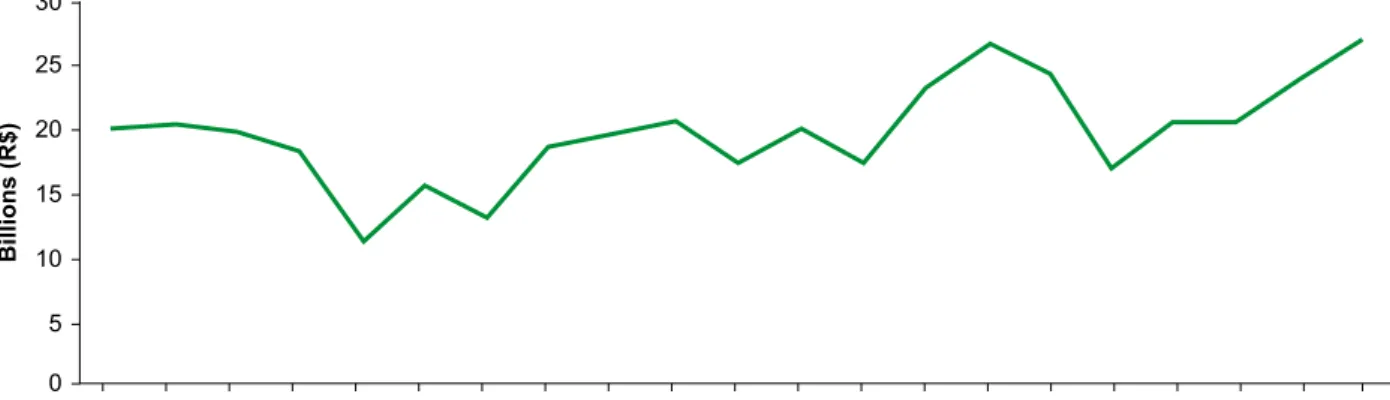
reaches R$ 24 billion. Therefore, we can note that the production showed only a small growth throughout the period, in addition to some instability.
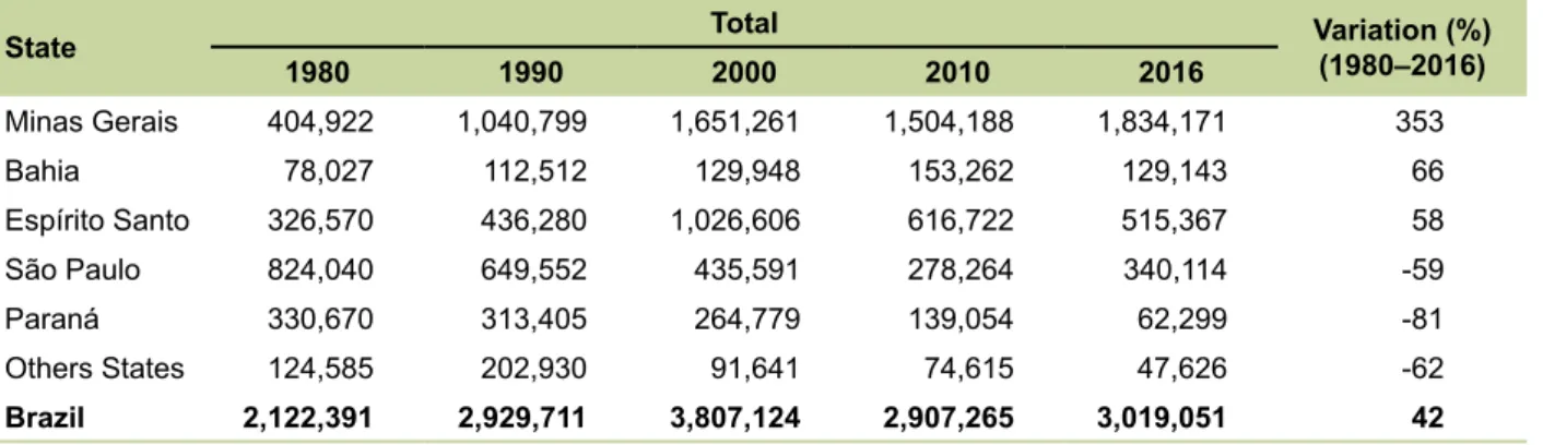
The coffee production distribution, in turn, are not homogeneous in the country, since it is concentrated in some Brazilian states. Table 1 shows the evolution of production in tons for the six main Brazilian producing states from 1980 to 2016. We can note that Minas Gerais (MG) be-came the largest national coffee producer in the period and presented a growth of 353%, from 404 thousand tons in 1980 to 1,834 thousand tons in 2016. The São Paulo (SP) state, which was the country’s largest producer in 1980, became the third largest producer in 2016, behind MG and Espírito Santo (ES), with a 59% reduction in its total production. The Paraná (PR), in turn, was the third largest producer in the country in 1980, but the state decrease 81% of its production in the period (the largest drop among the states considered) and now is the fifth largest producer
In order to better identify the relative posi-tion for which state and its evoluposi-tion since 1980, Table 2 shows the relative participation of the six largest coffee producers in Brazil. We can note that even between the largest producers, the production is concentrated, which has increased in recent periods. We can highlight the Minas Gerais case, which held 19% in 1980, after São used a microregional cut for 1997 to 2006 period
and identified, through an exploratory analysis of spatial data, the presence of spatial dependence in the data. In this context, they used a spatial econometric approach to model the conver-gence process. The results indicated an absolute convergence for the average coffee productivity in the state of Minas Gerais.
Brazilian coffee production
The Brazilian Agricultural Production Gross Value of (VBA) in 2016, according to IBGE (2017), are approximately R$ 523.00 billion, an amount of R$ 10.00 billion less than that pre-sented in 2015. This behaviour prepre-sented by Brazilian agriculture and cattle raising reflects the Brazilian economic crisis that began in 2014. When we considered the whole agribusiness sector GDP, which include inputs, primary production, agroindustry and services, the value reaches R$ 1,425.00 trillion in 2016. This result represents 23% of the R$ 6,188.00 trillion from the Brazilian GDP, a value that shows the agri-business importance for the country economy (CNA, 2017).
The coffee production in Brazil (Figure 2), on the other hand, presented only a modest evolution in the period between 1997 and 2017. For example, in 1997, the coffee production was about R$ 20 billion while in 2016 this amount
Figure 2. Coffee production (R$) between 1997 and 2017.
Table 1. The biggest Brazilian coffee producing states, in tons of grains, between 1980 and 2016.
State Total Variation (%) (1980–2016)
1980 1990 2000 2010 2016 Minas Gerais 404,922 1,040,799 1,651,261 1,504,188 1,834,171 353 Bahia 78,027 112,512 129,948 153,262 129,143 66 Espírito Santo 326,570 436,280 1,026,606 616,722 515,367 58 São Paulo 824,040 649,552 435,591 278,264 340,114 -59 Paraná 330,670 313,405 264,779 139,054 62,299 -81 Others States 124,585 202,930 91,641 74,615 47,626 -62 Brazil 2,122,391 2,929,711 3,807,124 2,907,265 3,019,051 42
Source: elaborated with data from IBGE (2017).
Paulo with 39%. In 2016, the state became the largest producer, with 61% of the country’s total production. On the other hand, the Paraná state has suffered a considerable reduction in its rela-tive share of coffee production from 16% in 1980 to 2% in 2016.
Table 2. Relative participation of the six main Brazilian coffee producing states.
State Relative participation (%)
1980 1990 2000 2010 2016 Minas Gerais 19 36 43 52 61 Espírito Santo 15 15 27 21 17 São Paulo 39 22 11 10 11 Bahia 4 4 3 5 4 Paraná 16 11 7 5 2 Others states 6 7 2 3 2
Source: elaborated with data from IBGE (2017).
The average coffee productivity in Brazil (Table 3) increased by 74% in the 1980 to 2016 period. However, we have a heterogeneity in the spatial distribution of this productivity increase. For example, the state that gained the most pro-ductivity are the Paraná state, followed by Minas
Table 3. Average productivity of coffee production (kg/ha).
State Productivity (kg/ha) Growth (%)
1980 1990 2000 2010 2016 Paraná 520 735 1,863 1,681 1,415 172 Minas Gerais 876 1,080 1,662 1,465 1,761 101 São Paulo 1,024 1,145 2,059 1,372 1,704 66 Espírito Santo 1,074 859 1,961 1,303 1,218 13 Bahia 879 825 1,117 1,007 790 -10 Brazil 872 1,007 1,678 1,346 1,513 74
Gerais. One possible explanation for the Paraná behavior is that the state started from a smaller base when compared to the others. Even with this gain in productivity, the state is still below the Brazilian average. Considering the fact that production in the state has fallen steeply, a con-siderable part of this increase may have been because the producers with low productivity left and those with greater not, which made the ave-rage productivity increase. In any case, a more careful investigation into the local dynamics are necessary.
As expected, the Minas Gerais state, the largest coffee producer in the country, has the highest average productivity in 2016. The São Paulo, in turn, presented the second largest and this state presented a similar dynamics of Paraná, because its relative share also fell considerably in the period despite the increase in productivity. Espírito Santo, on the other hand, presented only 13% of growth its average productivity, however, the state to maintain its relative share. Bahia had a different behavior from the others, as it decrea-sed its average productivity in the period.
Methodology
Exploratory Spatial Data
Analysis (ESDA)
The ESDA are techniques used to capture spatial dependence and heterogeneity in the data. For this reason, it is important in the model specification process, since if it indicates that there is some type of spatial process, we must incorporated into the model to avoid economet-ric problems such as bias and inconsistency in the parameters. ESDA is also able to capture, for example, spatial association patterns (spatial clusters), indicate how the data are distributed, presence of different spatial regimes or other forms of spatial instability (non-stationarity), and identify outliers (Anselin, 1995; Perobelli et al., 2007; Almeida, 2012).
Spatial dependence means that the vari-able in a region depends on the value of the same variable in other regions. This dependence occurs in all directions, but tends to decrease its impact as increases geographic distance. On the other hand, spatial heterogeneity is related to the regions characteristics and leads to structural in-stability. In other words, each locality may have a distinct response when exposed to the same influence (Almeida, 2012).
The first step is to test whether there is spatial autocorrelation between regions, in other words, whether the data are spatially dependent or randomly distributed. One way to verify this is through Moran’s I, which seeks to capture the
spatial correlation degree between the variable across regions. The expected value of this statis-tic is E(I) = -1 / (n - 1), if the values are statistically
higher or lower than expected, we have a positive or negative spatial autocorrelation respectively. Mathematically, we can represent by
It = (n / S0) (zt' Wzt / zt'zt) t = 1,...,n (2)
in which n is the number of regions, S0 is a value equal to the sum of all matrix W elements, z is the
variable normalized value;Wz is the normalized
variable mean value in neighbors according to a weighting matrix W.
However, the Moran’s I statistic, according
to Anselin (1995), can only capture the global autocorrelation, not identifying the spatial as-sociation at a local level. For this, we have complementary measures that aim to capture lo-cal spatial autocorrelation and seeks to observe local spatial clusters existence. The main are the LISA (Local Indicator of Spatial Association) statistic. For an indicator to be LISA, it must have two characteristics: (i) for each observation it should be possible to indicate the spatial clusters existence and significance; ii) the local indicators sum, in all places, should be proportional to the global spatial autocorrelation indicator. The local Moran I statistic (LISA) are
tial dependence on the model residuals, which is represented by
ln = (ProdCt / ProdCt-n) =
= a + b ln(ProdCt-n) + ei (4) where (ProdCt / ProdCt-n) is the natural logarithm of the ratio between the average coffee produc-tivity in the final and initial period of the micro-regions; b ln(ProdCt-n) is the natural logarithm of the average coffee productivity in the initial period; ei is the error term.
The absolute convergence hypothesis for coffee productivity between microregions are confirmed if the b convergence is significant and present a negative signal. This would mean that microregions that had a higher average produc-tivity in period t - 1 are presenting a lower growth
rate than when compared with those that started the period with smaller productivities rates. In the following paragraphs, based on Rey & Montoury (1999), we incorporate the spatial components in (4) and explain the possible interpretations for these variables in this paper context.
The Spatial Autoregressive Model (SAR) seeks to capture the spatial dependence from productivity growth rate between neighbor-ing microregions, in other words, the spatial interaction. Therefore, the dependent variable is spatially lagged and included as an explanatory variable in the econometric model, which can be interpreted as the mean value of the neighboring spatial units. Formally, we have
ln(ProdCt / ProdCt-n) = a + b ln(ProdCt-n) + + rW ln(ProdCt / ProdCt-n) + ei (5) in which r is the spatial lag coefficient. If sig-nificant and r > 0 there is a positive spatial autocorrelation effect. W ln(ProdCt / ProdCt-n) is the dependent variable spatial lag from the neighboring microregions. The model suffer from endogeneity of the lagged variable, and then we must estimate using instrumental variables, which are the lagged explanatory variables (WX). Ii = zi wij zj (3)
where zi represents the variable for the standard-ized region i, wij is the spatial weighting matrix element (W) and zj is the variable value in the standardized region j.
The ESDA provide information on the ex-istence of spatial dependence and heterogeneity for the phenomenon. If we have at least one of these spatial processes, the we should use spe-cific econometric techniques, known as Space Econometrics, to control these spatial effects.
Spatial convergence analysis
According to Almeida (2012), the spatial effects not consideration in econometric model-ing may violate some assumptions of the classical linear regression model, leading to biased and inefficient estimators along with heteroscedastic-ity. We incorporated the spatial component in the econometric model through spatially lagged variables. Among the lags used, we have the lag of the dependent variable, the explanatory variable (WX) and the error term (Wξ or We).
It is these variables that, when included in the model, control the spatial dependence present in the data.
The econometric models that include the lagged dependent variable (Wy) are the Spatial
Lag Model (SAR). The one that includes the error term (Wξ or We) are the Spatial Error Model (SEM)
and finally, the one that includes the spatial lag of the independent variable (WX) are the spatial
lag of X model (SLX). These are the most used
models in spatial econometric modeling. The choice of the model, however, does not occur arbitrarily, since spatial effects may be present in some variable or term of error and not in oth-ers. There are certain procedures to be adopted when choosing the best modeling for spatial ef-fects (Florax et al., 2003).
The first step is to estimate the absolute convergence b model by OLS to search for
spa-The spatial error model (SEM), in turn, is used when spatial dependence manifests itself in the error term. The non-inclusion of this spatial interaction in the econometric model can bias the estimates. Mathematically, we have
ln(ProdCt / ProdCt-n) = a + b ln(ProdCt-n) +
+ (I - lW)ξi (6)
ξi = lWξi + ei
in which l is the spatial error coefficient; ei is the error term with mean zero and constant variance. If l= 0, there is no indication of spatial autocor-relation in the error and closer to one is the pa-rameter, the greater is the shock in neighboring regions. The estimation by OLS is not adequate, since the bias in the error term makes the model parameters estimations inefficient. Therefore, according to Kelejian & Prucha (1999), we must estimate the SEM model by maximum likelihood (MV) or the generalized method of moments (MGM).
Finally, the Spatial lag of X Model (SLX) seeks to capture the spatial spillover from the in-dependent variable of neighboring microregions, using the spatial weights matrix W as a spatial lag
operator. This lag is exogenous, since the explana-tory variables are determined outside the model. For this reason, there are no endogeneity prob-lems in the estimation, and it is therefore possible to use OLS. Mathematically, the model is
ln(ProdCt / ProduCt-n) = a + b ln(ProdCt-n) + + tW ln(ProdCt-n) + ei (7) where t is the coefficient that seeks to capture spatial spillover; Wln(ProdCt-n) is the explanatory variable spatial lag from the neighboring regions in t - n.
After the estimations of the b convergence model, it is possible to estimate the speed (θ) in which this convergence is occurring, according to Rey & Montoury (1999),
θ = [ln(b + 1)] / -k (8)
in which θ is the convergence velocity; b is the estimated convergence coefficient and k is the
number of years between periods. The half-life, in turn, is
t = [ln(2)] / θ (9)
the half-life t refers to the time required for micro-regions to travel halfway between their respective stationary states.
Data
This paper aims to investigate whether there is an absolute convergence in the microregions of the largest coffee producers in Brazil, which are: Minas Gerais (66 microregions), Espírito Santo (13 microregions), São Paulo (62 microregions), Bahia (32 microregions) and Paraná (39 micro-regions). Therefore, the total sample size is 213 microregions. The information presented in this work refers to kilograms of coffee produced per hectare, which can capture the average produc-tivity in the microregions. The database comes from the Pesquisa Agropecuária Municipal
(PAM), taken from the Sistema de Recuperação Automática (SIDRA) of IBGE (2017). The period
of analysis is the year 2000 to 2015, as well as the growth rate between the periods.
Results
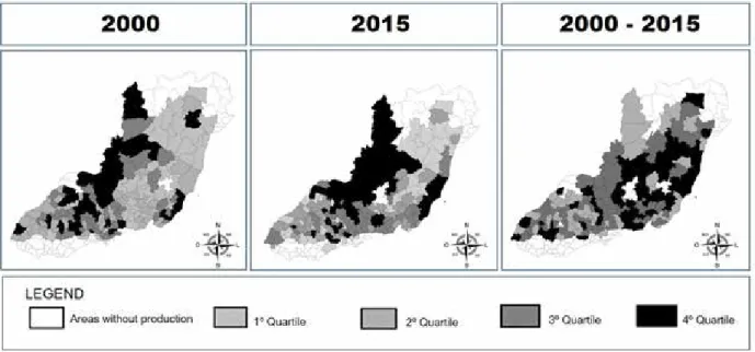
Before the Exploratory Spatial Data Analysis, we attempted to observe the coffee productivity performance in the microregions as well as its growth rate in the 2000 to 2015 period (Figure 3). We can note that in the fourth quartile - the microregions with the highest productivity - are in the western part of Minas Gerais, with only a few regions in the other states. The spatial cof-fee productivity concentration and development is visible in Figure 3, indicating the existence of patterns, which may result in spatial dependence and heterogeneity.
The productivity growth rate between 2000 and 2015, on the other hand, did not show the same pattern as the 2000 and especially 2015
productivities. The growth rate presented a more homogeneous distribution among the microre-gions. However, we can note that many localities with low productivity in both periods presented higher growth rate than microregions with higher initial productivity. For example, the western of Minas Gerais, where the coffee productivity is essentially present in the fourth quartile, are not the region that grew the most during the period considered. This dynamics indicates that we may have a convergence process for coffee produc-tivity between the producing microregions.
It is worth mention that we have some regions in Figure 3 without coffee produc-tion - blank areas on the map - especially the Southern of Paraná and the north of Bahia. One possible explanation is due to the local climatic conditions, since coffee is a crop that fits best in hot and humid climate regions. The Southern Paraná, for example, has a temperate climate, with low temperatures in winter, which makes coffee production unfeasible while in northern Bahia, we have a semi-arid region, also unsuit-able for coffee production.
The Moran’s I captures and reveal the spatial autocorrelation presence in the
georefer-Figure 3. Coffee productivity in the five main producing states.
Source: elaborated with GeoDa (2019).
enced information. We calculated this statistics according to several conventions of spatial matri-ces in order to identify which is the one that better captures the spatial dependence process present in the data. Tables 4 and 5 show the Moran’s I coefficients, its mean, standard deviation, z-value and the p-z-value for the coffee productivity for the years 2000 and 2015, respectively.
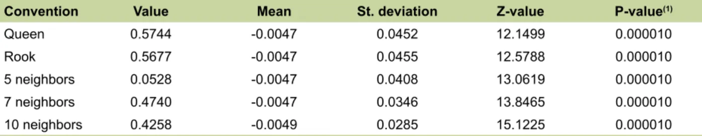
We confirm the spatial dependence existence for both variables and all values are positive, and statistically significant regardless of the convention adopted, indicating that cof-fee productivity tend to be surrounded by mu-nicipalities with similar values. In other words, it indicated that we have spatial autocorrelation for coffee productivity in 2000 and 2015.
The spatial matrix convention that present-ed the largest Moran’ I statistic for both years are the queen matrix. The statistic value for 2000 are 0.5446 whereas for the year 2015 it is 0.5744. Therefore, considering the spatiotemporal evolu-tion, it indicates that the spatial autocorrelation process grew between those years. In addition, we have the Moran’s I statistic, in Table 6, for the growth rate of this variable between the periods (2000-2015).
Table 4. Moran’s I Coefficients for Coffee Productivity – 2000.
Convention Value Mean St. deviation Z-value P-value(1)
Queen 0.5446 -0.0047 0.0453 12.7871 0.000010
Rook 0.5422 -0.0050 0.0456 12.0015 0.000010
5 neighbors 0.0494 -0.0048 0.0410 12.1756 0.000010
7 neighbors 0.4601 -0.0048 0.0344 13.5216 0.000010
10 neighbors 0.3946 -0.0046 0.0285 13.9952 0.000010
(1) Pseudo-empirical significance based on 99999 random permutations.
Table 5. Moran’s I Coefficients for Coffee Productivity – 2015.
Convention Value Mean St. deviation Z-value P-value(1)
Queen 0.5744 -0.0047 0.0452 12.1499 0.000010
Rook 0.5677 -0.0047 0.0455 12.5788 0.000010
5 neighbors 0.0528 -0.0047 0.0408 13.0619 0.000010
7 neighbors 0.4740 -0.0047 0.0346 13.8465 0.000010
10 neighbors 0.4258 -0.0049 0.0285 15.1225 0.000010
(1) Pseudo-empirical significance based on 99999 random permutations.
The local indicator of spatial association (Lisa) is used to provide information on the exis-tence of significant spatial clusters. Figure 4 shows the cluster map for the average productivity of coffee in the microregions during the years 2000, 2015, as well as for the growth rate of the period (2000-2015). The Moran’s I statistics presented positive and significant values for the growth rate variable, which indicates we also have spatial autocorrelation for growth. Therefore, microre-gions that have a high (low) productivity growth are concentrated with regions that also had high (low) growth. The spatial matrix convention that presented the largest Moran’ I statistic for growth
Table 6. Moran’s I coefficient for Coffee productivity growth rate: 2000–2015.
Convention Value Mean St. deviation Z-value P-value(1)
Queen 0.3177 -0.0048 0.0450 7.1555 0.000010
Rook 0.3177 -0.0048 0.0453 7.1272 0.000010
5 neighbors 0.3174 -0.0048 0.0406 7.9770 0.000010
7 neighbors 0.2909 -0.0049 0.0342 8.6476 0.000010
10 neighbors 0.2609 -0.0047 0.0284 9.3537 0.000010
(1) Pseudo-empirical significance based on 99999 random permutations.
are also the queen matrix. However, the value is lower than for those for productivity, which in-dicates that the growth rate has a smaller spatial dependence.
The LISA cluster maps are presented in Figure 4 for the productivities and its growth rate. This statistic have four possible spatial asso-ciation types, i.e., the High-High (HH), Low-Low (LL), High-Low (HL), and Low-High (LH) patterns. In the first map, for the 2000 productivity, we have a HH “corridor” pattern that covers the São Paulo state in the central part, and Minas Gerais in its western part. The second map, related to
2015 productivity, we have a consolidation for the cluster present in the Minas Gerais state, whi-ch, besides maintaining the initial clusters, also expanded to previously non-significant areas, such as the Triângulo Mineiro. On the other hand, it is evident that the São Paulo state loss of relevance regarding its high productivity clusters.
The third cluster map refers to the pro-ductivity growth in the period and its spatial distribution is not the same as for the average productivity. There are two HH clusters for the growth rate, both located in Minas Gerais.
In summary, the coffee productivity beha-vior in the period indicates a consolidation of Minas Gerais as the state with more microregions with high productivity in coffee production. This corroborates Teixeira & Bertella (2015) that argues that coffee productivity in Minas Gerais does not follow a random spatial process. The authors also found a convergence process for this state; however, they do not analyzed the spatial and convergence process considering other relevant states for the Brazilian coffee pro-duction. Therefore, the present paper aims to fill this gap in the literature. The empirical evidences in Table 1, 2, 3 and Figure 2 and 3 corroborates
Figure 4. LISA Map for Coffee Productivity and Growth rate.
Source: elaborated with GeoDa (2019).
that coffee productivity is spatially concentrated in Brazil, especially in the Minas Gerais state. In addition, we seek to analyze if the coffee pro-ductivity is converging in Brazil. The basic hypo-thesis is that the convergence found by Teixeira & Bertella (2015) for Minas Gerais is occurring in a national level.
The OLS and the spatial convergence models are in Table 7. First, we estimate the model with the OLS method in order to verify the existence of spatial dependence in the mo-del residuals, which is performed through tests based on the Lagrange multiplier and the robust Lagrange multiplier. Through these tests, we veri-fied that the SEM model is the most adequate to explain the absolute convergence process of for coffee productivity. Furthermore, the model pre-sented homoscedastic errors, since the Koenker-Basset test had a value of 5.85; in addition, we rejected the heteroscedasticity hypothesis at 1% significance level. Finally, the models errors are normally distributed, since the Jarque-Bera test rejected the null hypothesis of non-normality in the residues with a significance level at 1%. Therefore, we can estimate the models that
incor-porate spatial lag (SAR and SEM) with Maximum Likelihood estimator (Anselin, 1999).
Although the spatial error model (SEM) are the most adequate according the robust Lagrange multiplier, we estimated all the spatial models indi-cated in the methodology in order to check the es-timations robustness. We can note that, in Table 7, all the estimated models presented a significant b coefficient with negative sign, indicating that they managed to capture a convergence process for the coffee productivity in Brazil. The fact that all models presented the same signal for b, and simi-lar coefficients magnitudes, shows robustness for the results found. In summary, the convergence process indicates that the microregions decreased their average productivity differences between 2000 and 2015 period.
Considering the lowest values for the AIC (Akaike) and SC (Schwarz) information criteria, the best model is also the spatial error model (SEM). In addition, the error-lag coefficient (l)
are statistically significant at 5% and assumed a positive value of 0.19. This shows that a micro-region suffers a positive spatial spillover influence from its neighbors, leading to an increase in its productivity. The spatial lag model (SAR), on the other hand, presented a statistically significant coefficient r at 10%, as well as a positive coef-ficient of 0.18, indicating that a microregion can be affected by the coffee productivity growth rate from neighboring locations, although the low significance rate from these variables reflects a weak spatial spillover. Finally, the SLX model did not present statistical significance for its coefficient.
Despite the convergence process confir-mation for coffee productivity, it is not possible to determine directly the magnitude in which it is occurring. For this purpose, we performed a complementary analysis, the speed and half-life of the convergence (equation (7) and (8) in the methodology). The coffee productivity speed (θ)
Table 7. The OLS and Spatial Models Results.
Variable Spatial convergence models
MQO (1) SAR (2) SEM (3) SLX (4)
Constant 0.0262 (0.0255) 0.0274 (0.0251) 0.0282 (0.0273) -0.0166 (0.0319) LOG2000 -0.0289*** (0.0090) 0.02598** (0.0090) -0.0297*** (0.0100) -0.0349** (0.0150) WLOG2000 - - 0.0097 (0.0194) λ - - 0.1900** (0.0947) -ρ - 0.1813* (0.0941) - 0.8400 (0.1400)
Crit. Inf. Akaike -161.734 -163.399 -165.728 -159.988
Crit. Schwarz -155.011 -153.315 -159.005 -149.904 ML ρ (lag) 7.978*** - - -MLR ρ (robust lag) 1.507 - - -ML λ(error) 9.472 *** - - -MLR λ (robust error) 3.001* - - -Nº de obs. 213 213 213 213
Note: the values in parentheses refers to the standard deviation; *** Significant at 1%; ** Significant at 5%. * Significant at 10%; LOG2000 refers to the coffee productivity in 2000.
for the period 2000-2015 presented a value of 0.0017, while the half-life (t) are 407. Hence, the convergence speed - the decrease in the coffee productivity gap between the microregions - is occurring at a rate of approximately 0.17% per year. At this rate, it will take approximately 407 years for them to travel halfway between their respective stationary states. Therefore, despite the presence of a convergence process, this has occurred at a slow pace, and is necessary a con-siderable time to reduce productivity regions’ inequalities, which highlights some concerns, since there are many family farming and regions that depends greatly from coffee production. In the next section, we bring possible consequences from this slow convergence process and feasible solutions, in particular, regarding government agricultural policies.
Discussion
Brazil is currently the largest producer and exporter of coffee in the world. The coffee pro-ductive dynamics, therefore, presented by this crop has significant impacts on the economic and social development of the country, especially in the producing regions. In addition, according to Clemente et al. (2017), in the political decision-making process for regional development, the identification of productivity spatial patterns, and their performance over time are fundamental. Agglomerations and spatial interdependencies is a key factor in stimulating regional develop-ment and generate increasing returns. The facts mentioned are even more necessary and urgent for coffee, given that, according to Mattei (2014), more than a third of this crop are produced by the country comes from family farming, many of them being social and economically vulnerable.
According to Watson & Achinelli (2008) and Carvalho et al. (2016), the liberalization of the international coffee market in the 1990s led to a fall in its price, which has reduced the production profitability, affecting especially the less developed rural areas and small farmers in the Brazil. This scenario had an effect mainly in
the coffee cultivation format; such as land use intensification, which resulted in a productivity fall after a few years due to depletion. The main affected by this dynamic are precisely the most vulnerable farmers, who had no other opportu-nity than coffee growing. In addition, according to Watson & Achinelli (2008), after 1990s, the Brazilian government cut back agricultural sub-sidies and credits, extension services, and rural development initiatives, which served to aggra-vate the small-scale coffee farmer’s situation.
The result found by in this paper can worsen this process, since many regions are not able to increase their productivities, which may possibly amplify the economic and social precariousness of such places. In fact, Krueger (2007), analyzing the social and economic consequences of coffee price fluctuations in the producing regions in Brazil, identified that an important result is an increase in the use of child labor at harvest. According to the author, this measure seeks to increase production and minimize losses, with a consequent decrease in school attendance, especially by vulnerable families. Therefore, the precariousness of the coffee price, combined with the low increase in crop productivity, translated into obstacles for the economic and social development in the producing regions and families.
In addition, the convergence low rate for coffee productivity between the microregions can prolong the negative effects, inhibiting lo-cal development and increasing vulnerability of farmers. Faced with this scenario, several authors have proposed solutions to mitigate the decline in the coffee profitability, especially for regions with low economic and social development. Carvalho et al. (2016), for example, suggests the adoption of more advanced production techniques, as well as measures to intensify the cultivated area use. The result would be the in-crease in the coffee productivity along with its profitability, which would possibly minimize the economic and social problems coming from the fall of its price. However, such attitudes are often impossible without government support, given
the vulnerability and difficulty of poor farmers to invest large sums of money in machinery and technology. In this context, public policies aimed at boosting productivity is essential to offset the economic and social problems. According to Watson & Achinelli (2008), rural credit provision for investment and rural extension are important measures that could be taked by the Brazilian government to help small-scale coffee farmers increase coffee productivity.
Therefore, these policies can act as an in-strument to accelerate the convergence process. Watson & Achinelli (2008) and Ferro-Soto & Mili (2013) emphasizes the importance of the organization of farmers, especially the most vul-nerable, in cooperatives and in the participation of the movement called “Fair Trade”. According to the authors, such movement is a simultaneous combination of social movement and commer-cial collaboration. Its modus operandi is based on the elimination of unnecessary intermediar-ies, the development of brands and certificates for products, codes of conduct for those involved in the production chain, the increase of product quality, as well as its productivity, all under the aegis of producer cooperatives.
According to Ferro-Soto & Mili (2013), Fair Trade has been an efficient form of poor farmers, and regions specialized in coffee growing, to im-prove their social conditions. Despite the higher costs of this type of production, the final price received by producers tends to be higher in certi-fied and higher quality channels, thus increasing their profitability, mitigating the negative effects of the international liberalization of the coffee market. However, Valkila (2014) argues that there are inequalities among Fair Trade-certified farm-ers, with the poorer having lower productivities and production. The raise in final price received by farmers in the Fair Trade benefits more farmer with greater production and productivities.
In fact, Pinto et al. (2014) analyzing so-cioenvironmental certifications in Brazil also identified that the producers that participated in certification are those with higher productivities,
more resources and access to technology. This highlight the fact that most marginalized produc-ers are still unable to access the certification sys-tem and that certification costs could be major constraints to achieving it. The author argues that government policy interventions are necessary to promote new opportunities and productivity improvements among the large numbers of mar-ginalized coffee farmers in Brazil.
Conclusions
The main objective of this paper was to investigate the coffee productivity distribution in Brazil and if it presented a convergence process in the 2000 to 2015 period. As the main contri-bution to the literature, we highlight the spatial dependence and spillovers in the convergence model context, using a Spatial Econometrics approach, in addition to the national geographic cut, since there are no paper in the literature that analyses the spatial patterns and convergence for coffee productivity at national level.
The techniques used indicated a spatial concentration for coffee productivity, a fact that made it necessary to adopt spatial models that incorporated this effect. This spatial concentra-tion can be due to the necessary condiconcentra-tions for cultivating coffee, such as climate, relief, soil and others. Coffee is essentially a tropical crop and requires minimal hydrological conditions to thrive. The microregions that presented high concentration and productivity may be those that best possess the necessary conditions for the coffee culture. However, with the analysis undertaken here, we cannot stated that this is the case, and studies are needed specifically for this issue.
The spatial econometric models (SAR, SEM, SLX), as well as the OLS model, showed a significant and negative sign for the b conver-gence coefficient, evidencing a converconver-gence pro-cess for coffee productivity in the microregions of the five largest producers in Brazil. Among the spatial models, the spatial error model (SEM) presented the best Akaike (AIC) and Schwarz
(SC) information criteria and are the indicated model by the robust Lagrange multiplier, there-fore being the one that explained the most the convergence phenomena of coffee productivity.
Therefore, we have empirical evidences to support convergence process for coffee pro-ductivity in Brazil, which result in reductions in the microregional productivities inequalities between 2000 and 2015. However, according to the convergence speed and half-life comple-mentary analysis, this has taken place slowly, at rate of 0.17% per year, which require a consider-able time to complete the process. Due to the fall in the international price of coffee in the last decades, the slow convergence process may result in low profitability for farmers, especially in less economically developed regions. In addi-tion, socially vulnerable family farmers produce a considerable part of the coffee in Brazil, which aggravates the effects from productivity stagna-tion, especially in regions with lower production per hectare.
To worsen the scenario, Brazilian govern-ment cut back agricultural subsidies and credits, extension services, and rural development initia-tives, which served to aggravate the small-scale coffee farmer’s situation. The slow convergence rate can prolong the negative effects, inhibiting local development and increasing vulnerability of farmers. Some measures to mitigate these effects are highlighted by the literature as, for example, the adoption of more advanced production techniques, as well as measures to intensify the cultivated area use, which could increase coffee productivity along with its profitability. However, such attitudes are difficult without government support, given the vulnerability and difficulty of poor farmers to invest large sums of money in machinery and technology. Therefore, public policies, as rural credit provision for investment and rural extension aimed at boosting produc-tivity is essential to offset the socioeconomic problems, helping small-scale coffee farmers.
In addition, some authors argues farmer’s organization in cooperatives and the participa-tion in the “Fair Trade” movement can induce
the elimination of unnecessary intermediaries, the development of brands and certificates for products, codes of conduct for those involved in the production chain, which would lead to the increase of product quality, as well as its pro-ductivity. Therefore, the policies and measures mentioned can act as an instrument to acceler-ate the convergence process, reducing regional inequalities within the country.
The slow convergence process and the lower profitability resulted with it may not be limited to the coffee crop, extending to other agricultural commodities. Therefore, as future work, we indicate the search for convergence in other cultures in Brazil, or other develop-ing countries with similar economic and social characteristics. We also highlight the search for possible socioeconomic impacts that the slow productivity convergence can have, especially in vulnerable regions and small-scale farmers.
References
ALMEIDA, E. Econometria espacial aplicada. Campinas: Alinea, 2012. 498p.
ALMEIDA, E.S. de; PEROBELLI, F.S. FERREIRA, P.G.C. Existe convergência espacial da produtividade agrícola no Brasil? Revista de Economia e Sociologia Rural, v.46, p.31-52, 2008. DOI: https://doi.org/10.1590/S0103-20032008000100002.
ANSELIN, L. Local indicators of spatial association – LISA. Geographical Analysis, v.27, p.93-115, 1995. DOI: https://doi.org/10.1111/j.1538-4632.1995.tb00338.x. ANSELIN, L. Spatial econometrics. Dallas: University of Texas, 1999.
BAUMOL, W.J. Productivity growth, convergency, and welfare: what the long-run data show. American
Economic Review, v.76, p.1072-1085, 1986.
BRASIL. Secretaria de Política Agrícola. Available at: <www.agricultura.gov.br>. Accessed on: Sept. 20 2017. CARVALHO, A.X.Y. de; LAURETO, C.R.; PENA, M.G.
Agriculture productivity growth in Brazilian micro-regions. Brasília: Ipea, 2016. (Ipea. Discussion paper,
208).
CECAFE. Conselho dos Exportadores de Café do Brasil. Available at: <www.cecafe.com.br>. Acessed on: Sept. 28 2017.
CLEMENTE, A.M.; CARVALHO JÚNIOR, O.B. de; GUIMARÃES, R.F.; MCMANUS, C.; TURAZI, C.M.V.; HERMUCHE, P.M. Spatial-temporal patterns of bean crop in Brazil over the period 1990-2013. International
Journal of Geo-Information, v.6, art.107, 2017. DOI:
https://doi.org/10.3390/ijgi6040107.
CNA. Confederação da Agricultura e Pecuária do Brasil. Available at: <www.cnabrasil.org.br>. Accessed on: Sept. 28 2017.
FERRO-SOTO, C.; MILI, S. Desarrollo rural e
internacionalización mediante redes de Comercio Justo del café. Un estudio del caso. Cuadernos de Desarrollo
Rural, v.10, p.267-289, 2013.
FLORAX, R.J.G.M.; FOLMER, H.; REY, S.J. Specification searches in spatial econometrics: the relevance of Hendry´s methodology. Regional Science & Urban
Economics, v.33, p.557-579, 2003. DOI: https://doi.
org/10.1016/S0166-0462(03)00002-4.
FURTADO, C. Formação Econômica do Brasil. 32.ed. São Paulo: Companhia Editora Nacional, 2003.
GEODA: an introduction to spatial data analysis. Available at: <https://geodacenter.github.io/>. Accessed on: Aug. 12 2019.
IAPAR. Instituto Agronômico do Paraná. Available at: <www.iapar.br>. Accessed on: Oct. 1 2017.
IBGE. Instituto Brasileiro de Geografia e Estatística. Available at: <www.sidra.ibge.gov.br>. Accessed on: Sept. 20 2017.
KELEJIAN, H.H.; PRUCHA, I.R. A generalized moments estimator for the autoregressive parameter in a spatial model. International Economic Review, v.40, p.509-533, 1999. DOI: https://doi.org/10.1111/1468-2354.00027. KRUGER, D.I. Coffee production effects on child labor and schooling in rural Brazil. Journal of Development
Economics, v.82 p.448-463, 2007. DOI: https://doi.
org/10.1016/j.jdeveco.2006.04.003.
LOPES, J.L. Avaliação do processo de convergência
da produtividade da terra na agricultura brasileira no período 1960 a 2001. 2004. 193p. Tese (Doutorado)
- Escola Superior de Agricultura Luiz de Queiroz, Universidade de São Paulo, Piracicaba.
MATTEI, L. O papel e a importância da agricultura familiar no desenvolvimento rural brasileiro
contemporâneo. Revista Econômica do Nordeste, v.45, p.83-91, 2014.
PEROBELLI, F.S.; ALMEIDA, E.S. de; ALVIM, M.I. da S.; FERREIRA, P.G.C. Produtividade do setor agrícola brasileiro (1991-2003): uma análise espacial. Nova
economia, v.17, p.65-91, 2007. DOI: https://doi.
org/10.1590/S0103-63512007000100003.
PINTO, L.F.G.; GARDNER, T.; MCDERMOTT, C.L.; AYUB, O. L. Group certification supports an increase in the diversity of sustainable agriculture network–rainforest alliance certified coffee producers in Brazil. Ecological
Economics, v.107, p.59-64, 2014. DOI: https://doi.
org/10.1016/j.ecolecon.2014.08.006.
QGIS. 2017. Available at: <https://qgis.org/>. Accessed on: Aug. 12 2019.
QUAH, D.T. Regional convergence clusters across Europe. European Economic Review, v.40, p.951-958, 1996. DOI: https://doi.org/10.1016/0014-2921(95)00105-0.
RAIHER, A.P.; OLIVEIRA, R.A. de; CARMO, A.S.S. do; STEGE, A.L. Convergência da produtividade agropecuária do sul do Brasil: uma análise espacial.
Revista de Economia e Sociologia Rural, v.54, p.517-536,
2016. DOI: https://doi.org/10.1590/1234-56781806-94790540307.
REY, S.J.; MONTOURY, B.D. US Regional income convergence: a spatial econometric perspective. Regional
Studies, v.33, p.143-156, 1999. DOI: https://doi.
org/10.1080/00343409950122945.
SOUZA, M.C. de; PEROBELLI, F.S. Análise da distribuição territorial da sojicultura no Brasil: 1991-2003. Revista
Econômica do Nordeste, v.39, p.46-65, 2008.
TEIXEIRA, R.F.A.P.; BERTELLA, M.A. Distribuição espaço-temporal da produtividade média do café em Minas Gerais: 1997-2006. Análise Econômica, ano33, p.275-299, 2015. DOI: https://doi.org/10.22456/2176-5456.25814.
VALKILA, J. Do fair trade pricing policies reduce
inequalities in coffee production and trade? Development
Policy Review, v.32, p.475-493, 2014. DOI: https://doi.
org/10.1111/dpr.12064.
WATSON, K.; ACHINELLI, M.L. Context and contingency: the coffee crisis for conventional small-scale coffee farmers in Brazil. Geographical Journal, v.174, p.223-234, 2008. DOI: https://doi.org/10.1111/j.1475-4959.2008.00277.x.