Acta Scientiarum
http://www.uem.br/acta ISSN printed: 1679-9275 ISSN on-line: 1807-8621
Doi: 10.4025/actasciagron.v40i1.35250 CROP PRODUCTION
Estimating soybean yields with artificial neural networks
Guiliano Rangel Alves1*, Itamar Rosa Teixeira1, Francisco Ramos Melo1, Raniele Tadeu Guimarães Souza1 and Alessandro Guerra Silva2
1
Departamento de Engenharia Agrícola, Universidade Estadual de Goiás, Campus Henrique Santillo, BR-153, Fazenda Barreiro do Meio, 75132-400, Anápolis, Goiás, Brazil. 2
Departamento de Agronomia, Universidade de Rio Verde, Rio Verde, Goiás, Brazil. *Author for correspondence. E-mail: [email protected]
ABSTRACT. The complexity of the statistical models used to estimate the productivity of many crops, including soybeans, restricts the use of this practice, but an alternative is the use of artificial neural networks (ANNs). This study aimed to estimate soybean productivity based on growth habit, sowing density and agronomic characteristics using an ANN multilayer perceptron (MLP). Agronomic data from experiments conducted during the 2013/2014 soybean harvest in Anápolis, Goiás State, B razil, were used to conduct this study after being normalized to an ANN-compatible range. Then, several ANNs were trained to choose the best-performing one. After training the network, a performance analysis was conducted to select the ANN with a performance most appropriate for the problem, and the selected network had a 98% success rate with training data and a 72% data validation accuracy. The application of the MLP to the data used in the experiment shows that it is possible to estimate soybean productivity based on agronomic characteristics, growth habit and population density through AI.
Keywords: Glycine max (L.) Merrill; agronomic characteristics; modeling; MLP; perceptron.
Estimativa da produtividade de soja com redes neurais artificiais
RESUMO. Para estimar a produtividade de muitas culturas, incluído a soja, são utilizados modelos estatísticos complexos, que torna restrito o acesso a essa prática. Uma alternativa a estes modelos é a utilização de sistemas computacionais empregando Redes Neurais Artificiais (RNA). Este trabalho teve por objetivo estimar a produtividade da soja baseada nos hábitos de crescimento, densidade de semeadura e características agronômicas usando RNA do tipo Multilayer Perceptron (MLP). Para isto foram utilizados dados agronômicos da cultura da soja obtidos em experimento conduzido na safra 2013/2014 em Anápolis, Estado de Goiás, Brasil, cujos dados foram normalizados em intervalo compatível para trabalho com RNA e em seguida feito o treinamento de várias RNAs para a escolha da RNA com melhor performance. Após o treinamento das redes, foi realizada a análise de performance para seleção da RNA com a performance mais adequada ao problema. A RNA selecionada apresentou um índice de acerto de 98% com os dados do treinamento e um acerto de 72% com dados de validação. A aplicação das RNAs do tipo MLP nos dados do experimento conduzido demonstram que é possível estimar a produtividade da soja baseando-se nas características agronômicas, hábito de crescimento e densidade populacional por meio da IA.
Palavras-chave:Glycine max (L.) Merrill; características agronômicas; modelagem; MLP; perceptron.
Introduction
Soybeans are currently considered the main agricultural commodity of Brazil, which is the second largest producer of this oilseed. During the 2015/2016 harvest, approximately 95.4 million tons of this grain were produced (Conab, 2017), but there are productivity gaps among regions that are due to several factors during the development of the cultivar in the field. The productivity potential of soybean is genetically determined (Homrich, Wiebke-Strohm, Weber, & Bodanese-Zanettini, 2012), but how this potential can be achieved depends on the effect of limiting factors that act at
different stages during the production cycle (Kron, Souza, & Ribeiro, 2008).
Page 2 of 9 Alves et al.
The use of agronomic traits in soybeans at the R6 stage or later makes it possible to estimate productivity without data from previous stages (Lee & Herbek, 2005). At these later stages, the grains have completely filled the cavity near the pod and are similar to the pods collected at harvest (Oliveira, Silva, Mielezrski, Lima, & Edvan, 2016).
Artificial neural networks (ANNs) are widely applied in research due to their ability to model highly nonlinear systems in which the relationships between variables are unknown or very complex (Russell & Norvig, 2009; Goyal, 2013), and this capability has led to the use of ANNs in different fields of science. In the agricultural sciences, several studies have used ANNs (Zhang, Bai, & Liu, 2007; Alvarez, 2009; Gago, Martínez-Núñez, Landín, & Gallego, 2010; Erzin, Rao, Patel, Gumaste, & Singh, 2010; Soares, Pasqual, Lacerda, Silva, & Donato, 2013; Safa, Samarasinghe, & Nejat, 2015; Alves et al., 2017).
This work aimed to evaluate the possibility of using an artificial neural network as a tool to evaluate the main agronomic traits of soybean cultivars with different growth habits and subjected to different sowing densities to obtain estimates of productivity.
Material and methods
The development of a multilayer perceptron (MLP) artificial neural network (ANN) requires supervised training to adjust the weights of the synapses. Thus, the MLP used in this study to estimate soybean productivity was created using data from an experiment conducted during the 2013/2014 harvest at an experimental site belonging to Emater/Goiás, Anápolis, Goiás State, Brazil (48°18'23'' W, 16°19'44'' S). According to the Köppen classification, the climate is AW humid tropical, that is, characterized by a dry winter and a rainy summer. The soil of the area is classified as a Rhodic Hapludox (dystrophic Red Latosol).
The experiment employed a completely randomized, 3 x 3 factorial design with eight replications. The treatments consisted of three soybean cultivars with different growth habits and types (BRS Valiosa RR, BMX Potencia RR and NA 7337RR) and three plant densities (D1: 245,000 plants ha-1, D2: 350,000 plants ha-1 and D3: 455,000
plants ha-1).
At harvest, the following agronomic characteristics (variables) were evaluated in ten plants from each plot: plant height, number of branches per plant, number of pods per plant,
number of grains per pod, weight of 1,000 seeds (WTS) and grain yield (productivity).
To conduct ANN training, independent variables (cultivars with different growth habits and population density) and dependent variables such as the agronomic characteristics of plant height (PH), number of branches per plant (B), number of pods per plant (P), number of seeds per pod (S), weight of 1,000 seeds (WTS) and grain yield (Prod. kg ha-1)
were selected. These variables were normalized to equalize the ANN input data (Leal, Miguel, Baio, Neves, & Leal, 2015) so that the initial weights of the variables were assumed to be equivalent at the beginning of the training, thus avoiding the difficulties posed by variables with different weights that can prevent the ANN from converging.
In addition to having different magnitudes, variables that are not numerical, such as growth habit variables and population density, should also be considered as categories. It is recommended that the same dummy treatment applied to the variables in multiple regression analysis be followed for these types of variables (Sharma, Sharma, & Kasana, 2007; Bohl, Diesteldorf, Salm, & Wilfling, 2016).
For the other input variables whose values are real numbers, a linear transformation was used. The maximum and minimum values of the variables used in this transformation are shown in Table 1.
Table 1. Values used for Xmin and Xmax by variable.
Variable Unit Xmin Xmax
Plant height (PH) cm 20 200
Number of branches per plant (B) un 1 15
Number of pods per plant (P) un 10 150
Number of seeds per pod (S) un 1 4
Weight of 1,000 seeds (WTS) kg 5 40
Productivity (Prod) kg ha-1 1000 6000
The values used as inputs and the expected results were normalized to values between minus one and one, but after the networks were trained and validated, the resulting value of the network was transformed back to its original quantity. To perform this transformation, Equation 1 was used, considering the minimum and maximum values for each variable (Table 1).
= – – + (1)
where: X = the value of the original quantity, scaledX = the transformed value, Xmax = the
maximum possible value for the variable, Xmin = the
value of the lower limit of the converted value (-1 in this study), and d2 = the value of the upper limit of the converted value (1 in this study).
The input layer was set to begin the development of the multilayer perceptron (MLP). One neuron was used for each of the input variables (Table 2), and the output layer contained one neuron representing productivity. To conduct the training and the validation processes, a program was developed using the Levenberg-Marquardt training algorithm (Schiavo, Prinari, Gronski, & Serio, 2015) and the mean squared error (MSE) performance function, Equation 2, to enable various ANN architecture settings to be explored.
= ∑ = ∑ − ∝ (2)
where: N = the number of data presented for the training, e = the difference between the expected value and the estimated value of the network, t = the value estimated by the network, and α = the expected value.
Table 2. Variables presented to the input neuron layer.
Variable Transformation Description
C2
Category/type Growth habit
C3 D2
Category/type Density D3
PH Linear transformation Plant height
B Linear transformation Number of branches per plant
P Linear transformation Number of pods per plant
S Linear transformation Number of seeds per pod
WTS Linear transformation Weight of 1,000 seeds
C2, C3: Growth habit identification. D2, D3: Density identification.
After designing the program, a training was conducted with 20,000 MLP networks. One thousand networks were trained in each architecture by varying the number of neurons in the hidden layer between one and twenty, following the assumption that 2i+1 neurons in the hidden layer are needed to map any continuous function with i entries.
After completing the neural network training, a file was generated for each training that contained the training data (the parameters used in the training, the content of the training data, and the test, validation and performance sets). Another file was generated containing the consolidated data for all the trainings.
The resulting file contained one line for each trained network (20,000). The columns one to sixty-five were the values estimated by the network, and some columns were added (added columns filled by the formula) (Table 3).
To determine the network with the best performance, some networks were selected using the following criteria: general performance of the experiment, performance of the training set, performance of the validation set, performance of the test set, training R2, validation R2, test R2, and
general R2. Pearson's correlations (training,
validation and tests) followed a decreasing order because the higher the value of the Pearson's correlation, the closer the estimated value to the observed value.
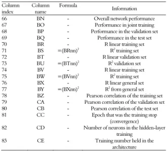
Table 3. Description of the columns in the file containing the information network training data.
Column index
Column name
Formula
Information
66 BN - Overall network performance
67 BO - Performance in joint training
68 BP - Performance in the validation set
69 BQ - Performance in the test set
70 BR - R linear training set
71 BS =(BRnn)2 R2 training set
72 BT - R linear validation set
73 BU =(BTnn)2 R2 validation set
74 BV - R linear training set
75 BW =(BVnn)2 R2 training set
76 BX - R linear general set
77 BY =(BXnn)2 R2 from general set
78 BZ - Pearson correlation of the training set
79 CA - Pearson correlation of the validation set
80 CB - Pearson correlation of the test set
81 CC - Epoch that was the training stop
(convergence)
82 CD - Number of neurons in the hidden-layer
training
83 CE - Training number held in the
architecture
nn: the line number.
Results and discussion
The descriptive statistics of the variables are presented for the test, training and validation of the MLP network (Table 4), and the low number of samples (65 samples) that were used as inputs for the training, validation and testing can be seen. Considering that MLPs learn from examples, this hindered the training and validation of the network.
Page 4 of 9 Alves et al.
Table 4. Descriptive statistics of the variables used to train the ANN.
Characteristic N Average Min Max
Standard
deviation C.V.
Plant height 65 92.37361 78.80 112.18 8.87538 10 %
Branches per
plant 65 4.81704 2.00 11.30 2.09585 44 %
Grains mass per
plant 65 18.18143 10.00 30.57 5.32825 29 %
Nº pods per plant 65 59.63328 27.60 119.80 19.28325 32 %
Seeds per pod 65 2.18204 1.82 2.67 0.27201 12 %
Productivity (kg
ha-1
) 65 4347.56436 2958.72 5248.17 477.41305 11 %
N: number of samples; Min: minimum value; Max: maximum value.
The 65 obtained samples were randomly divided into three subsets: training (42 samples, 65%), validation (16 samples, 25%) and test (7 samples, 10%). For each new training, a new draw was performed, and this division strategy made the training difficult because by performing the random division without considering the treatments used to obtain the samples, the sets were formed with poor sample representation. This resulted in multiple networks with high training performance but a low validation network, with 19 neurons in training 806, line 3, and an observed network performance training with an R2 of 0.999 and
a validation R2 of 0.145 (Table 5).
The development of the program was essential for determining the architecture that could perform adequately because the scaling problem involves the adjusting the complexity of the neural model based on the complexity of the problem. It was possible to vary the complexity of the architecture using the program,
thereby enabling performance evaluation in different architectures and configurations.
Another device was used to repeat the training a thousand times in every architecture. This approach, by which each new training performed a new draw of the training, validation and testing sets, as well as the initialization of the synapse weightings allowed the common problem of tending to get stuck in minimal places when training MLP networks to be overcome using a backpropagation algorithm (Zweiri, Seneviratne, & Althoefer, 2005). The importance of the repetitions was observed in the network with the best performance (R2 = 0.987 in the training and 0.727 in
the validation), which was determined after 963 repetitions in the architecture training with nine neurons in line two of the hidden layers (Table 5).
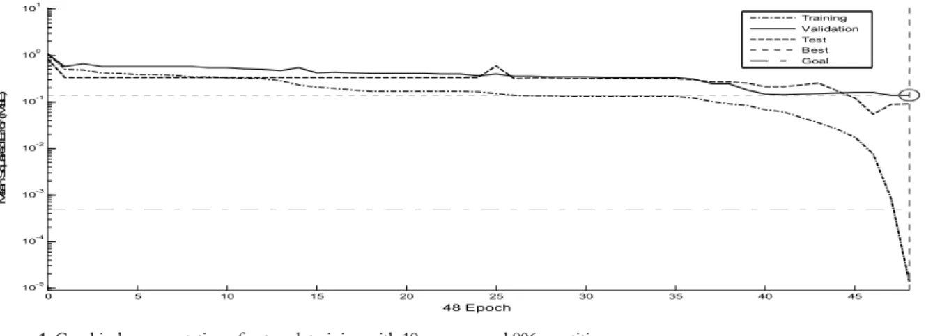
The strategy of drawing new training, validation and test sets during training led to problems regarding the convergence and generalization of the networks because the treatments were not considered. This resulted in the grouping of samples with little representation during the training, test and validation sets and proved that the network began to specialize in the training set. This is illustrated by the high R2 of
0.999 obtained during the network training with 19 neurons after 806 repetitions (Figure 1), at which the training set line near time 48 fell dramatically, indicating that the network had memorized the training set. At the same time, the lines for the validation and test sets did not follow this patterns, showing low R2 values (0.145 and 0.045, respectively).
Table 5. ANN training data.
Training Performance R2 Pearson's correlation
NN NT C Gen Tra Val Test Gen Tra Val Test Gen Tra Val Test
14 124 18 0.009 0.001 0.03 0.03 0.743 0.980 0.240 0.203 0.862 0.990 0.490 0.451
9 963 19 0.03 0.001 0.033 0.155 0.611 0.987 0.727 0.033 0.782 0.993 0.852 0.181
19 806 48 0.044 0.000 0.138 0.092 0.357 0.999 0.145 0.045 0.598 0.999 0.381 0.212
2 212 926 0.028 0.022 0.046 0.021 0.239 0.423 0.000 0.991 0.489 0.650 0.013 0.996
6 336 42 0.029 0.034 0.009 0.048 0.195 0.283 0.264 0.151 0.441 0.532 0.513 0.389
1 340 119 0.033 0.038 0.032 0.003 0.107 0.244 0.041 0.090 0.328 0.494 0.203 0.300
C: cycles or epoch at which the architecture training was finalized; NN: -number of neurons in the hidden layer; NT: training number held in the NN architecture; Tra: training; Val: validation; Performance: mean squared error (MSE) = 7.
Figure 1. Graphical representation of network training with 19 neurons and 806 repetitions.
0 5 10 15 20 25 30 35 40 45
10-5 10-4
10-3 10-2
10-1
100
101
M
ea
n S
q
uar
ed
E
rro
r (
M
S
E
)
48 Epoch
The network with two neurons and 212 repetitions (Figure 2) had the same problem with drawing the sets. The only difference was that the set with the best Pearson's correlation had a value of 99.55 %, but the validation set showed a correlation of only 13.45 %.
Various criteria were used to select the network that best managed to generalize the problem. Networks with fewer neurons in the hidden layer are more generalizable, but a network with few neurons in the hidden layer may not be able to solve a problem with a high degree of complexity and may
result in under fitting (Patterson, 1996). This was observed for the estimated and observed values for the network with a neuron with 340 repetitions (Figure 3) that had an MSE of 0.0315, which was better than the network with nine neurons and 963 repetitions (network chosen as the most appropriate) that presented an MSE of 0.0334. Despite the low MSE, the R2 and the Pearson's correlation values
were not satisfactory (0.041 and -0.203, respectively) (Table 5), and the network failed to model the relationship between the input variables and the expected result.
Figure 2. Graphical representation of network training with 2 neurons and 212 repetitions.
Figure 3. Comparative graphical representation of the estimated and observed values of the validation set for the network with one neuron and 340 repetitions.
0 100 200 300 400 500 600 700 800 900
10-4 10-3 10-2 10-1 100
M
ean Squar
ed
Er
ro
r (
M
SE)
926 Epoch
Training Validation Test Best Goal
2 4 6 8 10 12 14 16
3400 3600 3800 4000 4200 4400 4600 4800 5000 5200
Sample index
G
rai
n y
iel
d (
K
g
)
R2 = 0,041282
Page 6 of 9 Alves et al.
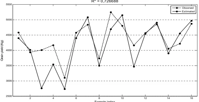
With the validation of the network with nine neurons and 963 repetitions, it was possible to verify the tendency of the observed values to follow the estimated values (Figure 4), which was confirmed by the R2 of 0.726 and the Pearson's
correlation of 85 %. If samples 7 and 11 and indexes 3 and 4 (Figure 4) were removed from this validation, the R2 would rise to 0.811, and the
Pearson's correlation would rise to 90 %. This simulation was performed upon observing that samples 11 and 2 have agronomic characteristics with very similar values but very different productivities (a difference of nearly 800 kg), which raises the possibility that factors that were not recorded in the experiment that created the data influenced the productivity of the samples.
Figure 4. Comparative graphical representation of the estimated and observed values of the validation set for the network with 9 neurons and 963 repetitions.
Among all the trained networks, the one with nine neurons and 963 repetitions, which was selected as the best solution to the problem, did not present the best R2 during training. Rather, it
was selected because it presented the best validation, with an R2 of 0.727 and a Pearson's
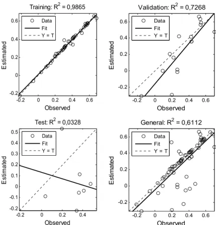
correlation of 85 %. The estimated and observed values were observed to be very close during the training, which is evidence of the learning capacity of the MLP (Figures 5 and 6).
Despite achieving considerable performance during validation (R2 = 0.727 and Pearson’s
correlation = 85%), the selected network had some values that were distant from the line. This can be attributed to the influence of the productivity of the selected samples on the validation set, which was not considered during training. Furthermore, the performance of the test set was very low (R2 =
0.033 and Pearson's correlation = -18%), which reinforces the point that the selection of the sets was entirely random and clustered samples with low representation. The influence of non-registered factors should also be considered.
The difference between the observed and the estimated grain productivity values (error) of the network with the training set was 30.42 kg (Table 6), confirming the high Pearson’s correlation of 99%. The absolute average error was evaluated instead of the average error (17.1 kg) to avoid masking the distance between the observed and estimated values because estimated values may be negative, indicating that the value estimated by the network is greater than the observed, which decreases the average error.
The performance of the MLP was considered good relative to other studies of soybean productivity estimation as represented by Fontana, Berlato, Lauschner, and Mello(2001). This author obtained a correlation of 0.85 between observed and estimated values using the Jensen model modified to estimate the soybean crop yield in the State of Rio Grande do Sul. Using an agrometeorological model, Monteiro and Sentelhas (2014) obtained an R2 of 0.64 when estimating
soybean productivity in different regions.
2 4 6 8 10 12 14 16
2500 3000 3500 4000 4500 5000 5500
Sample index
G
ra
in y
iel
d (
K
g)
R2 = 0,726688
Figure 5. Graphical representation of linear R training, validation, testing and the overall network with 9 neurons and 963 trainings.
Figure 6. Comparative graphical representation of the observed and estimated training values for the network with 9 neurons and 963 repetitions.
Table 6. Analysis of network errors with nine neurons and 963 repetitions.
Samples Min Max Average Mean Absolute Error Deviation
General 65 -841.23 1398.14 122.28 203.78 380.75
Training 42 -216.42 167.81 1.17 30.42 55.85
Validation 16 -351.78 1246.33 193.32 340.56 427.76
Test 7 -841.23 1398.14 686.57 926.92 761.56
Min: minimum; Max: maximum; Mean Absolute Error: average of the absolute error values. Minimum values below zero indicate that the network was estimated above that value. All values are in kg.
-0.2 0 0.2 0.4 0.6
-0.2 0 0.2 0.4 0.6
Observed
Es
ti
m
a
te
d
Training: R2 = 0,9865
Data Fit Y = T
-0.2 0 0.2 0.4
-0.2 -0.1 0 0.1 0.2 0.3 0.4 0.5
Observed
Es
ti
m
a
te
d
Test: R2 = 0,0328
Data Fit Y = T
-0.2 0 0.2 0.4 0.6
-0.2 0 0.2 0.4 0.6
Observed
Es
ti
m
a
te
d
Validation: R2 = 0,7268
Data Fit Y = T
-0.2 0 0.2 0.4 0.6
-0.2 0 0.2 0.4 0.6
Observed
E
s
ti
m
a
te
d
General: R2 = 0,6112
Data Fit Y = T
0 5 10 15 20 25 30 35 40
2500 3000 3500 4000 4500 5000 5500
Sample index
G
rai
n y
iel
d (
K
g)
R2 = 986585
Page 8 of 9 Alves et al.
Conclusion
The multilayer perceptron (MLP) ANN with supervised training could estimate (validation R2 of
0.72 and training R2 of 0.98) a yield with
considerable assertiveness using information regarding the agronomic characteristics, growth habit and population density of the soybean crop.
The use of artificial neural networks to estimate soybean yield is viable, since the back propagation training technique allowed the relationship between the independent variables (soybean agronomic characteristics, growth habit and population density) and soybean yield to be identified with high precision (72%).
References
Akond, A. G. M., Bobby, R., Bazzelle, R., Clark, W., Kantartzi, S. K., Meksem, K., & Kassem, M. A. (2013). Effect to two row spaces on several agronomic traits in soybean [Glycine max (L.) Merr.]. Atlas Journal of Plant Biology,1(2), 18-23. doi: 10.5147/ ajpb.2013.0073 Alvarez, R. (2009). Predicting average regional yield and
production of wheat in the argentine pampas by an artificial neural network approach. European Journal of Agronomy, 30(1), 70-77. doi: 10.1016/ j.eja.2008.07.005 Alves, D. P., Tomaz, R. S., Laurindo, B. S., Laurindo R.
C. F., Fonseca e Silva, F., Cruz, C. D.,... Silva, D. J. H. (2017). Artificial neural network for prediction of the area under the disease progress curve of tomato late blight. Scientia Agricola, 74(1), 51-59. doi: 10.1590/1678-992x-2015-0309
Bohl, M. T., Diesteldorf, J., Salm, C. A., & Wilfling B. (2016). Spot market volatility and futures trading the pitfalls of using a dummy variable approach. The
Journal of Futures Markets, 36(1), 30-45. doi:
10.1002/fut.21723
[Conab] (2017). Companhia Nacional de Abastecimento. Grãos: 4º levantamento da safra 2016/17, janeiro/2017. Brasília, DF: Conab, 2017. Retrieved on Nov. 15, 2017 from: http://www.conab.gov.br/OlalaCMS/uploads/ar quivos/17_01_11_11_30_39_boletim_graos_janeiro_2017 .pdf
Erzin, Y., Rao, B. H., Patel, A., Gumaste, S. D., & Singh, D. N. (2010). Artificial neural network models for predicting electrical resistivity of soils from their thermal resistivity. International Journal of Therm Sciences,49(1), 118-130. doi: 10.1016/ j.ijthermalsci.2009.06.008
Fontana, D. C., Berlato, M. A., Lauschner, M. H., & Mello, R. W. (2001). Modelo de estimativa de rendimento de soja no Estado do Rio Grande do Sul. Pesquisa Agropecuária Brasileira, 36(3), 399-403.
Gago, J., Martínez-Núñez, L., Landín, M., & Gallego, P. P. (2010). Artificial neural networks as an alternative to the traditional statistical methodology in plant research. Journal of Plant Physiology, 167(1), 23-27. doi: 10.1016/j.jplph.2009.07.007
Goyal, S. (2013). Artificial neural networks in vegetables: a comprehensive review. Scientific Journal of Crop Science, 2(7), 75-94. doi: 10.14196/sjcs.v2i7.928
Homrich, M. S., Wiebke-Strohm, B., Weber, R. L. M., & Bodanese-Zanettini, M. H. (2012). Soybean genetic transformation: a valuable tool for the functional study of genes and the production of agronomically improved plants. Genetics and Molecular Biology, 35(4), 998-1010.
Kron, A. P., Souza, G. M., & Ribeiro, R. V. (2008). Water deficiency at different developmental stages of Glycine max can improve drought tolerance. Bragantia, 67(1), 43-49. doi: 10.1590/S0006-87052008000100005 Leal, A. J. F., Miguel, E. P., Baio, F. H. B., Neves, D. C.,
& Leal, U. A. S. (2015). Redes neurais artificiais na predição da produtividade de milho e definição de sítios de manejo diferenciado por meio de atributos do solo. Bragantia, 74(4), 436-444. doi: 10.1590/1678-4499.0140
Lee, C., & Herbek, J. (2005). Estimating soybean yield. Cooperative Extension Service, 188(1), 7-8.
Liu, B, Liu, X. B., Wang, C., Li, Y. S., Jin, J., & Herbert, S. J. (2010). Soybean yield and yield component distribution across the main axis in response to light enrichment and shading under different densities. Plant, Soil and Environment, 56(8), 384–392
Monteiro, L. A., & Sentelhas, P. C. (2014). Calibration and testing of an agrometeorological model for the estimation of soybean yields in different Brazilian regions. Acta Scientiarum. Agronomy, 36(3), 265-272. doi: 10.4025/actasciagron.v36i3.17485
Oliveira, R. D., Silva, C. M., Mielezrski, F., Lima, J. S. B., & Edvan, R. L. (2016). Harvest growth stages in soybean cultivars intended for silage. Acta Scientiarum. Animal Sciences, 38(4), 383-387. doi: 10.4025/actascianimsci. v38i4.31837
Passos, A. M. A., Rezende, P. M., Alvarenga, A. A., Baliza, D. P., Carvalho, E. R., & Alcântara, H. P. (2011). Yield per plant and other characteristics of soybean plants treated with kinetin and potassium nitrate. Ciência e Agrotecnologia, 35(5), 965-972. doi: 10.1590/S1413-70542011000500014
Patterson D. W. (1996). Artificial Neural Networks: Theory and Applications, Simon and Schuster (Asia) Pte. Ltd. Singapore: Prentice Hall
Russell, S., & Norvig, P. (2009). Artificial intelligence: a modern approach. 3. ed. London, UK: Prentice Hall. Safa, M., Samarasinghe, S., & Nejat, M. (2015). Prediction
of wheat production using artificial neural networks and investigating indirect factors affecting it: case study in Canterbury province, New Zealand. Journal of Agricultural Science and Technology, 17(4), 791–803. Schiavo, M. L., Prinari, B., Gronski, J. A., & Serio, A. V.
(2015). An artificial neural network approach for modeling the ward atmosphere in a medical unit. Mathematics and Computers in Simulation, 116(1), 44-58. doi: 10.1016/j.matcom.2015.04.006
Prediction of first lactation 305-day milk yield in karan fries dairy cattle using ann modeling. Applied Soft
Computing, 7(3), 1112-1120. doi:
10.1016/j.asoc.2006.07.002
Soares, J. D. R., Pasqual, M., Lacerda, W. S., Silva, S. O., & Donato, S. L. R. (2013). Utilization of artificial neural networks in the prediction of the bunches’ weight in banana plants. Scientia Horticulturae, 155(1), 24-29. doi: 10.1016/j.scienta.2013.01. 026
Souza, R. T. G.; Teixeira, I. R., Reis, E. F., & Silva, A. G. (2016). Soybean morphophysiology and yield response to seeding systems and plant populations. Chilean
Journal of Agricultural Research, 76(1), 3-8.
doi:http://dx.doi:10.4067/S0718-58392016000100001
Zhang, W., Bai, C., & Liu, G. (2007). Neural network modeling of ecosystems: A case study on cabbage growth system. Ecological Modelling, 201(3-4), 317-325. doi: 10.1016/j.ecolmodel.2006.09.022
Zweiri, Y. H., Seneviratne, L. D., & Althoefer, K. (2005). Stability analysis of a three-term backpropagation algorithm. Neural Networks, 18(10), 1341-1347.
Received on February 6, 2017. Accepted on June 12, 2017.